基於小波混沌分析法之癲癇預測及電路實現

國

立

交

通

大

學

多媒體工程研究所

碩

士

論

文

基於小波混沌分析法之癲癇預測及電路實現

Wavelet-Based Chaos Analysis for Epileptic Seizure Prediction

and Circuit Implementation

研 究 生：王舒愷

指導教授：林進燈 教授

基於小波混沌分析法之癲癇預測及電路實現

Wavelet-Based Chaos Analysis for Epileptic Seizure Prediction and

Circuit Implementation

研 究 生：王舒愷 Student：Shu-Kai Wang

指導教授：林進燈 Advisor：Chin-Teng Lin

國 立 交 通 大 學

多 媒 體 工 程 研 究 所

碩 士 論 文

A Thesis

Submitted to Institute of MultimediaEngineering College of Computer Science

National Chiao Tung University in partial Fulfillment of the Requirements

for the Degree of Master

in

Computer Science January 2009

Hsinchu, Taiwan, Republic of China

中華民國九十八年一月

基於小波混沌分析法之癲癇預測及電路實現

學生：王舒愷

指導教授：林進燈 博士

國立交通大學多媒體工程研究所

中文摘要

在大腦生理訊號分析的研究中，如何從長時間的腦電波訊號找出可靠的特徵 來進行癲癇疾病的預測是目前熱門的研究議題，有鑑於傳統的統計分析方法對於 非穩定、非線性動態系統的訊號，容易因錯誤的結論而影響預測準確性。 本論文提出一個基於小波及混沌理論分析的架構包含離散小波轉換、相關維 度、及相關係數。因小波具有多解析度、時頻分析的特性，相對於傅立葉轉換更 適合用在非穩定訊號。而混沌理論對於非穩定、非線性動態系統的基本推論，比 傳統的統計學方法能更有效地重建腦波的特徵，有助於腦波訊號的分析。因此， 結合小波與混沌理論將可有效提高癲癇預測的準確性及降低誤判率。 本論文提出的作法是先將訊號分解成若干子頻帶，並針對子頻帶，利用腦電 波在癲癇發作前後，其相關維度收歛速度的不同來做為預測的依據。經實驗結 果，本論文所提出的演算法在 11 位具癲癇病患的測試中，可達到 87%的預測準 確率，誤判率為 0.24 次/小時，其平均預測時間約在發病前 27 分鐘。 為了能讓本論文提出的方法能應用於可攜式生理監控設備，我們將其設計成 癲癇分析的處理電路，並針對演算法特性，使用提升式小波轉換、改良記憶體定 址、及其他算數化簡來降低電路面積及功耗，也可於將來進一步整合到生醫的訊 號處理器中。

Wavelet-Based Chaos Analysis for Epileptic

Seizure Prediction and Circuit Implementation

Student：Shu-Kai Wang

Advisor：Dr. Chin-Teng Lin

Institute of Multimedia Engineering, College of Computer Science

National Chiao-Tung University

Abstract

The Epilepsy and epileptic seizure prediction algorithm by extracting useful features from Electroencephalography (EEG) is a hot topic in the current research of physiological signals. In view of the erroneous conclusions from the traditional statistical analysis methods for non-stationary and non-linear dynamics system of signals may affect the accuracy of forecasts.

This thesis presents a novel architecture based on wavelet and chaos theory, including Discrete Wavelet Transform (DWT), correlation dimension, and correlation coefficient. The wavelet transform is more suitable for non-stationary signals than Fast Fourier Transform (FFT) due to the ability of multi-resolution and time- frequency analysis. The fundamentals of Chaos theory for non-stationary and non-linear dynamics systems are more in line with the characteristics of brain waves than statistics. Therefore, combining DWT and Chaos analysis can achieve a high prediction rate.

In this thesis, first EEG signals are decomposed into several subbands. We predict seizures by the difference of convergent radius between the correlation dimension of EEG before a seizure and the one during a seizure for each subband.

The proposed algorithm is evaluated with intracranial EEG recordings from a set of eleven patients with refractory temporal lobe epilepsy. In the experimental results, the algorithm with global settings for all patients predicted 87% of seizures with a false prediction rate of 0.24/h. Seizure warnings occur about 27 min ahead the ictal on average.

To apply the algorithm proposed to a portable physiological monitoring device, a seizure analysis circuit is also designed. Some techniques, such as lifting wavelet transform, enhanced memory addressing, and arithmetic reduction etc., are used to reduce circuit area and power consumption of circuit. In the future, the seizure analysis circuit can be further integrated into a digital signal processor for biomedical applications.

誌謝

本篇論文研究能夠順利完成，要感謝許多人的不管是課業上或精神上的鼓勵 及幫助，讓我在這兩年中獲得專業知識及研究方法。 首先要感謝的就是我的指導教授-林進燈老師。老師在許多領域都有優異的 研究成果，在國內也是頗負盛名，給予我們豐富的學術資源，以及完善的研究環 境，更指導我們面對研究時的態度應該小心謹慎。 另外，也非常感謝帶領指導我們的范倫達教授以及鍾仁峰學長，在畢業方向 的討論上，提供許多重要的意見及建議，在研究過程中，對於學生的疑問或遇到 的問題，總能很有耐心的提供不同面向的觀察，甚至是原本研究忽略掉的細節， 使我面對困難時能有更全面的見解。 也很感謝這段時間在實驗室一起努力的夥伴，智文學長、德瑋學長、紹航學 長、煒忠、儀晟、孟修、寓鈞、孟哲、毓廷、建昇、俊彥以及一群可愛的學弟們， 因為有你們在研究上的扶持與鼓勵，使得我們在實驗室可以一起成長進步。 最感謝的當然還是在背後默默支持我的爸爸、媽媽、爺爺、奶奶、及妹妹， 讓我即使在外求學，因為有你們的關心而感到溫暖，讓我更有信心及勇氣來面對 一切的挑戰。

CONTENTS

中文摘要...i Abstract...ii 誌謝...iv List of Figures...vii List of Tables...ix Chapter 1 Introduction...1

1.1 Epilepsy and Epileptic Seizure ...1

1.2 Motivation...3

1.3 Organization of the Thesis ...4

Chapter 2 Fundamentals of Seizure Analysis Algorithm ...5

2.1 Electroencephalography...5

2.2 Chaotic Modeling for EEG ...7

2.2.1 Introduction to Chaos Theorem ...7

2.2.2 Reconstruction of Attractors from Time Series ...15

2.3 Related Works ...16

Chapter 3 Wavelet-Correlation Dimension Seizure Prediction...21

3.1 Architecture of Seizure Prediction...21

3.2 Discrete Wavelet Transform...23

3.2.1 Discrete Fourier Transform...23

3.2.2 Heisenberg uncertainty principle ...24

3.2.3 Wavelet and Multiresolution Analysis ...25

3.3 Correlation Dimension...39

3.4 Feature Extraction and Prediction Rules...45

Chapter 4 VLSI Implementation and Verification ...50

4.1 Architecture of the Real-Time Seizure Circuit ...50

4.2 Arithmetic Functional Units ...51

4.2.1 Lifting Wavelet ...51

4.2.2 Correlation Dimension...59

4.3 System Controller ...63

4.4 Simulation and Verification ...65

4.5.1 Simulation in Wavelet Circuit...66

4.5.2 Simulation in Correlation Dimension Circuit ...67

Chapter 5 Experimental Results...68

5.1 EEG Data and Patient Characteristics...68

5.2.1 Terminology...69

5.2.2 Seizure Prediction Results ...70

5.3 Comparison with other Prediction Methods ...72

Chapter 6 Conclusions and Future Works ...74

List of Figures

Fig. 1-1 Neurons diagram ...1

Fig. 1-2 Vagus nerve stimulation (VNS)...2

Fig. 2-1 Electrodes positions: contacts in red are chosen from the seizure onset zone and contacts in blue are selected as not involved or involved latest during seizure spread...6

Fig. 2-2 EEG recordings ...6

Fig. 2-3 Time intervals of EEG recordings...6

Fig. 2-4 Logistic map of period-1 cycle...9

Fig. 2-5 Logistic map of period-2 cycle...10

Fig. 2-6 Logistic map of r=3.9...11

Fig. 2-7 Bifurcation diagram for the Logistic map ...12

Fig. 2-8 A plot of Lorenz's strange attractor ...13

Fig. 2-9 Displacement vectors in the fiducial trajectory...17

Fig. 2-10 Unsmoothed STL over time (140 min), including a 2-min seizure. [7]...19

Fig. 2-11 The T-index curves denoting entrainment 55 min before seizure SZ2 [7]. ..20

Fig. 3-1 Typical EEG waveforms corresponding to epilepsy: ...21

Fig. 3-2 System architecture of seizure prediction ...22

Fig. 3-3 A pyramidal image structure and system block diagram for creating it...26

Fig. 3-4 Two image pyramids and their statistics: a approximation (Gaussian) pyramid and a prediction residual (Laplacian) pyramid ...27

Fig. 3-5 (a) A two-band filter bank for one-dimensional subband coding and decoding and (b) its spectrum splitting properties...28

Fig. 3-6 FWT analysis bank...36

Fig. 3-7 Time-frequency tilings for (a) sampled data, (b) FFT, and (c) FWT basis functions...36

Fig. 3-8 (a) Two-level Daubechies 4 wavelet and (b) Time-frequency tilings of EEG37 Fig. 3-9 Analysis and synthesis filters ...38

Fig. 3-10 Decompose the EEG into many subbands ...38

Fig. 3-11 (a) Time blocks, (b) States, and (c) Embedding dimension ...39

Fig. 3-12 Pointwise dimension ...40

Fig. 3-13 Correlation dimension with different radius ...41

Fig. 3-14 Correlation dimension of unfiltered signal...42

Fig. 3-15 Correlation dimension of (a) L1 and (b) LL2 band ...43

Fig. 3-16 Correlation dimension of (a) LH2, and (b) H1 band ...44

Fig. 3-18 Comparison Result of patient 10 between (a) pre-ictal and (b) inter-ictal...45

Fig. 3-19 Correlation coefficients between correlation dimensions in different embedding dimensions...46

Fig. 3-20 The sensitivity with five different correlation coefficients ...47

Fig. 3-21 Prediction results for patient 1 (a) pre-ictal, and (b) inter-ictal...48

Fig. 3-22 Prediction results for patient 7 (a) pre-ictal, and (b) inter-ictal...49

Fig. 4-1 Top level hardware architecture ...50

Fig. 4-2 WCDSP system architecture ...51

Fig. 4-3 Block diagram of predict and update lifting steps...53

Fig. 4-4 Polyphase representation of wavelet transform ...54

Fig. 4-5 Pipelined lifting wavelet architecture of db4 ...55

Fig. 4-6 Multiplier circuit for the coefficient α ...57

Fig. 4-7 Multiplier circuit for the coefficient β ...57

Fig. 4-8 Multiplier circuit for the coefficient γ ...58

Fig. 4-9 Multiplier circuit for the coefficient δ ...58

Fig. 4-10 Multiplier circuit for the coefficient ζ ...59

Fig. 4-11 Correlation dimension circuit...59

Fig. 4-12 Block diagram of correlation dimension...60

Fig. 4-13 Enhanced memory addressing...61

Fig. 4-14 Timing diagram for the original std. formula...62

Fig. 4-15 Timing diagram for the adjusted std. formula ...63

Fig. 4-16 Modified wavelet circuit with two register banks...64

Fig. 4-17 Modified correlation dimension circuit...64

Fig. 4-18 Block diagram of system controller ...65

Fig. 4-19 Wavelet gate-level simulation with two modes...66

Fig. 4-20 Correlation dimension simulation for the first state...67

Fig. 4-21 Correlation dimension simulation results...67

Fig. 5-1 Defining the SPH and SOP ...70

Fig. 5-2 Sensitivity and FPR comparisons with other algorithms ...73

List of Tables

Table 2-1 Results of logistic map (r=2.8) ...9

Table 2-2 Results of logistic map (r=3.14) ...10

Table 2-3 Results of logistic map (r=3.9) ...11

Table 4-1 Two’s complement to CSD conversion...56

Table 4-2 Description of control word...65

Table 5-1 Patient characteristics ...69

Table 5-2 Performance of WCDSP for the optimal setting over all patients ...71

Table 5-3 Comparison with other algorithms ...72

Chapter 1

Introduction

1.1 Epilepsy and Epileptic Seizure

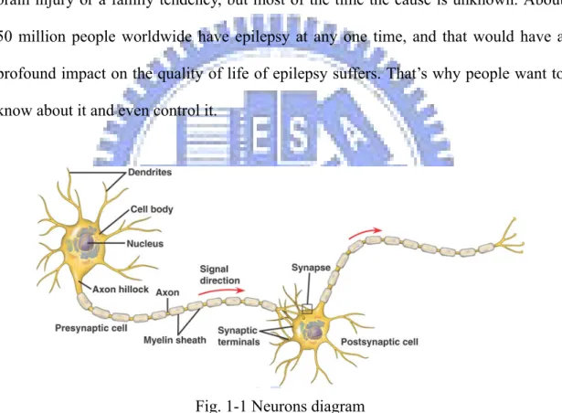
Epilepsy is a common chronic neurological disorder that is characterized by recurrent unprovoked seizures, called Epileptic Seizure (ES). It may be related to a brain injury or a family tendency, but most of the time the cause is unknown. About 50 million people worldwide have epilepsy at any one time, and that would have a profound impact on the quality of life of epilepsy suffers. That’s why people want to know about it and even control it.

Fig. 1-1 Neurons diagram

(From: http://kvhs.nbed.nb.ca/gallant/biology/neuron_structure.html)

These seizures are transient signs or symptoms due to abnormal, excessive or synchronous neuronal activity in the brain. Generally, the brain continuously generates tiny electrical impulses in an orderly pattern. These impulses travel along the network of nerve cells, called neurons, in the brain and throughout the whole body via chemical messengers called neurotransmitters. A seizure occurs when the brain's

nerve cells misfire and generate a sudden, uncontrolled surge of electrical activity in the brain. Epilepsy should not be understood as a single disorder, but rather as a group of syndromes with vastly divergent symptoms but all involving episodic abnormal electrical activity in the brain.

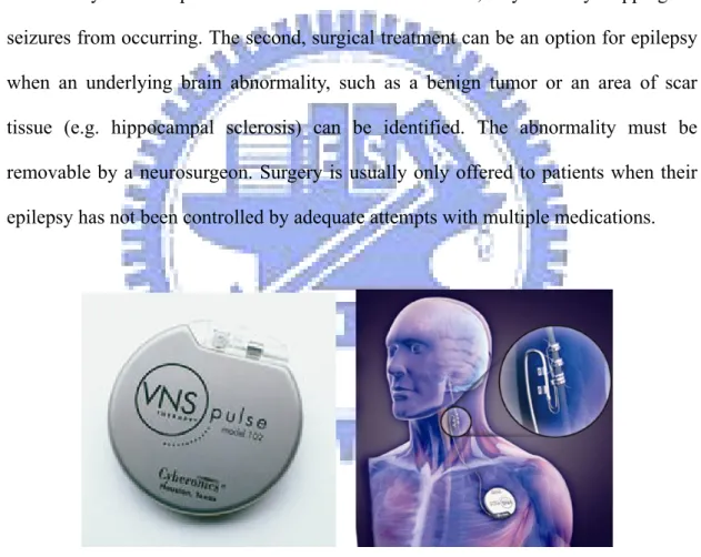
Treatments are available that can successfully prevent seizures for most people with epilepsy. The first treatment is almost always one of the many seizure medicines (also called an antiepileptic drug or AED) that are now available. These medicines do not actually "fix" the problems that cause seizures. Instead, they work by stopping the seizures from occurring. The second, surgical treatment can be an option for epilepsy when an underlying brain abnormality, such as a benign tumor or an area of scar tissue (e.g. hippocampal sclerosis) can be identified. The abnormality must be removable by a neurosurgeon. Surgery is usually only offered to patients when their epilepsy has not been controlled by adequate attempts with multiple medications.

Fig. 1-2 Vagus nerve stimulation (VNS) (From: http://www.medgear.org/page/4/)

Vagus Nerve Stimulation (VNS), shown in Fig. 1-2, is a recently developed form of seizure control which uses an implanted electrical device. It is similar in size, shape and implant location to a heart pacemaker, which connects to the vagus nerve in

the neck. The vagus nerve is part of the autonomic nervous system, which controls functions of the body that are not under voluntary control. Once in place the device can be set to emit electronic pulses, stimulating the vagus nerve at pre-set intervals and milliamp levels. A new research on VNS was a major focus at annual meeting of the American Epilepsy Society in 2000. At a symposium on neurostimulation, it was reported that long-term efficacy studies lasting up to 5 years show that VNS can help a wide array of epilepsy patients who do not respond to seizure medicines and cannot be treated with epilepsy surgery. Overall, the studies indicated that 34% to 48% of these adult patients experienced at least a 50% reduction in seizure frequency after 2 to 5 years of follow-up.

1.2 Motivation

Neurobehavioral disorders can profoundly affect the lives of epilepsy suffers. Thus, identification and treatment of cognitive and behavioral disorders are essential. To enhance the conventional treatments, we think incorporating the VNS or seizure medicines with a seizure prediction algorithm or more accurate to say a seizure precursory analysis algorithm is a feasible solution. Thus, the ability to predict seizures would play an important role to improve the quality of life of the people with epilepsy. In recent years, more and more researches focus on seizure analysis, and a lot of valuable papers are presented, such as Similarity Index [1], Sync decrease [2], Approximate entropy (ApEn) [3] etc. But we can say there is no robust enough algorithm has been published to date.

In view of the erroneous conclusions from the traditional statistical analysis methods for non-stationary and non-linear dynamics system of signals may affect the accuracy of forecasts. To determine the main precursory anomalies from brain waves

more precisely, this thesis presents an architecture based on wavelet and chaos theory, including Discrete Wavelet Transform (DWT), correlation dimension, and correlation coefficient. The wavelet transform is more suitable for non-stationary signals than Fast Fourier Transform (FFT) due to its ability of multi-resolution, and time- frequency analysis. The fundamentals of Chaos Theory for non-stationary and non-linear dynamics systems are more in line with the characteristics of brain waves than statistics. Therefore we can achieve a high prediction rate by combining the DWT and Chaos analysis.

For applying the algorithm proposed into a portable physiological monitoring device, we develop a seizure analysis circuit. Some techniques, such as lifting wavelet transform, an enhanced memory addressing, and arithmetic reduction etc., are used in the design to reduce the area and the power consumption of circuit. In the future, we even can integrate it into a digital signal processor of biomedical applications.

1.3 Organization of the Thesis

This thesis is organized as follows. Chapter 2 introduces the theory of chaos analysis and related works. The proposed algorithm for seizure prediction is described in Chapter 3. Chapter 4 describes the implementation techniques of seizure circuit design. Finally, the experimental results and discussions are presented in Chapter 5.

Chapter 2

Fundamentals of Seizure Analysis

Algorithm

This chapter will introduce the seizure analysis algorithm based on the Chaos Theory. First, we explain what the Electroencephalography (EEG) is, then use the Chaos Theory to model EEG for analysis. After this, two well-known algorithms as short-term Lyapunov exponential and correlation dimension are introduced.

2.1 Electroencephalography

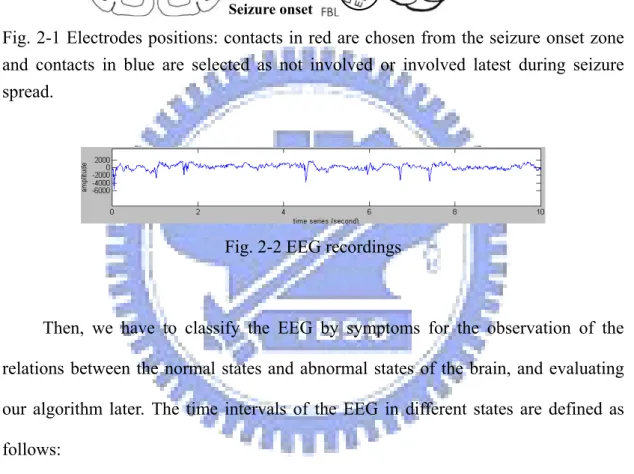
Electroencephalography (EEG) is the measurement of electrical activity produced by the brain as recorded from electrodes. So-called scalp EEG is collected from tens to hundreds of electrodes positioned on different locations at the surface of the head. EEG signals shown in Fig. 2-2 are amplified and digitalized for post processing.

In some situations, such as epileptic studies, when deeper brain activity needs to be recorded with more accuracy than provided by scalp EEG, clinicians use an invasive form of EEG known as intracranial EEG (icEEG) where electrodes are placed directly inside the skull (see Fig. 2-1). In some cases, a grid of electrodes is laid on the external surface of the brain, on dura mater yielding epidural EEG but in other cases, a depth electrode known as subdural EEG (sdEEG) and electrocorticography (ECoG) is placed into brain structures, such as the amygdala or hippocampus. Because of the filtering characteristics of the skull and scalp, icEEG activity has a much higher spatial resolution than surface EEG.

Fig. 2-1 Electrodes positions: contacts in red are chosen from the seizure onset zone and contacts in blue are selected as not involved or involved latest during seizure spread.

Fig. 2-2 EEG recordings

Then, we have to classify the EEG by symptoms for the observation of the relations between the normal states and abnormal states of the brain, and evaluating our algorithm later. The time intervals of the EEG in different states are defined as follows:

(a) Pre-ictal: the period prior to the start of the seizure. (b) Ictal: the seizure onset.

(c) Inter-ictal: the period between seizures. (d) Post-ictal: the period after a seizure.

Fig. 2-3 Time intervals of EEG recordings Seizure onset

2.2 Chaotic Modeling for EEG

Many studies have shown that non-linear analysis could characterize the dynamics of neural network underlying EEG which cannot be obtained with conventional linear approach. In the section, we will explain the properties of non-linear dynamics system and how to build an EEG model for chaotic analysis will be explained in detail.

2.2.1 Introduction to Chaos Theorem

Recall that a Newtonian deterministic system is a system whose present state is fully determined by its initial conditions [4] (at least, in principle), in contrast to a stochastic (or random) system, for which the initial conditions determine the present state only partially, due to noise or other external circumstances beyond our control. For a stochastic system, the present state reflects the past initial conditions plus the particular realization of the noise encountered along the way. So, in view of classical science, we have either deterministic or stochastic systems.

For a long time, scientists avoided the irregular side of nature, such as disorder in a turbulent sea, in the atmosphere, and in the fluctuation of wild–life populations. Later, the study of this unusual results revealed that irregularity, nonlinearity, or chaos was the organizing principle of nature.

A modern scientific term deterministic chaos depicts an irregular and unpredictable time evolution of many (simple) deterministic dynamical systems, characterized by nonlinear coupling of its variables. Given an initial condition, the dynamic equation determines the dynamic process, i.e., every step in the evolution. However, the initial condition, when magnified, reveals a cluster of values within a certain error bound. For a regular dynamic system, processes issuing from the cluster

are bundled together, and the bundle constitutes a predictable process with an error bound similar to that of the initial condition. In a chaotic dynamic system, processes issuing from the cluster diverge from each other exponentially, and after a while the error becomes so large that the dynamic equation losses its predictive power.

For example, in 1960s, Ed Lorenz from MIT created a simple weather model in which small changes in starting conditions led to a marked changes in outcome, called sensitive dependence on initial conditions, or popularly, the butterfly effect (i.e., “the notion that a butterfly stirring the air today in Peking can transform storm systems next month in New York, or, even worse, can cause a hurricane in Texas”). Thus long–range prediction of imprecisely measured systems becomes impossibility.

The character of chaotic dynamics can be illustrated with the logistic map as follows [5] :

1 (1 ) n n n

x ₊ =rx −x , (2.1) a discrete-time analog of the logistic equation for population growth. Here, x_n ≥ is 0

a dimensionless measure of the population in the nth generation, and r≥0 is the

intrinsic growth rate. We restrict the control parameter r to the range 0≤ ≤r 4 so that (2.1) maps the interval 0≤ ≤x 1 into itself.

A. Period-Doubling

Suppose we fix r, choose some initial population x0, and then use (2.1) to

generate the subsequent xn. For the growth rate, we can consider cases as follows.

(1) When r< , the population always goes extinct: 1 x_n → as 0 n→ ∞. (2) When 1< <r 3 the population grows and eventually reaches a non-zero

steady state, called a period-1 cycle.

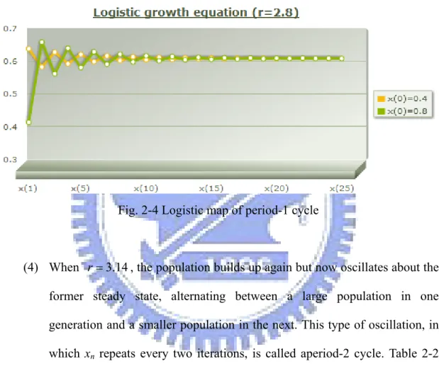
(3) Table 2-1 shows the results of logistic map of initial condition x₀ =0.4 and x₀ =0.8, and we can find that even though there is a huge difference between the initial conditions, the two series as shown in Fig. 2-4 converge

to the same value in a moment.

Table 2-1 Results of logistic map (r=2.8)

Logistic growth equation (r=2.8)

X(0) X(1) X(2) X(3) … X(22) X(23) X(24) X(25)

0.4 0.672 0.617 0.661 … 0.642 0.643 0.642 0.642

0.8 0.448 0.692 0.596 … 0.643 0.642 0.643 0.642

Fig. 2-4 Logistic map of period-1 cycle

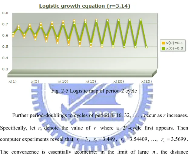
(4) When r=3.14, the population builds up again but now oscillates about the former steady state, alternating between a large population in one generation and a smaller population in the next. This type of oscillation, in which xn repeats every two iterations, is called aperiod-2 cycle. Table 2-2

shows the results of logistic map of initial condition x₀ =0.1 and x₀ =0.3, and the series as shown in Fig. 2-5 reach the same two states after a while.

Table 2-2 Results of logistic map (r=3.14)

Logistic growth equation (r=3.14)

X(0) X(1) X(2) X(3) … X(22) X(23) X(24) X(25)

0.1 0.2826 0.6365 0.7264 … 0.5385 0.7803 0.5382 0.7804

0.3 0.6594 0.7050 0.6527 … 0.7792 0.5402 0.7799 0.5389

Fig. 2-5 Logistic map of period-2 cycle

Further period-doublings to cycles of period 8, 16, 32, . . . , occur as r increases. Specifically, let rn denote the value of r where a 2n-cycle first appears. Then

computer experiments reveal that r₁ = , 3 r₂ =3.449, r₃ =3.54409, …, r_∞ =3.5699. The convergence is essentially geometric: in the limit of large n, the distance between successive transitions shrinks by a constant factor (2.2).

1 1 lim n n 4.669 n n n r r r r δ − →∞ + − = = − (2.2)

In fact, the same convergence rate appears no matter what unimodal map is iterated. In this sense, the number δ is universal. It is a new mathematical constant, as basic to period-doubling as n is to circles.

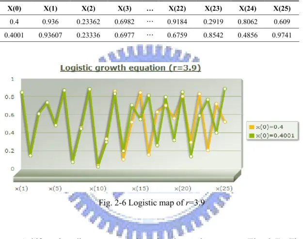
When r r> , the answer turns out to be complicated: For many values of r , _∞ the sequence

{ }

x_n never settles down to a fined point or a periodic orbit instead the

long-term behavior is aperiodic. Table 2-3 shows the results of logistic map. It is interesting to note that even though the difference of the initial conditions is only 0.0001, the two series as shown in Fig. 2-6 are totally divergent in a minute.

Table 2-3 Results of logistic map (r=3.9)

Logistic growth equation (r=3.9)

X(0) X(1) X(2) X(3) … X(22) X(23) X(24) X(25)

0.4 0.936 0.23362 0.6982 … 0.9184 0.2919 0.8062 0.609

0.4001 0.93607 0.23336 0.6977 … 0.6759 0.8542 0.4856 0.9741

Fig. 2-6 Logistic map of r=3.9

A bifurcation diagram summarizes the above phenomenon (Fig. 2-7). The horizontal axis shows the values of the parameter r while the vertical axis shows the possible values of x.

At r=3.4, the attractor is a period-2 cycle, as indicated by the two branches. As r increases, both branches split simultaneously, yielding a period-4 cycle. This splitting is the period-doubling bifurcation mentioned earlier. A cascade of further period-doublings occurs as r increases, yielding period-8, period-16, and so on, until at r r= _∞ ≈3.57, the map becomes chaotic and the attractor changes from a

finite to an infinite set of points.

Fig. 2-7 Bifurcation diagram for the Logistic map

B. Basic Terms of Nonlinear Dynamics

Recall that nonlinear dynamics is a language to talk about dynamical systems. Here, brief definitions are given for the basic terms of this language [4].

z Dynamical system: A part of the world which can be seen as a self–contained entity with some temporal behavior. Mathematically, a dynamical system is defined by its state and by its dynamics.

z Phase space: In mathematics and physics, a phase space, introduced by Willard Gibbs in 1901, is a space in which all possible states of a system are represented, with each possible state of the system corresponding to one unique point in the phase space.

z Attractor: An attractor is a ‘magnetic set’ in the system’s phase space to which all neighboring trajectories converge. More precisely, we define an attractor to be a subset of the phase space with the following properties:

(1) It is an invariant set;

(2) It attracts all trajectories that start sufficiently close to it; (3) It is minimal (it cannot contain one or more smaller attractors).

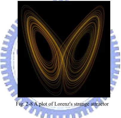
A strange attractor shown in Fig. 2-8 is defined to be an attractor that exhibits sensitive dependence on initial conditions. Geometrically, an attractor can be a point, a curve, a manifold, or even a complicated set with a fractal structure known as a strange attractor.

Fig. 2-8 A plot of Lorenz's strange attractor

z Fractal: Roughly speaking, fractals are complex geometric shapes with fine structure at arbitrarily small scales. Usually they have some degree of self-similarity. In other words, if we magnify a tiny part of a fractal, we will see features reminiscent of the whole. Sometimes the similarity is exact; more often it is only approximate or statistical.

Fractals are of great interest because of their exquisite combination of beauty, complexity, and endless structure. They are reminiscent of natural objects like mountains, clouds, coastlines, blood vessel networks, and even broccoli, in a

way that classical shapes like cones and squares can't match.

z Embedding dimension: The number of variables needed to characterize the state of the system. Equivalently, this number is the dimension of the phase space.

z Fractal dimension: The strange attractors typically have fractal microstructure. The attractor dimension counts the effective number of degrees of freedom in the dynamical system, described by a non integer dimension.

C.

The link between EEG and chaos

Within the context of brain dynamics [4], there are suggestions that “the controlled chaos of the brain is more than an accidental by–product of the brain complexity” and that “it may be the chief property that makes the brain different from an artificial intelligence machine”. Namely, Chaos drives the human brain away from the stable equilibrium, thereby preventing the periodic behavior of neuronal population bursting.

The EEG, being the output of a multidimensional system [6], has statistical properties that depend on both time and space. Components of the brain (neurons) are densely interconnected and the EEG recorded from one site is inherently related to the activity at other sites. This makes the EEG a multivariable time series. The analysis of such nonlinear dynamical systems from time series involves state space reconstruction, and we will introduce in the next section.

If prediction becomes impossible, it is evident that a chaotic system can resemble a stochastic system, say a Brownian motion. However, the source of the irregularity is quite different. For chaos, the irregularity is part of the intrinsic dynamics of the system, not random external influences. Usually, though, chaotic

systems are predictable in the short–term. This short–term predictability is useful. Chaos theory has developed special mathematical procedures to understand irregularity and unpredictability of low–dimensional nonlinear systems. Lyapunov exponents and attractor dimension are some examples. Lyapunov exponents evaluate the sensitive dependence to initial conditions estimating the exponential divergence of nearby orbits, and we will discuss the method later. Correlation dimensions estimate the fractal dimension and will be described in Chapter 3.

2.2.2 Reconstruction of Attractors from Time Series

Roux et al. (in 1983) exploited a surprising data-analysis technique, now known as attractor reconstruction (Packard et al. 1980, Takens 1981). The claim is that for systems governed by an attractor, the dynamics in the full phase space can be reconstructed from measurements of just a single time series.

Construction of the embedding phase space from a data segment ( )x t of duration T is made with the method of delays [6]. The vectors X in the phase space _i

are constructed as

( ( ), ( ) ( ( 1) ))T

i i i i

X = x t x t +τ …x t + p− τ , (2.3)

where τ is the selected time delay between the components of each vector in the phase space, p is the selected dimension of the embedding phase space, and

i

t ∈[1,T -(p - 1)τ]. Obviously, the accuracy of computation depends on the sampling step Δt which decides the number of vectors N_a within a duration T data

segment:

( )

0 1 i

t = + −t i * tΔ , where i∈

[

1,N_a

]

, (2.4) where t₀ is the initial time point of the fiducial trajectory and coincides with the time

The embedding dimension p can be determined from (2.5) if the attractor dimension d is known.

2 1

p≥ d+ (2.5) The choice of delay τ may also significantly affect the metric characteristics

of an attractor. If τ is too small, the ith and the (i+1)th coordinates of a phase point are practically equal to each other. In this case, the reconstructed attractor is situated near the main diagonal of the embedding space, the latter complicating its diagnostics. When a value for τ is chosen that is too large, the coordinates become uncorrelated, and the structure of reconstructed attractor is lost.

2.3 Related Works

A chaotic attractor is an attractor where, on the average, orbits originating from similar initial conditions (nearby points in the phase space) diverge exponentially fast (expansion process); they stay close together only for a short time. If these orbits belong to an attractor of finite size, they will fold back into it as time evolves (folding process). The Lyapunov exponents measure the average rate of expansion and folding that occurs along the local eigen-directions within an attractor in phase space. For an attractor to be chaotic, the largest Lyapunov exponent (LLE) must be positive.

As we mentioned before, a relevant time scale should always be used in order to quantify the physiological changes occurring in the brain. Furthermore, the brain being a nonstationary system, algorithms used to estimate measures of the brain dynamics should be capable of automatically identifying and appropriately weighing existing transients in the data.

Iasemidis et al. developed a method [7] for estimation of short-term Lyapunov exponents (STL), an estimate of LLE for nonstationary data. It is well-known and

widely used in many researches. Here we will take an epileptic seizure prediction system, proposed by L. D. Iasemidis et al. in the recent years, for example to explain the STL in detail.

The short-term Lyapunov exponent (STL) is defined as:

, 2 1 , ( ) 1 log (0) a N i j i a i j X t L N t X δ δ = Δ = Δ

∑

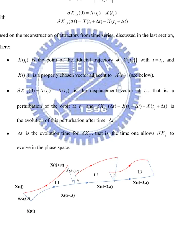
(2.6) with , , (0) ( ) ( ) ( ) ( ) ( ) i j i j i j i j X X t X t X t X t t X t t δ δ = − Δ = + Δ − + Δ

based on the reconstruction of attractors from time series, discussed in the last section, where:

z X t( )_i is the point of the fiducial trajectory φ_t

(

X t

( )

₀

)

with t t= , and _i ( )_j

X t is a properly chosen vector adjacent to X t( )_i (see below).

z δX_{i j,} (0)=X t( ) ( )_i − X t_j is the displacement vector at t_i , that is, a perturbation of the orbit at t_i, and δX_{i j,} ( )Δ =t X t(_i + Δ −t) X t( _j + Δ is t) the evolution of this perturbation after time Δt.

z Δt is the evolution time for δX_ij, that is, the time one allows δX_ij to evolve in the phase space.

Fig. 2-9 Displacement vectors in the fiducial trajectory

L1 L2 L3 X(ti) X(tj) X(tj+Δt) X(ti+Δt) δXij(0) δXij(Δt) θ θ X(ti+2Δt) X(ti+3Δt)

The crucial parameter is the adaptive estimation in time and phase space of the magnitude bounds of the candidate displacement vector to avoid catastrophic replacements. The improvement in the estimates of L can be achieved by using the proposed modifications.

z For L to be a reliable estimate of STL, the candidate vector ( )X t_j should be chosen such that the previously evolved displacement vector

( 1),i j( )

X t

δ ₋ Δ is almost parallel to the candidate displacement vector

, (0) i j X δ , that is, , (0), 1, ( ) max ij i j i j V = δX δX ₋ Δt ≤V (2.7) where V_max should be small and ε φ, denotes the absolute value of the

angular separation between two vectors.

z For L to be a reliable estimate of STL, δX_{i j,} (0) should also be small in magnitude in order to avoid computer overflow in the future evolution within very chaotic regions and to reduce the probability of starting up with points on separatrices. This means,

, (0) ( ) ( ) max i j i j

X X t X t

δ = − < Δ (2.8) with Δ_max assuming small values.

A typical long-term plot of STL versus time, obtained by analysis of continuous EEG, is shown in Fig. 2-10. This figure shows the evolution of STL at a focal electrode site, as the brain progresses from interictal to ictal to postictal states. There is a gradual drop in STL over approximately 2 hours preceding this seizure. The seizure, 2 minutes in duration, is characterized by a sudden drop in STL values with a

consequent steep rise. Postictal STL values exceed preictal values and slowly approach interictal values. This behavior of STL indicates a gradual preictal reduction in chaoticity, reaching a minimum shortly after seizure onset, and a postictal rise in chaoticity that corresponds to the reversal of the preictal pathological state. There will be more discussions about this character in Chapter 3.

Fig. 2-10 Unsmoothed STL over time (140 min), including a 2-min seizure. [7]

Having estimated the STL temporal profiles at each electrode site, and as the brain proceeds toward the ictal state, the temporal evolution of the stability of each cortical site is quantified. However, since the brain is a system of spatial extent, information about the interactions of its spatial components should also be taken in consideration by the relations of the STL between different cortical sites.

The T- index at time t between electrode sites i and j is then defined as:

( )

( )

{

}

i , j

( )

i , j i j t T E STL t STL t N σ = − ÷ , (2.9) where E

{ }

denotes the average of all absolute differences STL t_i

( )

−STL t_j

( )

within a moving window w_t

( )

λ defined as:

( )

1 t

w λ = for λ∈[t-N-1,t] and w

( )

λ =0 for λ∉[t-N-1,t]

where N is the length of the moving window. Then, σ_{i , j}

( )

t is the sample standard deviation of the STL differences between electrode sites i and j within the moving window.

A dynamical transition toward a seizure is announced at time _{t when the} *

T-indexes of sites over time transits from a value above threshold T1 at times t t'< , to a value below threshold T2 at time t , as shown in Fig. 2-11. *

Fig. 2-11 The T-index curves denoting entrainment 55 min before seizure SZ2 [7].

The method presented achieved amazing results with high prediction sensitivity, and pretty low false prediction rate. More details and comparison results with other algorithms and ours will be listed in Chapter 5.

Chapter 3

Wavelet-Correlation Dimension

Seizure Prediction

In this chapter a real-time seizure prediction method based on correlation dimension analysis is presented, including the system architecture, data flow, and algorithms.

3.1 Architecture of Seizure Prediction

Before starting the prediction processing, first we observe the EEG signal whether exists any clue around the seizures. For example, as show in Fig. 3-1, for different clinical states including pre-ictal, ictal, and post-ictal states, the corresponding properties of intracranial EEG recordings are different.

Fig. 3-1 Typical EEG waveforms corresponding to epilepsy: (a) pre-ictal, (b) ictal, and (c) post-ictal

In the pre-ictal state the EEG signal is of the chaotic nature. As we approach the epileptic seizure the signals are less and less chaotic and take the regular shape. These findings imply that seizures may represent spatiotemporal transitions of the epileptic brain from chaos-to-order-to-chaos. Therefore the chaoticity measure of the signal is a good prognostic of the incoming seizure. In fact, this phenomenon is confirmed by STL in the last chapter, but we try to use another method to prove it.

In this chapter, we would propose a Wavelet-Correlation Dimension based Seizure Prediction system, called WCDSP, as shown in Fig. 3-2. The system is consisted of three primary parts:

z Discrete Wavelet Transform analysis: Wavelet is used to decompose the EEG into several sub-bands.

z Chaos analysis: Correlation dimension is used to measure the EEG complexity. z Feature extraction: The correlation coefficient is used to be the main feature for

prediction rules and to decide the seizure states.

Phase Space Reconstruction

Correlation Coefficient

Prediction Rules

3.2 Discrete Wavelet Transform

We would introduce the discrete wavelet transform (DWT) in this section, and briefly discuss the properties of the discrete Fourier transform (DFT), the short-time Fourier transform (STFT), and the wavelet transform.

3.2.1 Discrete Fourier Transform

In mathematics, the discrete Fourier transform (DFT) is one of the specific forms of Fourier analysis, and is widely employed in signal processing and related fields to analyze the frequencies contained in a sampled signal. As such, it transforms one function into another, which is called the frequency domain representation of the original function (which is often a function in the time domain).

The sequence of N complex numbers x ,...,x_{0 N−1} is transformed into the sequence of N complex numbers X ,..., X_{0 N−1} by the DFT according to the formula

( )

1 2 0 i N _kn N n n ˆf X k x e π − ₋ = = =

∑

, k=0,...,N− 1 (3.1) The importance of the Fourier transform stems not only from the significance of

their physical interpretations, such as time-frequency analysis of signals, but also from the fact that Fourier analytic techniques are extremely powerful.

While Fourier analysis forces us to choose between time on one side of the transform and frequency on the other, “…our everyday experiences insist on a description in terms of both time and frequency,” Gabor wrote. To analyze a signal in both time and frequency, he used the windowed Fourier transform. The idea is to study the frequencies of a signal segment by segment; the way, one can at least limit the span of time during witch something is happening. The “window” that defines the size of the segment to analyzed — and which remains fixed in size — is a little piece of curve.

One of the downfalls of the STFT is that it has a fixed resolution. The width of the windowing function relates to the how the signal is represented — it determines whether there is good frequency resolution (frequency components close together can be separated) or good time resolution (the time at which frequencies change).

3.2.2 Heisenberg uncertainty principle

We want to construct a function f whose energy is well localized in time and whose Fourier transform ˆf has an energy concentrated in a small frequency neighborhood.

The Heisenberg principle [8] says the following. For every function f t

( )

, such that

( )

2 1 f t dt ∞ −∞ =

∫

(3.2)

The product of the variance of t and the variance of τ (the variable of ˆf ) is at least ₂

16

h

π , where h is the Planck's constant:

(

) ( )

(

2 2

)

(

(

) ( )

2 2

)

2 16 m m variance of t variance of h ˆ t t f t dt f t d τ τ τ τ π ∞ ∞ −∞ − −∞ − ≥

∫

∫

(3.3)

These variances measure to what extent t and τ take values far from their average values, t and _m τ_m. Thus the shorter-lived a function, the wider the band of frequencies given by its Fourier transform; the narrower the band of frequencies of its Fourier transform, the more the function is spread out in time. Time and frequency energy concentrations are restricted by the Heisenberg uncertainty principle.

3.2.3 Wavelet and Multiresolution Analysis

Unlike the Fourier transform, whose basis functions are sinusoids, wavelet transforms are based on small waves, called wavelets [9], of varying frequency and limited duration. This allows them to provide the equivalent of a musical score for a signal, revealing not only what notes (or frequencies) to play but also when to play them. Conventional Fourier transforms, on the other hand, provide only the notes or frequency information; temporal information is lost in the transformation process.

In 1987, wavelets were first shown to be the foundation of a powerful new approach by Mallat to signal processing and analysis called multiresolution theory. Multiresolution theory incorporates and unifies techniques from a variety of disciplines, including subband coding from signal processing, quadrature mirror filtering from digital speech recognition, and pyramidal image processing. As its name implies, multiresolution theory is concerned with the representation and analysis of signals at more than one resolution. The appeal of such an approach is obvious—features that might go undetected at one resolution may be easy to spot at another.

A. Background

When we look at images, generally we see connected regions of similar texture and gray level that combine to form objects. If the objects are small in size or low in contrast, we normally examine them at high resolutions; if they are large in size or high in contrast, a coarse view is all that is required. If both small and large objects—or low and high contrast objects—are present simultaneously, it can be advantageous to study them at several resolutions. This, of course, is the fundamental motivation for multiresolution processing.

(1) Image Pyramids

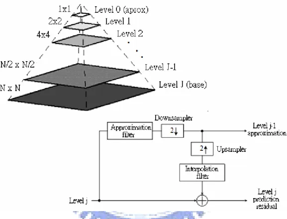
An image pyramid is a collection of decreasing resolution images arranged in the shape of a pyramid. As can be seen in Fig. 3-3, the base of the pyramid contains a high-resolution representation of the image being processed; the apex contains a low-resolution approximation. As you move up the pyramid, both size and resolution decrease.

Fig. 3-3 A pyramidal image structure and system block diagram for creating it

The level j− approximation output is used to create approximation pyramids, 1 which contain one or more approximations of the original image. The level j prediction residual output is used to build prediction residual pyramids.

For example, Fig. 3-4 shows one possible approximation (Gaussian) and prediction residual (Laplacian) pyramid for the vase. The Laplacian pyramid contains the prediction residuals needed to compute its Gaussian counterpart. To build the Gaussian pyramid, we begin with the Laplacian pyramid's level j 64 by 64

approximation image, predict the Gaussian pyramid's level j+ 128 by 128 1 resolution approximation (by upsampling and filtering), and add the Laplacian's level

1

j+ prediction residual. This process is repeated using successively computed approximation images until the original 512 by 512 image is generated.

Fig. 3-4 Two image pyramids and their statistics: a approximation (Gaussian) pyramid and a prediction residual (Laplacian) pyramid

(2) Subband Coding

Another important imaging technique with ties to multiresolution analysis (MRA) is subband coding. In subband coding, an image is decomposed into a set of band-limited components, called subbands, which can be reassembled to reconstruct the original image without error. Since the bandwidth of the resulting subbands is smaller than that of the original signal, the subbands can be downsampled without loss of information. Reconstruction of the original signal is accomplished by upsampling, filtering, and summing the individual subbands.

decoding system. The input of the system is a one-dimensional, band-limited discrete-time signal x n

( )

for n=0 1 2, , ,...; the output sequence, ˆx n

( )

, is formed through the decomposition of x n

( )

into y n₀

( )

and y n₁

( )

via analysis filters

( )

0

h n and h n₁

( )

, and subsequent recombination via synthesis filters g n₀

( )

and

( )

1

g n . Note that filters h n₀

( )

and h n₁

( )

are half-band digital filters whose idealized transfer characteristics, H and ₀ H , are shown in Fig. 3-5(b). ₁

( )

ˆx n

( )

x n ( ) 0 y n ( ) 1 y n (a) (b)

Fig. 3-5 (a) A two-band filter bank for one-dimensional subband coding and decoding and (b) its spectrum splitting properties

Filter H is a low-pass filter whose output is an approximation of ₀ x n

( )

; filter

1

H is a high-pass filter whose output is the high frequency or detail part of x n

( )

. We wish to select h n₀

( )

, h n₁

( )

, g n₀

( )

, and g n₁

( )

so that the input can be reconstructed perfectly. That is, so that ˆx n

( ) ( )

=x n .

We can express the system's output as:

( )

( ) ( )

( ) ( ) ( )

( ) ( )

( ) ( ) ( )

0 0 1 1 0 0 1 1 1 2 1 2 ˆX z H z G z H z G z X z H z G z H z G z X z ⎡ ⎤ = _⎣ + _⎦ ⎡ ⎤ + _⎣ − + − _⎦ − (3.4)

For error reconstruction of the input, ˆx n

( ) ( )

=x n and ˆX z

( )

=X z

( )

. Thus, we impose the following conditions:

( ) ( )

( ) ( )

( ) ( )

( ) ( )

0 0 1 1 0 0 1 1 2 0 H z G z H z G z H z G z H z G z + = − + − = (3.5)

Both can be incorporated into the single matrix expression

( )

( )

( )

[

]

0 1 m 2 0

G z G z H z

⎡ ⎤ =

⎣ ⎦ (3.6)

where analysis modulation matrix H_m

( )

z is

( )

0

_{( )}

( )

0

_{( )}

( )

1 1 m H z H z H z H z H z ⎡ − ⎤ = ⎢ ₋ ⎥ ⎣ ⎦ (3.7)

Assume H_m

( )

z is nonsingular, we can transpose (3.6) and left multiply by inverse

( )

(

_T

)

1 m H z − to get

( )

( )

(

( )

)

( )

( )

0 1 1 0 2 m G z H z G z det H z H z ⎡ ⎤ ⎡ − ⎤ = ⎢ ⎥ ⎢_{− −} ⎥ ⎣ ⎦ ⎣ ⎦ (3.8) For FIR filters, the determinate of the modulation matrix is a pure delay.

( )

(

)

(2k 1)

m

det H z = ⋅α z− +

Ignoring the delay and let α =2

[ ]

( )

[ ]

[ ]

( )

[ ]

0 1 1 1 0 1 1 n n g n h n g n + h n = − = − Define

( )

( ) ( )

( )

(

)

( ) ( )

0 0 0 1 2 m P z G z H z H z H z det H z = = −

Then,

( ) ( )

( )

(

)

( ) ( )

( )

1 1 0 1 2 m G z H z H z H z P z det H z − = − = −

( ) ( )

( ) ( )

[ ] [

]

( )

[ ] [

]

[ ]

[ ] [

]

[ ] [

]

[ ]

0 0 0 0 0 0 0 0 0 0 0 0 2 1 2 2 2 n k k k H z G z H z G z g k h n k g k h n k n g k h n k g k ,h n k n δ δ ⇒ + − − = ⇒ − + − − = ⇒ − =< − >=

∑

∑

∑

Similarly, we can show that

[ ] [

]

[ ]

[ ] [

]

[ ] [

]

1 1 0 1 1 0 2 2 0 2 0 g k ,h n k n g k ,h n k g k ,h n k δ < − >= < − >= < − >= That is,

[

2

] [ ]

[

] [ ]

i j h n k ,g k δ i j δ n < − >= − i, j=

{ }

0 1, (3.9) Filter banks satisfying this condition are called biorthogonal. Moreover, the analysis

and synthesis filter impulse responses of all two-band, real-coefficient, perfect reconstruction filter banks are subject to the biorthogonality constraint.

Orthonormal filter banks:

[

] [ ]

[

] [ ]

{ }

[ ] [

]

[

] [ ]

{ }

2 0 1 2 0 1 i j i i h n k ,g k i j n i, j , g k ,g n m i j m i, j , δ δ δ δ < − >= − = < + >= − = (3.10)

[ ]

( )

[

]

[ ]

[

]

{ }

1 1 0 2 1 2 1 0 1 n i i g n g k n h n g k n , i , = − − − = − − = (3.11)

B. Multiresolution Expansions

In MRA, a scaling function is used to create a series of approximations of a function, each differing by a factor of 2 from its nearest neighboring approximations. Additional functions, called wavelets, are then used to encode the difference in information between adjacent approximations.

A function f x

( )

can be decomposed into a linear combination of expansion functions as follows.

( )

k k

( )

k

f x =

∑

α ϕ x

If the expansion is unique, the ϕ_k

( )

x are called basis functions. The expressible function forms a function space

{

_k

( )

}

k

V =span ϕ x .

For any function space V and corresponding expansion set

{

ϕ_k

( )

x

}

, there exist a set of dual functions, denoted

{

ϕ_k

( )

x

}

, which can be used to compute the α_k coefficients for any f x

( )

∈V.

( ) ( )

*

( ) ( )

k x , f xk x f x dxk

α = <ϕ > =

∫

ϕ Case 1: Orthonormal basis

( ) ( )

0 1 j k jk j k x , x j k ϕ ϕ δ ⎧ ≠ < > = _{= ⎨} = ⎩

The basis and its dual are equivalent and α_k = <ϕ_k

( ) ( )

x , f x >. Case 2: Biorthogonal basis

( ) ( )

0 1 j k jk j k x , x j k ϕ ϕ δ ⎧ ≠ < > = _{= ⎨} = ⎩

z For the case of wavelet expansion, we restrict ourselves to forming the basis functions by binary scaling (shrinking by factors of two) and dyadic translation (shifting by the amount k/2j)

z Consider the set of expansion functions composed of integer translations and binary scalings of the real, square-integrable function ϕ

( )

x :

( )

₂2

(

₂

)

j

j j ,k x x k

-- ϕ

( )

x is called a scaling function

-- _{L R}2

( )

_{: the set of all measurable, square-integrable functions}

-- By choosing ϕ

( )

x wisely,

{

ϕ_{j ,k}

( )

x

}

can be made to span _{L R}2

( )

-- If we restrict j to a specify value, j= the resulting expansion set j₀

( )

{

ϕj ,k0 x

}

is a subset of

{

ϕj ,k

( )

x

}

.

( )

{

}

0 0 j j ,k k V =span ϕ x

More generally, we denote _j

{

_{j ,k}

( )

}

k

V =span ϕ x

Four fundamental requirements of multiresolution analysis: MRA requirement 1:

The scaling function is orthogonal to its integer translates.

MRA requirement 2:

The subspaces spanned by the scaling function at low scales are nested within those spanned at higher scales.

1 0 1 2

V_−∞ ⊂ ⊂... V₋ ⊂V ⊂ ⊂V V ⊂ ⊂... V_∞

MRA requirement 3:

The only function that is common to all V is _j f x

( )

=0.

{ }

0

V_−∞ =

MRA requirement 4:

Any function can be represented with arbitrary precision.

( )

{

2

}

z _{j ,k}

( )

_{n j 1,n}

( )

[ ]

2(j 1 2)/

(

2j 1

)

n n x x h n_ϕ x n ϕ α ϕ + ϕ + + =

∑

=

∑

⋅ −

( )

0 0,

( )

[ ]

2

(

2

)

n x x h n_ϕ x n ϕ =ϕ =

∑

⋅ ⋅ϕ − ,

which is called as refinement equation (MRA equation, dilation equation).

[ ]

h n_ϕ : scaling function coefficients

z Given a scaling function that meets the MRA requirements, we can define a wavelet function ψ

( )

x .

( )

₂2

(

₂

)

j j j ,k x x k ψ = ψ − for all j,k Z∈ and _j

{

_{j ,k}

( )

}

k W =span ψ x 1 j j j V₊ =V ⊕W

( )

( )

0 j ,k x , j ,l x ϕ ψ < >= for all j,k ,l Z∈

( )

2 0 0 1 1 2 2 1 1 L R V W ... V W W ... ... W₋ W₋ W W ... = ⊕ ⊕ = ⊕ ⊕ ⊕ = ⊕ ⊕ ⊕ ⊕ ⊕

( )

[ ]

2

(

2

)

n x h n_ψ x n ψ =

∑

⋅ ⋅ϕ −

[ ]

h n_ψ : wavelet function coefficients

C. Wavelet Transform

We can now formally define several closely related wavelet transformations: the generalized wavelet series expansion, the discrete wavelet transform, and a computationally efficient implementation of the discrete wavelet transform called the fast wavelet transform.

(1) The Wavelet Series Expansion

relative to wavelet ψ

( )

x and scaling function ϕ

( )

x .

( )

₀

[ ]

₀

( )

[ ]

( )

0 j j ,k j j ,k k j j k f x c k ϕ x ∞ d k ψ x = =

∑

⋅ +

∑ ∑

⋅ , (3.12)

[ ]

0 j

c k : approximation (or scaling) coefficients

[ ]

j

d k : detail (or wavelet) coefficients

For orthonormal bases and tight frames,

[ ]

( )

( )

( )

( )

[ ]

( )

( )

( ) ( )

0 0 0 j j ,k j ,k j j ,k j ,k c k f x , x f x x dx d k f x , x f x x dx ϕ ϕ ψ ψ =< >= =< >=

∫

∫

For biorthogonal bases,

[ ]

( )

( )

( )

( )

[ ]

( )

( )

( ) ( )

0 0 0 j j ,k j ,k j j ,k j ,k c k f x , x f x x dx d k f x , x f x x dx ϕ ϕ ψ ψ =< >= =< >=

∫

∫

(2) Discrete Wavelet Transform

Like the Fourier series expansion, the wavelet series expansion maps a function of a continuous variable into a sequence of coefficients. If the function being expanded is a sequence of numbers, like samples of a continuous function f x

( )

, the resulting coefficients are called the discrete wavelet transform (DWT) of f x

( )

.

( )

[

]

₀

( )

[ ]

( )

0 0 1 1 j ,k j ,k k j j k f x W j ,k x W j,k x M ϕ ϕ M ψ ψ ∞ = =

∑

+

∑ ∑

, (3.13)

[

0

]

W j ,k_ϕ : approximation (or scaling) coefficients

[ ]

W_ψ j,k : detail (or wavelet) coefficients For orthonormal bases and tight frames,

[

0

]

[ ]

0

( )

1 j ,k x W j ,k f x x M ϕ =

∑

ϕ

[ ]

1

[ ]

j ,k

( )

x W j,k f x x M ψ =

∑

ψ

For biorthogonal bases,

[

0

]

[ ]

0

( )

1 j ,k x W j ,k f x x M ϕ =

∑

ϕ

[ ]

1

[ ]

j ,k

( )

x W j,k f x x M ψ =

∑

ψ

(3) The Fast Wavelet Transform (FWT)

The fast wavelet transform (FWT) is a computationally efficient implementation of the discrete wavelet transform (DWT) that exploits a surprising but fortunate relationship between the coefficients of the DWT at adjacent scales, also called Mallat's herringbone algorithm (Mallat [1989]).

Consider again the multiresolution refinement equation:

( )

[ ]

2

(

2

)

n x h n_ϕ x n ϕ =

∑

⋅ ⋅ϕ −

(

)

[ ]

(

(

)

)

[

]

(

1

)

2 2 2 2 2 2 2 j j n j m x k h n x k n h m k x m ϕ ϕ ϕ ϕ ϕ + − = ⋅ ⋅ − − = − ⋅ ⋅ −

∑

∑

Similarly,

(

₂j

)

[

₂

]

₂

(

₂j 1

)

m x k h m_ψ k x m ψ _{− =}

∑

_{− ⋅ ⋅}ψ + ₋

[ ]

[ ]

( )

[ ]

(

)

[ ]

[

]

(

)

[

]

[ ]

( )

(

)

2 2 1 1 2 1 1 1 2 2 1 2 2 2 2 1 2 2 2 j / j j ,k x x j / j x m j / j m x W j,k f x x f x x k M M f x h m k x m M h m k f x x k M ψ ψ ψ ψ ψ ϕ ψ + + + = = − ⎡ ⎤ = _⎢ − − _⎥ ⎣ ⎦ ⎡ ⎤ = − _⎢ − _⎥ ⎣ ⎦

∑

∑

∑

∑

∑

∑

[ ]

[

2

]

[

1

]

m W_ψ j,k h m_ψ k W j_ϕ ,m ⇒ =

∑

− ⋅ +

[ ]

[ ]

[

1

]

W_ψ j,k =h_ψ −n *W j_ϕ + ,m Similarly,

[ ]

[ ]

[

1

]

W j,k_ϕ =h_ϕ −n *W j_ϕ + ,n

Fig. 3-6 reduces these operations to block diagram form. We note that the filter bank can be "iterated" to create multistage structures for computing DWT coefficients.

( )

h_ψ −n

( )

h

_ϕ

−

n

(

1

)

Wϕ j+ ,n

( )

Wψ j,n

( )

W_ϕ j,n

Fig. 3-6 FWT analysis bank

D. Time-Frequency Analysis

Fig. 3-7 shows the time-frequency tiles for (a) a delta function (i.e., conventional time domain) basis, (b) a sinusoidal (FFT) basis, and (c) an FWT basis.

(a) (b) (c)

Fig. 3-7 Time-frequency tilings for (a) sampled data, (b) FFT, and (c) FWT basis functions.

Note that the standard time domain basis pinpoints the instants when events occur but provides no frequency information. A sinusoidal basis, on the other hand, pinpoints the frequencies that are present in events that occur over long periods but provides no time resolution. The time and frequency resolution of the FWT tiles vary.

At low frequencies, the tiles are shorter (i.e., have better frequency resolution) but are wider (which corresponds to poorer time resolution). At high frequencies, tile width is smaller (so the time resolution is improved) and tile height is greater (which means the frequency resolution is poorer). This fundamental difference between the FFT and FWT was noted in the introduction to the section and is important in the analysis of nonstationary functions whose frequencies vary in time.

In this research, a two-level Daubechies 4 (db4) wavelet is used for the EEG recordings. Fig. 3-8 shows (a) the corresponding wavelet structure, and (b) the time-frequency tilings of EEG signal.

LEVEL 1 LEVEL 2 ORIGINAL EEG (0~128Hz) H1 (64~128Hz) LH2 (32~64Hz) LL2 (0~32Hz)

Daubechies 4th Order Wavelet (db4) L1

(0~64Hz)

(a)

(b)

The corresponding analysis and synthesis filters are shown in Fig. 3-9. We list the analysis part, including a low-pass and a high-pass filter, as follows:

1 2 3 0 0 1 2 3 2 1 1 1 3 2 1 0

( )

( )

,

h z

h

h z

h z

h z

h z

h z

h z

h

h z

− − − −

= +

+

+

=

−

+ −

(3.14) where ₀ 1 3, ₁ 3 3, ₂ 3 3, ₃ 1 3 4 2 4 2 4 2 4 2 h = + h = + h = − h = −

Fig. 3-9 Analysis and synthesis filters

We decompose the original EEG into several subbands, including L1, H1, LL2, and LH2 (Fig. 3-10). Each subband may contain some specific characteristic of the brain dynamics. In the next section, we will use these subbands for advanced analysis.