預售屋與成屋價格領先落後關係 - 政大學術集成

全文

(1)The Price Lead-Lag Relationship between the Presale and Spot Real Estate Market. 政治大. 立Author: Chun-Yuan Hou. Nat. n. al. er. io. sit. y. ‧. ‧ 國. 學 Advisor: Dr. Mia Twu. Ch. engchi. i n U. v. June 2013. National Chengchi University A Thesis for the Degree of Master of Science in Finance.

(2) Abstract Whether or not there is a lead-lag relation among the resale market, the new house market, or the presale market is a question worthy of examination. I build the marketing index respectively for the new house and the presale market for the city of Taipei and employ the VECM to examine the issue, while the index for the resale. 政治大. market is the the XinYi index built by the XinYi Realty.. 立. The empirical result shows that there a long-run cointegration between the. ‧ 國. 學. marketing index and the resale index. When the relationship between the two markets. ‧. deviates from the long-term equilibrium, the prices in the presale and the new house. sit. y. Nat. io. n. al. er. market adjust faster than that in the resale market. This lead-lag relationship indicates. i n U. v. that the developers in the presale or new house markets have information advantages. Ch. engchi. comparative to the buyers in the resale market. Furthermore, there is also a cointegration relationship between the price index of the presale and the new house markets. This result may indicate that the comparatively high carrying costs in the new house market ignite its developers to adjust their listing price faster than its counter parties in the presale market. Keywords: lead-lag relationship, VECM, information asymmetric, price index, carrying costs. 2.

(3) TABLE OF CONTENTS TABLE OF CONTENTS .............................................................................................................................................. 3 List of Tables ........................................................................................................................................................... 4 Chapter 1. Introduction ...................................................................................................................................... 5 Chapter 2. Literature Review and Hypotheses .............................................................................................. 7 2.1 Lead-Lag Relationship in financial Market........................................................................................ 7. 政治大 2.3 Information Asymmetry ........................................................................................................................... 9 立. 2.2 Heterogeneity in Real Estate Market.................................................................................................... 8. ‧ 國. 學. 2.4 The Price Lead-Lag relationship in Real Estate Market ..............................................................10 2.4 Hypotheses..................................................................................................................................................12. ‧. Chapter 3. Real Estate Marketing Index ........................................................................................................15. sit. y. Nat. Chapter 4. Data and Methodology ..................................................................................................................19. n. al. er. io. 4.1 Sample Description ..................................................................................................................................19. v. 4.2 Unit-Root.....................................................................................................................................................23. Ch. engchi. i n U. 4.3 VECM and Cointegration Test .............................................................................................................24 Chapter 5. Empirical Result ..............................................................................................................................31 Chapter 6. Conclusion .........................................................................................................................................40 Reference.................................................................................................................................................................42. 3.

(4) List of Tables TABLE 1. DESCRIPTIVE STATISTIC OF SAMPLE .................................................................................................................. 20 TABLE 2. RESULT OF AUGMENTED DICKEY-FULLER TEST ............................................................................................ 24 TABLE 3. JOHNANSEN COINTEGRATION TEST .................................................................................................................... 28 TABLE 4. VECM RESULT OF TAIALL AND SINYI............................................................................................................. 32 TABLE 5.VECM RESULT OF PRESALE HOUSE AND SINYI .............................................................................................. 35 TABLE 6. VECM RESULT OF NEW HOUSE AND SINYI ..................................................................................................... 36 TABLE 7. VECM RESULT OF PRESALE AND NEW HOUSE ............................................................................................... 39. 立. 政治大. ‧. ‧ 國. 學. n. er. io. sit. y. Nat. al. Ch. engchi. 4. i n U. v.

(5) Chapter 1. Introduction Studies on the lead-lag relationship between the price movements of stock indexes and the futures underlying financial market have been discussed for decades. Although, many studies have focused on the lead-lag relationship in financial market, but we are wondering whether the lead-lag relationship exists in house market. After all, real estate. 治政 market differs from financial market because it is characterized 大 by information 立 ‧ 國. 學. asymmetric, heterogeneity, short sell constraint and indivisible characteristics in real. ‧. estate market and those factors made it unique. Therefore, I would like to examine. sit er. io. estate market.. y. Nat. whether a lead-lag relationship similar to that in financial market can be found in real. al. n. v i n C h house market in U In Asia, there is an active presale e n g c h i Hong Kong, Singapore and. Taipei. Most of studies on the lead-lag relationship have focused on Hong Kong house market, for example, Yiu, Hui and Wong (2005) discussed lead-lag relationship in Hong Kong market. There are no related studies for Taipei. This is because these has no appropriate indicators to evaluate the presale house price for Taipei, which impedes the related discussion of the lead-lag relationship between the new house market and the resale house market. 5.

(6) I first build the marketing index respectively for the new house and the presale market for the city of Taipei. Meanwhile the index for the resale market is the the XinYi index built by the XinYi Realty. Then I employ the VECM to examine the lead-lag relationships among the different sectors of the real estate markets. The result finds that the developers in the presale or new house markets take. 政治大. information advantages comparative to the buyers in the resale market because the. 立. prices adjustment in the presale and the new house market are faster than that in the. ‧ 國. 學. resale market when the price relationship between the two markets away from the. ‧. long-run cointegration between the marketing index and the resale index.. sit. y. Nat. io. n. al. er. Furthermore, This result also show that developers adjust their listing price faster in. i n U. v. the new house market than its counter parties in the presale market.. Ch. engchi. The paper proceeds as follows. Chapter 2 reviews previous studies in the lead-lag relationship in house market, and builds research hypotheses we concern in this paper. Chapter 3 will introduce how we form a presale house index. Chapter 4 describes the sample data used in the analyses and basic descriptive statistics of my dataset and the research methodologies used in this study. Chapter 5 provides the empirical results of lead-lag relationship, and Chapter 6 summarizes the main results of this paper. 6.

(7) Chapter 2. Literature Review and Hypotheses. 2.1 Lead-Lag Relationship in financial Market. In financial market, futures prices and spot price are closely related. Theoretically, they will follow the cost of carry equation. When the new information comes to market,. 政治大. both futures and spot will react this information immediately. For example, if the new. 立. information causes futures price to increase, the relationship between futures and spot. ‧ 國. 學. deviated from the cost of carry equation. Arbitrager can borrow money at risk-free rate. ‧. buy spot and sell the futures. In this case, the futures price will go down and spot price. sit. y. Nat. io. n. al. er. increase. When futures contracts reach maturity, arbitrager can use spot in hand to offset. i n U. v. the futures position, thereby earning the arbitrage profit. Essentially, it would be said. Ch. engchi. that a market with fewer constraints will more closely approximate a perfect market. There are a number of studies that address the relationship between futures and spot market in financial market, such as Diamond and Verrecchia (1987) indicated the short-sale constraints in stock market would affect the relationship because they influence the price adjustment speed. The prohibition of short sales reduces the adjustment speed of prices to private information, especially to bad news. Stephan and 7.

(8) Whaley (1990) demonstrated that the price change in stock market lead the option market and trading volume may cause stock market lead even longer. Chan (1992) found that when futures trading volume increases, futures lead the spot market to a greater degree, suggesting that the futures market is the main source of market wide information and reflect whole market information better. Abhyankar (1995) finds three. 政治大. reasons why the price of stock index futures should lead the underlying spot index from. 立. the perspective of transaction. First, Futures are traded more frequently. Second,. ‧ 國. 學. liquidity is higher in futures market. Third, market frictions are smaller in futures. ‧. market. However, in this paper, we are more concerned about the lead-lag relationship. sit. y. Nat. io. n. al. er. between different real estate markets.. 2.2 Heterogeneity in Real Estate C Market. hengchi. i n U. v. Unlike financial market, there is highly heterogeneity in real estate market. In stock market, any given shares is as same as another. They have same characteristics, right and properties. However, every dwelling is unique. The differences between properties are referred to as heterogeneity. We call it heterogeneity. Roger and Siegel (1984) claimed that the heterogeneity of real estate males information costs high and buyer may incur information costs into the investor’s demand. Levitt and Syverson 8.

(9) (2008) The greater heterogeneity is likely to reduce the availability to the homeowner of directly. They also used the agent fixed effect as independent variable to control for unobserved heterogeneity. To resolve the heterogeneity problem in real estate market, hedonic method is often used to reduce heterogeneity. Rosen (2013) stated that a basket of differentiated products is completely explained by a vector of measured. 政治大. characteristics. Product prices and the specific amounts of characteristics associated. 立. with each good define a set of hedonic prices. In this paper, Xinyi index, real estate. ‧ 國. 學. marketing index, presale index and new house index has been adjusted its heterogeneity. ‧. by hedonic regression. Then, these four indexes were applied to VECM model.. io. sit. y. Nat. n. al. er. 2.3 Information Asymmetry. Ch. engchi. i n U. v. Presale houses are very popular in the real estate market. However, there are concerns that selling housing units in this way will hurt the interest of buyers because developers, who have been paid for the unfinished units, may have incentives to cut by lowering the quality. There is a moral hazard problem. As a result, developers have more information than buyers. On the other hand, the reputations of developer become more important because they signal the quality of the completed presold units. Chau, Wong and Yiu. 9.

(10) (2007) stated the qualities of housing units are unobservable to the buyer in presale market. To solve this problem is developer to provide signal of the quality of its product with its reputation. Also, providing a lower-than expectation quality will ruin their established reputation. Garmaise and Moskowitz (2003) stated it is hard to test information asymmetric information because of the difficulty in identifying exogenous. 政治大. information measures. They find strong evidence that information considerations are. 立. significant in US commercial market. Market participants resolve information. ‧ 國. 學. asymmetric by purchasing nearby properties, trading properties with long income. ‧. histories and avoiding transactions with informed brokers. As evidenced by previous. sit. y. Nat. io. n. al. er. studies, we believe that developers have more information than resident buyers. Then,. i n U. v. we assume developers will react quickly to the information when pricing both presale. Ch. engchi. house and new house due to their information advantage.. 2.4 The Price Lead-Lag relationship in Real Estate Market. Although there are many differences between financial market and real estate market, previous studies have found interesting results regarding the price relationship between the spot and presale market. Yiu, Hui and Wong (2005) discuss the price. 10.

(11) lead-lag relationship in the Hong Kong real estate market by granger causality test. The relationship was tested based on the actual transaction prices in the spot price and forward contracts price of presale markets in Hong Kong. They separate two different market conditions using the trading volume ratio, which be defined as the proportion of transactions involving forward contracts to the total number of transactions. This study. 政治大. indicated that when the trading volume ratio is below average trading volume, the spot. 立. return leads the forward return but not versa. In contrast, when the volume of forward. ‧ 國. 學. market is higher, both markets are influenced by each other. This result implied that. ‧. when the forward market does not provide sufficient price information to the spot. sit. y. Nat. io. n. al. er. market, the forward market can be led by spot market and suggests that liquidity in the. i n U. v. futures market determines the lead-lag relationship between two markets. Also, Chang. Ch. engchi. (1994) applied the theoretical relationship between forward and futures price to presale existing housing market in Taipei. She found the difference between presale and spot included risk premium and Taipei aligned with normal backwardation theory during 1988 to 1989. However, the sample period in this study is too short and this finding may result from temporal phenomenon rather than inter-temporal phenomenon.. 11.

(12) 2.4 Hypotheses. In house market, developers can sell house before their construction is completed; These are known as presale houses. The buyers of presale house do not to make a large, single down payment at one time and pay fewer transaction cost compared to second hand market. In Taiwan, presale house buyer only paid 10%-15% down payment,. 治政 compared to buying a completion house. The remainder大 of down payment can be paid 立 ‧ 國. 學. during the construction period. After completion, buyer can borrow money from bank,. ‧. then paid all the remaining payment when delivery house. During the construction. io. sit. y. Nat. period, developers can use the sale proceed to build up the property. Therefore, less own. er. capital is required from developers to construct presale house. However, the developers. al. n. v i n C hconstructing newUhouse, which represents a have to pay all the expense related to engchi. relatively high opportunity cost.. 12.

(13) H1: The price of the market with better informed participants leads the price of the other markets. We can reasonably assume that real estate developers have more information than their buyers. Therefore, when they list price of presale house and new house, they will one step ahead of other market participants. Moreover, as previously mentioned, the. 政治大. transaction cost related to presales house are relative small. Presale house buyers. 立. encounter fewer financial cost and also less processing procedure. Therefore, we. ‧ 國. 學. expected the price adjustment to take place more quickly in presale market. When there. ‧. is new information, it will be reflected first in presale market with resale market. sit. y. Nat. io. n. al. er. adjusting later. As a result, we expect the resale market is led by other markets.. i n U. v. H2: The price of the market with higher carrying costs lead the price of the. Ch. engchi. markets with lower carrying costs.. In addition, we propose another hypothesis in which developer adjust the price of new house faster than presale because high carrying cost associated with new house. For developers, they sold both of new house and presale house. However, new house tie up the developers’ capital until they sold it out. Developers have to hold the property in hand, which means a very high opportunity cost for developers. In contrast, there are no 13.

(14) opportunity cost related to presale house. Developers used the sale proceed as their capital to build up the building. The capital they used is provided by the house buyer. So, Developer would maintain their price of presale because their carrying cost are relatively low.. 立. 政治大. ‧. ‧ 國. 學. n. er. io. sit. y. Nat. al. Ch. engchi. 14. i n U. v.

(15) Chapter 3. Real Estate Marketing Index To form a house price index, there are many prevalent approach. Here, we will introduce three major approach. The first one is a median index that tracks the change in the price of the median dwelling from one period to the next. Its advantages are that require less data and easy to compute, but it ignores different qualities in each house, at. 治政 the same time be affected by quality change. The second大 is repeat-sale index and very 立 ‧ 國. 學. popular in many countries. This method is computed only from repeat-sale data.. ‧. However, there is a restriction that it requires the same dwelling at two different points. io. sit. y. Nat. in time. So, if we want to estimate price index precisely in this way, we need a mount of. er. trading information. For real estate marketing index, there are no further trading data.. al. n. v i n C h which calledUhedonic method to build up the Therefore, I only can use the third method engchi indexes. The hedonic approach can be implemented in a number of different ways. The time-dummy method is the original hedonic method. It typically uses the semi-log functional form as follows: y = Zβ + Dδ + ε Where y is an A × 1 vector with elements 𝑦ℎ = 𝑙𝑛𝑝ℎ , Z is an A × B matrix of characteristics. The characteristics include the number of bedrooms, area, dummy 15.

(16) variables, dwelling type of a property. β is a B × 1 vector of characteristic shadow prices, D is an A × T − 1 matrix of period dummy variables, δ is a T − 1 × 1 vector of period prices, and ε is an A × 1 vector of random errors. Here, A, B and T denote respectively the number of dwelling, characteristics and time periods in data set. The first column in Z consists of ones, and hence the first element of β is an intercept. Then. 政治大. I use those characteristic to construct a quality-adjusted price index, the primary interest. 立. lies in the δ parameters which measure the period specific fixed effects on the. ‧ 國. 學. logarithms of the price level after controlling for the effects of the differences in the. ‧. attributes of dwellings. One attraction of the semi-log time-dummy model is that the. y. Nat. n. al. 𝜀𝑡 coefficient be obtained from the hedonic model:. Ch. engchi. 𝑃̂𝑡 = exp(𝛿̂𝑡 ). er. io. sit. price index 𝑃𝑡 for period t is derived by simply exponentiating the estimated. i n U. v. The main strength of the semi-log time-dummy method is its simplicity. The price indexes are derived straight from the estimated hedonic equation. however, the time-dummy method lacks flexibility. The period dummies and dwelling characteristic enter the hedonic function additively. In other words, there is restriction on the potential interaction between periods and characteristics. The second concern with time-dummy. 16.

(17) method is that when a new period is added to sample, the price index for all period change. To resolve the problem in time dummy, here, I introduce another way called imputation methods. The most famous examples are Laspeyres and Paasche. Both of two price indexes measure the change in the price of a given basket of goods. However,. 政治大. it is impossible to calculate Laspeyers and Paasche price index based on transaction. 立. price in house market, because each dwelling sells only at infrequent and irregular time. ‧ 國. 學. interval. Therefore, I have to impute the price of each dwelling. To estimate the. ‧. dwelling price, the first step, I use the hedonic model to imputes the price. The model as. 𝐶. n. al. Ch. i n U. 𝑝̂𝑡ℎ (𝑧𝑠ℎ ) = exp(∑ 𝛽̂𝑐𝑡 𝑧𝑐𝑠ℎ ). e n g𝑐=1 chi. er. io. sit. y. Nat. follow:. v. Let 𝑝̂ 𝑡ℎ (𝑧𝑠ℎ ) denote the estimated price in period t of a dwelling sold in period s. This price is imputes by substituting the characteristics of house h sold in period s into estimated hedonic model of period t. Here, the characteristics include Dtype(1=presale 0= others), Size which is log(square/(available number of sold/floor), Accumulated sale rate until last season, dth (1=properties located in CKS, Zhongshan, Matsuyama, Daan, Lutheran, 0=others), dtl (1=properties located in Shihlin, Southport, Neihu, Datong, 17.

(18) Wanhua, Beitou, Wenshan, 0=others), dnth (1=properties located in Shinjo, Neutralization, Triple, Yonghe, Sindan, Ltabashi, Luzhou, 0=others), dusage (1=residence, 0=others), ln (available number of sold). After estimated the imputation price, I employed the Laspeyres formula to compute index, the formula are below. In this formula, all prices and weights are imputed including base period, it also be called as double imputation method. 𝐻𝑠. 立. 政治大 𝐻𝑠. 𝐻𝑠. ‧ 國. ℎ=1. ℎ=1. 學. Laspeyres Price = ∑{𝑤 ̂ 𝑠ℎ [𝑝̂ 𝑡ℎ (𝑍𝑠ℎ )/𝑝̂ 𝑠ℎ (𝑍𝑠ℎ )]} = ∑ 𝑝̂ 𝑡ℎ (𝑧𝑠ℎ )/ ∑ 𝑝̂𝑠ℎ (𝑧𝑠ℎ ) ℎ=1. 𝐻𝑠. ‧. 𝑤 ̂ 𝑠ℎ = 𝑝̂𝑠ℎ (𝑧𝑠ℎ )/ ∑ 𝑝̂𝑠𝑚 (𝑧𝑠𝑚 ) 𝑚=1. sit. y. Nat. io. n. al. er. I use imputation method to form the real estate marketing index and take 2006Q1. i n U. v. as the base period. This method is very flexible, not only include the dwelling. Ch. engchi. characteristic also former price index did not change when new sample be added in.. 18.

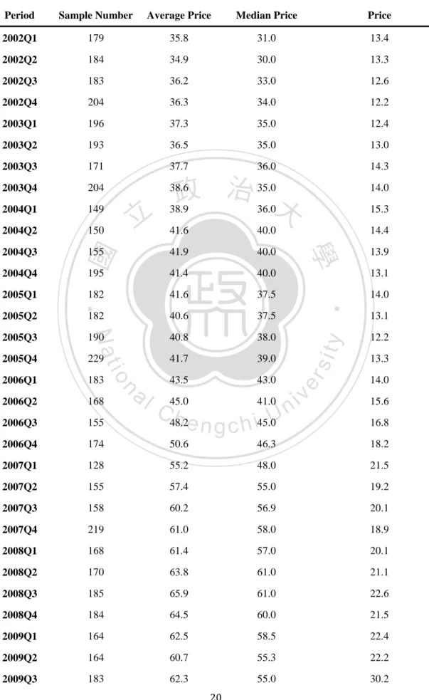
(19) Chapter 4. Data and Methodology. 4.1 Sample Description. The data I used for real estate marketing index collected the list price of the presale house and new house by developer in Taipei city from Wei Xin real estate magazine.. 政治大. Sample period is from 2001Q1 to 2014Q2 and the base period is 2006Q1. The total. 立. sample number are 7539, including 4038 presale house and 3501 new house samples.. ‧ 國. 學. As Table 1 showed, the average price increased consistently, average price rise 1.65. ‧. folds from 35.8 to 95.1, but slightly went down in 2008 and 2009. And I also observe. sit. y. Nat. io. n. al. er. median price have the same pattern, increased from 31 to 85, increasing 174%. i n U. v. appreciation, but slightly down trend in 2009. As a result, We can conclude there is. Ch. engchi. price uptrend at Taipei city from descriptive statistic. Moreover, we can find price standard deviation also rise up from 13.4 to 42.5. There are two possible explanation that the increased dwelling price cause price volatility up. Another is that the dispersion of developer’s list price increased, because different developer may provide different characteristic dwelling, which cause a variety of pricing strategies.. 19.

(20) Table 1. Descriptive Statistic of Sample. Period. Sample Number. Average Price. Median Price. Price. 2002Q1. 179. 35.8. 31.0. 13.4. 2002Q2. 184. 34.9. 30.0. 13.3. 2002Q3. 183. 36.2. 33.0. 12.6. 2002Q4. 204. 36.3. 34.0. 12.2. 2003Q1. 196. 37.3. 35.0. 12.4. 2003Q2. 193. 36.5. 35.0. 13.0. 2003Q3. 171. 37.7. 36.0. 14.3. 2003Q4. 204. 38.6. 35.0. 14.0. 2004Q1. 149. 38.9. 36.0. 15.3. 2004Q2. 150. 41.6. 40.0. 14.4. 2004Q3. 155. 41.9. 40.0. 195. 41.4. 40.0. 182. 41.6. 37.5. 182. 40.6. 37.5. ‧. 14.0. 2005Q2. ‧ 國. 2005Q3. 190. 40.8. 38.0. y. 12.2. 2005Q4. 229. 41.7. 39.0. sit. Standard Deviation of. 13.3. 2006Q1. 183. 43.5. 43.0. 2006Q2. 168. 45.0. 41.0. 2006Q3. 155. 2006Q4. 174. 50.6. 46.3. 18.2. 2007Q1. 128. 55.2. 48.0. 21.5. 2007Q2. 155. 57.4. 55.0. 19.2. 2007Q3. 158. 60.2. 56.9. 20.1. 2007Q4. 219. 61.0. 58.0. 18.9. 2008Q1. 168. 61.4. 57.0. 20.1. 2008Q2. 170. 63.8. 61.0. 21.1. 2008Q3. 185. 65.9. 61.0. 22.6. 2008Q4. 184. 64.5. 60.0. 21.5. 2009Q1. 164. 62.5. 58.5. 22.4. 2009Q2. 164. 60.7. 55.3. 22.2. 2009Q3. 183. 62.3. 55.0. 30.2. Nat. io. n. al. er. 2005Q1. 學. 2004Q4. 立. 政治大. i n U. C48.2 h e n g c h i45.0. 20. v. 13.9 13.1. 13.1. 14.0 15.6 16.8.

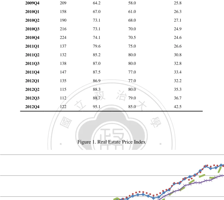
(21) 2009Q4. 209. 64.2. 58.0. 25.8. 2010Q1. 158. 67.0. 61.0. 26.3. 2010Q2. 190. 73.1. 68.0. 27.1. 2010Q3. 216. 73.1. 70.0. 24.9. 2010Q4. 224. 74.1. 70.5. 24.6. 2011Q1. 137. 79.6. 75.0. 26.6. 2011Q2. 132. 85.2. 80.0. 30.8. 2011Q3. 138. 87.0. 80.0. 32.8. 2011Q4. 147. 87.5. 77.0. 33.4. 2012Q1. 135. 86.9. 77.0. 32.2. 2012Q2. 115. 88.3. 80.0. 35.3. 2012Q3. 112. 88.7. 79.0. 36.7. 2012Q4. 122. 95.1. 85.0. 42.5. 立. y. sit. n. al. er. io. 2. 1.5. ‧. ‧ 國. 學 Figure 1. Real Estate Price Index. Nat. 2.5. 政治大. Ch. engchi. i n U. v. 1. 0.5. 2002Q1 2002Q2 2002Q3 2002Q4 2003Q1 2003Q2 2003Q3 2003Q4 2004Q1 2004Q2 2004Q3 2004Q4 2005Q1 2005Q2 2005Q3 2005Q4 2006Q1 2006Q2 2006Q3 2006Q4 2007Q1 2007Q2 2007Q3 2007Q4 2008Q1 2008Q2 2008Q3 2008Q4 2009Q1 2009Q2 2009Q3 2009Q4 2010Q1 2010Q2 2010Q3 2010Q4 2011Q1 2011Q2 2011Q3 2011Q4 2012Q1 2012Q2 2012Q3 2012Q4. 0. All sample. Presale house. 21. New house. Sinyi index.

(22) I construct the house price index, which is the proxy of futures index, by the method I mention last section. In addition, I want to separate the effect from presale house and new house. I construct price index based on three different data sets. The first one price index I formed by real estate marketing index (TAIALL) including all presale. 政治大. house and new house price. Next, I only use presales house price (PRESALE) to build. 立. up the presale house price index. Then, I formed the new house price index (NEW) only. ‧ 國. 學. by new house price data. By doing so, I can isolate the effect from different asset pool.. ‧. Also, I use the Sinyi house price index, which be published on Sinyi official website, as. sit. y. Nat. io. n. al. er. a spot market price index(SPOT). This index is composed of resale house price and. i n U. v. constructed by hedonic price method, sample periods cover from 2001Q1 to 2013Q1.. Ch. engchi. Base period is 2001Q1. To make the data in a consistent basis, I normalize Sinyi Index to 2006Q1, which is the same base period as real estate marketing Index. As figure 1 presented, I can observe all of four price indexes show strong upturn.. 22.

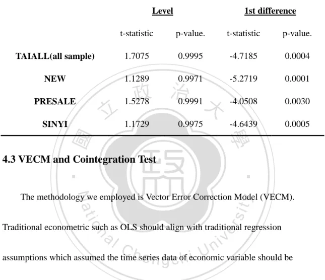
(23) 4.2 Unit-Root. Moreover, I did unit-root test for All, Presale, New and Sinyi index, because I applied the time-series model which assumes that time series data have to be stationary. Therefore, I use Augmented Dickey-Fuller(ADF) method to test the unit-root. 𝑝. ∆𝑌𝑡 = 𝑎0 + 𝑟𝑌𝑡−1 + 𝑎2 𝑡 + ∑ 𝛽∆𝑌𝑡−𝑖+1 + 𝜀𝑡. 政治大 𝑖=2. 立. According to ADF test, the null hypothesis is that the time series data are not. ‧ 國. 學. stationary and alternative hypothesis is that time series data are stationary. If we can. al. y. sit. io. 𝐻𝑎 : 𝑟 < 0, unit root do not exist. er. Nat. 𝐻0 : 𝑟 = 0, unit root exist. ‧. reject 𝐻0 then we can say the time series data is stationary.. n. v i n C h of unit-root test. As The following table 2 are results e n g c h i U the table5 showed, we can observe that those four indexes are not stationery. Their p-value all above 0.99, it also means we can not reject null hypothesis, so the data have unit-root. In addition, we can watch figure.1 that all the four indexes represent uptrend consistently without any downtrend and do not revert to long term equilibrium, we also can say they are not stationary from figure 1. To resolve this problem, we took 1st difference then did the ADF test. The property of unit-root is eliminated. All the p-value are below 0.01, 23.

(24) therefore, we can reject null hypothesis and have sufficient evidence to say the time series data are stationary after 1st differenced. Table 2. Result of Augmented Dickey-Fuller Test Level. 1st difference. t-statistic. p-value.. t-statistic. p-value.. TAIALL(all sample). 1.7075. 0.9995. -4.7185. 0.0004. NEW. 1.1289. 0.9971. -5.2719. 0.0001. PRESALE. 1.5278. -4.0508. 0.0030. -4.6439. 0.0005. 立. SINYI. 政治 0.9991 大. 1.1729. 0.9975. ‧ 國. 學. 4.3 VECM and Cointegration Test. ‧. Nat. er. io. sit. y. The methodology we employed is Vector Error Correction Model (VECM). Traditional econometric such as OLS should align with traditional regression. n. al. Ch. engchi. i n U. v. assumptions which assumed the time series data of economic variable should be stationary and residuals should be non-serial correlation. In general, most of economic variables are non-stationary. If we find that the variables are not stationary after unit-root test, there are two ways to resolve the problem. First, we can eliminate the deterministic trend of the economic variable. Second, you can eliminate stochastic trend by difference which is the most simplest and common way. However, data may lose long term information after difference. Therefore, Engle and Granger (1987) proposed 24.

(25) the cointegration concept to resolve this problem. The concept of cointegration applies to a wide variety of economic models. Any equilibrium relationship among a set of non-stationary variables implies that their stochastic trend must be linked. After all, the equilibrium relationship means that the variables cannot move independently of each other. This linkage among the stochastic trends necessitates that the variables be. 政治大. cointegrated and there is a linear relationship among the variables. Since the. 立. cointegrated variables are linked, there are two types of change when the economic. ‧ 國. 學. variables varying. One is temporal another is permanent. Permanent change is the. ‧. change of long trend which is low frequencies. And temporal change is that the dynamic. sit. y. Nat. io. n. al. er. pahts of such variables must bear some relation to the current deviation from the. i n U. v. equilibrium relationship by some reasons but it will back to long term equilibrium. Ch. engchi. during the time passing. Engle and Granger (1987) provided famous Granger Representation which stated two major concepts. First, an error correction model for I(1) variables necessarily implies cointegration. Second, It can also be shown that cointegration implies error correction. Therefore, when two variables exist cointegrated relationship, they expressed as error correction model. To test cointrgration relationship, I can use Engle and Granger two steps cointegration test processing. Step 1, If both of 25.

(26) variables are unit-root and I(1) series, then we can use OLS to compute its residual. Step 2, To test the residuals whether it exists unit-root, if there is unit-root then we will say both of two variable are not integrated. On the other hand, if the residual do not exist unit-root then both of variables are cointegrated. I also can use the rank of π to determine whether or not the variables in 𝑥𝑡 are integrated. To elaborate, consider the simple case of a first order VAR:. 立. 政治大 𝑥𝑡 = 𝐴1 𝑥𝑡−1 + 𝜀𝑡. ‧ 國. 學. Where 𝑥𝑡 is the (n x 1) vector (𝑥1𝑡, 𝑥2𝑡, … 𝑥𝑛𝑡 ). 𝜀𝑡 is the (n x 1) vector. ‧. (𝜀1𝑡, 𝜀2𝑡, … 𝜀𝑛𝑡 ). 𝐴1 is an (n x n) matrix of parameters. Subtracting from each side of. sit. y. Nat. io. n. al. er. the equation, we get. i n U. v. ∆𝑥𝑡 = −(𝐼 − 𝐴1 )𝑥𝑡−1 + 𝜀𝑡 = 𝜋𝑥𝑡−1 + 𝜀𝑡. Ch. engchi. If the rank of π matrix is zero, each element of it must equal zero. In this instance, the equation is equivalent to an n-variable VAR in first differences: ∆𝑥𝑡 = 𝜀𝑡 All the {𝑥𝑡 } sequences are unit-root processes and there is no linear combination of the variable which is stationary. At the other extreme, suppose that π is of full rank The long-run solution to dynamic system is given by the n independent equations: 26.

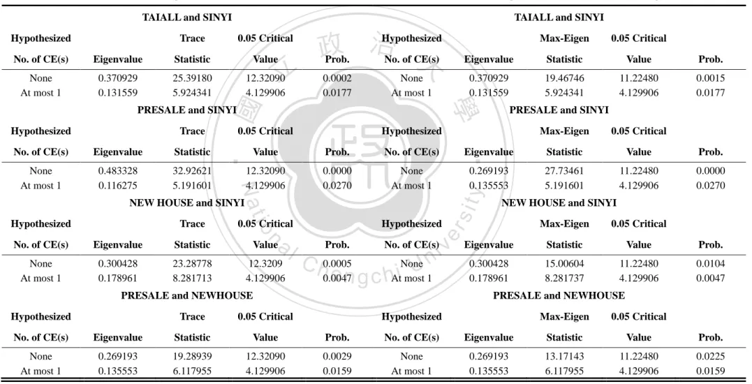
(27) 𝜋11 𝑥1𝑡 − 𝜋12 𝑥2𝑡 + 𝜋13 𝑥3𝑡 + ⋯ + 𝜋1𝑛 𝑥𝑛𝑡 = 0 𝜋21 𝑥1𝑡 − 𝜋22 𝑥2𝑡 + 𝜋23 𝑥3𝑡 + ⋯ + 𝜋2𝑛 𝑥𝑛𝑡 = 0 𝜋𝑛1 𝑥1𝑡 − 𝜋𝑛2 𝑥2𝑡 + 𝜋𝑛3 𝑥3𝑡 + ⋯ + 𝜋𝑛𝑛 𝑥𝑛𝑡 = 0 In this case, each of the n variables contained in the vector must be stationary with the long-run values given by solving the above system. In this paper, I use the Johansen cointegration method to test the conintergration. We know from linear algebra that the rank of a matrix is equal to the number of non-zero characteristic roots. Therefore, the. 政治大 number of distinct co-integrating vectors can be obtained by checking the significance 立. ‧ 國. 學. of the characteristic roots of π . The following table is the Johansen test results. I. ‧. assumed that there is no intercept or trend in CE or test VAR. As the result represented,. Nat. er. io. sit. y. the TAIALL and Sinyi index significantly exist at most 1 cointegration relationship under the trace and maximum eigenvalue method. The presale house and Sinyi also. n. al. Ch. engchi. i n U. v. have at most 1 cointegration relationship under the trace and maximum eigenvalue method. The conintegration test of new house and Sinyi represented a conintergration pattern which p-value are 0.0005 under trace method and 0.0104 under maximum eigenvalue method. And even presale and new house represented a significant cointegration relationship. After cointegration test, we can conclude that all of the variables exist cointegration. Therefore, I can employ VECM model to test the price lead-lag relationship. 27.

(28) Table 3. Johnansen Cointegration Test Unrestricted Cointegration Rank Test (Trace). Unrestricted Cointegration Rank Test (Maximum Eigenvalue). TAIALL and SINYI. TAIALL and SINYI. Trace. 0.05 Critical. No. of CE(s). Eigenvalue. Statistic. Value. None At most 1. 0.370929 0.131559. 25.39180 5.924341. 12.32090 4.129906. 立. 政治大. Hypothesized Eigenvalue. Statistic. Value. Prob.. 0.0002 0.0177. None At most 1. 0.370929 0.131559. 19.46746 5.924341. 11.22480 4.129906. 0.0015 0.0177. Statistic. None At most 1. 0.483328 0.116275. 32.92621 5.191601. Hypothesized. Value. Prob.. No. of CE(s). 12.32090 4.129906. 0.0000 0.0270. None At most 1. NEW HOUSE and SINYI. 0.05 Critical. n. al. No. of CE(s). Eigenvalue. Statistic. Value. None At most 1. 0.300428 0.178961. 23.28778 8.281713. 12.3209 4.129906. Hypothesized. v i n. Prob.. No. of CE(s). C h0.0005 None U1 i e n g c hAt most 0.0047. PRESALE and NEWHOUSE Hypothesized. Trace. 0.05 Critical. 0.05 Critical. Eigenvalue. Statistic. Value. Prob.. 0.269193 0.135553. 27.73461 5.191601. 11.22480 4.129906. 0.0000 0.0270. NEW HOUSE and SINYI Max-Eigen. 0.05 Critical. Eigenvalue. Statistic. Value. Prob.. 0.300428 0.178961. 15.00604 8.281737. 11.22480 4.129906. 0.0104 0.0047. er. Trace. io. Hypothesized. Max-Eigen. y. Eigenvalue. Nat. No. of CE(s). 0.05 Critical. PRESALE and SINYI. ‧. ‧ 國. 學. Trace. 0.05 Critical. No. of CE(s). PRESALE and SINYI Hypothesized. Max-Eigen. Prob.. sit. Hypothesized. PRESALE and NEWHOUSE Hypothesized. Max-Eigen. 0.05 Critical. No. of CE(s). Eigenvalue. Statistic. Value. Prob.. No. of CE(s). Eigenvalue. Statistic. Value. Prob.. None At most 1. 0.269193 0.135553. 19.28939 6.117955. 12.32090 4.129906. 0.0029 0.0159. None At most 1. 0.269193 0.135553. 13.17143 6.117955. 11.22480 4.129906. 0.0225 0.0159. 28.

(29) For a VECM model, first, we considered a VAR(p) model: ∆𝑦𝑡 = 𝑚 + 𝐴1 𝑦𝑡−1 + 𝐴2 𝑦𝑡−2 + ⋯ + 𝐴𝑝 𝑦𝑡−𝑝 + 𝜀𝑡 , 𝜀𝑡 ~𝑊𝑁(0, Ω) According to Granger Representation theorem, VAR(p) model can be expressed to vector error correlation model: 𝑝−1. Δ𝑦𝑡 = 𝑚 + ∑ 𝐵𝑗 ∆𝑦𝑡−𝑗 − 𝛼𝛽 ′ 𝑦𝑡−1 + 𝜀𝑡 𝑗=1. 政治大 =立 𝑚 + ∑ 𝐵 ∆𝑦 − ∏𝑦 + 𝜀 𝑝−1. 𝑗. 𝑡−𝑗. 𝑡−1. 𝑡. 𝑗=1. ‧ 國. 學. If ∆𝑦𝑡 , ∑𝑝−1 𝑗=1 𝐵𝑗 ∆𝑦𝑡−𝑗 and 𝜀𝑡 are all stationery.Then ∏𝑦𝑡−1 must be stationery too.. ‧. In this model, ∏ = α𝛽 ′ , Both α and β are k × r matrix. It evaluated long term effect.. y. Nat. n. er. io. al. sit. And 𝐵𝑗 evaluated short term effect.. i n U. v. To study the price lead-lag relationship between spot and futures, I applied the VECM model as follow:. Ch. engchi. 𝐸𝑞 1 ∶ 𝑒𝑐𝑚 ̂ 𝑡−1 = 𝛼0 + 𝐹𝑡−1 + 𝛼1 𝑆𝑡−1 𝐸𝑞 2 ∶ ∆𝐹𝑡 = 𝛽0 + 𝛽1 𝑒𝑐𝑚 ̂ 𝑡−1 + 𝛽2 ∆𝐹𝑡−1 + 𝛽3 ∆𝑆𝑡−1 + 𝛽4 ∆𝐹𝑡−2 + 𝛽5 ∆𝑆𝑡−2 + 𝛽6 𝑅𝑎𝑡𝑒𝑡 + 𝛽7 ln(𝐺𝐷𝑃𝑝𝑒𝑟)𝑡 + 𝛽8 ln(𝑆𝑡𝑜𝑐𝑘)𝑡 𝐸𝑞 3 ∶ ∆𝑆𝑡 = 𝛽0 + 𝛽1 𝑒𝑐𝑚 ̂ 𝑡−1 + 𝛽2 ∆𝐹𝑡−1 + 𝛽3 ∆𝑆𝑡−1 + 𝛽4 ∆𝐹𝑡−2 + 𝛽5 ∆𝑆𝑡−2 + 𝛽6 𝑅𝑎𝑡𝑒𝑡 + 𝛽7 ln(𝐺𝐷𝑃𝑝𝑒𝑟)𝑡 + 𝛽8 ln(𝑆𝑡𝑜𝑐𝑘)𝑡 29.

(30) Here, Eq1 represented long term equilibrium equation. Eq2 and Eq3 showed short term equilibrium equation. Also, We can transform the model into reduced form like: ∆𝐹𝑡 = (𝛽0 + 𝛼0 𝛽1 ) + 𝛽1 𝐹𝑡−1 + 𝛼1 𝛽1 𝑆𝑡−1 + 𝛽2 ∆𝐹𝑡−1 + 𝛽3 ∆𝑆𝑡−1 + 𝛽4 ∆𝐹𝑡−2 + 𝛽5 ∆𝑆𝑡−2 + 𝛽6 𝑅𝑎𝑡𝑒𝑡 + 𝛽7 ln(𝐺𝐷𝑃𝑝𝑒𝑟)𝑡 + 𝛽8 ln(𝑆𝑡𝑜𝑐𝑘)𝑡 ∆𝑆𝑡 = (𝛽0 + 𝛼0 𝛽1 ) + 𝛽1 𝐹𝑡−1 + 𝛼1 𝛽1 𝑆𝑡−1 + 𝛽2 ∆𝐹𝑡−1 + 𝛽3 ∆𝑆𝑡−1 + 𝛽4 ∆𝐹𝑡−2. 政治大. + 𝛽5 ∆𝑆𝑡−2 + 𝛽6 𝑅𝑎𝑡𝑒𝑡 + 𝛽7 ln(𝐺𝐷𝑃𝑝𝑒𝑟)𝑡 + 𝛽8 ln(𝑆𝑡𝑜𝑐𝑘)𝑡. 立. In my studies, ∆F is 1st difference of the proxy futures price index at time t, ∆S is. ‧ 國. 學. 1st difference of the proxy of spot price index at time t, ln(GDPPER) is exponential. ‧. logarithmic of GDP per capita, ln(STOCK) is exponential logarithmic of TAIEX, RATE. sit. y. Nat. io. n. al. er. is residential mortgage borrowing rate. Sample period is 2002Q1 to 2012 Q4. Using this. i n U. v. equation, I test the price lead-lag relationship for my experimenta. Ch. engchi. 30.

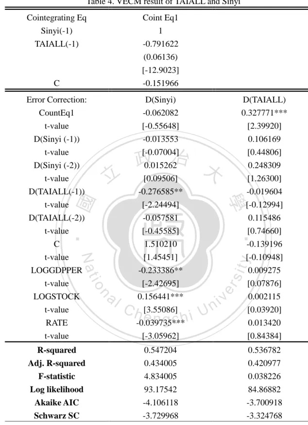
(31) Chapter 5. Empirical Result The VECM results are showed as following tables. First, I use all sample data including presale and new house to test the price lead-lag relationship with Sinyi index. The result represented on the Table 4. First, we can find a significant long term conintegration relationship between TAIALL and Sinyi index t value is -12.9023. It. 政治大. means the Sinyi index will increase 0.7916 when TAIALL increases 1 unit in long term. 立. equilibrium. Also, We also find correction term is significant which t value is 2.39920 in. ‧ 國. 學. D(TAIALL). When Sinyi index is high and deviated from long term equilibrium, the. ‧. TAIALL will adjust its price higher to the long term equilibrium relationship. The speed. sit. y. Nat. io. n. al. er. of adjustment in TAIALL will be faster than Sinyi. Therefore, we can say the TAIALL. i n U. v. leads the resale market because developers have more information to forecast the price. Ch. engchi. trend of real estate market compared to resident buyer. The result coincides the hypothesis one. In the short term perspectives, the 1st difference of TAIALL have a negative price adjustment in Sinyi which t value is -2.2494. The resale price will rise when the real estate marketing index goes down in short adjustment. The coefficient of RATE is significantly negative, which is -0.039735. It means that when the rate is low, the second hand house market price will be spurred by cheaper capital. Also, resale 31.

(32) Table 4. VECM result of TAIALL and Sinyi Cointegrating Eq Sinyi(-1) TAIALL(-1). C. Coint Eq1 1 -0.791622 (0.06136) [-12.9023] -0.151966. Error Correction: CountEq1. D(Sinyi) -0.062082. D(TAIALL) 0.327771***. t-value D(Sinyi (-1)) t-value D(Sinyi (-2)) t-value D(TAIALL(-1)) t-value D(TAIALL(-2)) t-value C. [-0.55648] -0.013553 [-0.07004] 0.015262 [0.09506] -0.276585** [-2.24494] -0.057581 [-0.45585] 1.510210. [2.39920] 0.106169 [0.44806] 0.248309 [1.26300] -0.019604 [-0.12994] 0.115486 [0.74660] -0.139196. n. Ch. engchi. y. [-0.10948] 0.009275 [0.07876] 0.002115 [0.03920] 0.013420 [0.84384]. sit er. io. al. [1.45451] -0.233386** [-2.42695] 0.156441*** [3.55086] -0.039735*** [-3.05962]. ‧. Nat. t-value LOGGDPPER t-value LOGSTOCK t-value RATE t-value. 學. ‧ 國. 立. 政治大. i n U. v. R-squared Adj. R-squared F-statistic. 0.547204 0.434005 4.834005. 0.536782 0.420977 0.038226. Log likelihood Akaike AIC Schwarz SC. 93.17542 -4.106118 -3.729968. 84.86882 -3.700918 -3.324768. *,**, and *** Singnificant at 10%, 5% and 1% levels, respectively. 32.

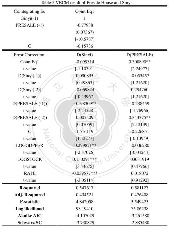
(33) house is influenced significantly by stock market. The Sinyi price index movement aligns with stock market, it may be because people have more money to spend driving house price increased. While, the GDPPER variable is -0.233386, it means when GDP per capita goes down, the house price goes up. It obeys normal understanding which price will be higher when people become rich. There may be a possible explanation that. 政治大. house price deviated from fundamental demand.. 立. Then, we separated all samples into two groups, presale and new house, to isolate. ‧ 國. 學. two different markets features. Table 5 showed the result of presale house. We can see. ‧. the same result that there is a significant cointegration relationship between Sinyi and. sit. y. Nat. io. n. al. er. PRESALE which t value is -10.5787. According to the correction term, the presale. i n U. v. market correction the price discrepancies when deviating the long equilibrium. We can. Ch. engchi. find a significant lead-lag relationship that the speed of price adjustment of future market leads spot market. It aligns with our hypothesis one which the market participants with more information will reflect the price fast. Also, we can observe the same result in short term perspectives. There is a significantly negative adjustment in Sinyi index by D(PRESALE(-1)) which t value is -2.24598. And presale market is influenced significantly by its first and second order lag term which net effect positive. 33.

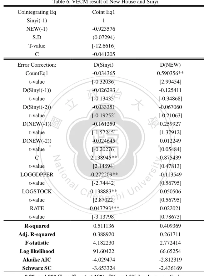
(34) It means there is a short term momentum that the high price of presale house will drive the price higher in the next period. Also, we can explain all of developers act at the same direction. The stock and rate variables represented the same pattern in explaining resale market as previous result. The stock variable is significantly positive and the rate variable significantly negative. The coefficient of gdpper is -0.229821, also significant.. 政治大. In new house, we can see the table 6 that we can find that there is also a. 立. cointegration relationship between Sinyi and NEW. As a result, the new house market. ‧ 國. 學. leads the resale market too in the long term perspectives. The developers take the price. ‧. advantage in pricing. If the price deviated form long term equilibrium then developer. sit. y. Nat. io. n. al. er. will adjust the price of new house first. The result also met our hypothesis one. None of. i n U. v. short term adjusted variables are significant. There is no short term price adjustment. Ch. engchi. between Sinyi and NEW. The possible explanation is that the new house and second house are largely homogeneous. The price movement in new house and resale market follow the same pattern. The feature causes an insignificant short term. 34.

(35) Table 5.VECM result of Presale House and Sinyi Cointegrating Eq Sinyi(-1) PRESALE (-1). C. Coint Eq1 1 -0.77938 (0.07367) [-10.5787] -0.15736. Error Correction:. D(Sinyi). D(PRESALE). CountEq1 t-value D(Sinyi(-1)) t-value. -0.099314 [-1.10391] 0.090895 [0.49863]. 0.308890** [2.24977] -0.055457 [1.21620]. -0.069824 [-0.43967] -0.198309** [-2.24598] 0.007509 [0.07059]. 0.294760 [1.21620] -0.238459 [-1.76966] 0.344375** [2.12139]. engchi. y. -0.226851 [-0.13949] -0.006280 [-0.04244] 03031919 [0.47966] 0.018072 [0.91292]. sit. ‧ 國 n. Ch. ‧. io. al. 1.516119 [1.42277] -0.229821** [-2.37026] 0.150291*** [3.44675] -0.039577*** [-3.05114]. 學. Nat. C t-value LOGGDPPER t-value LOGSTOCK t-value RATE t-value. er. 立. D(Sinyi(-2)) t-value D(PRESALE (-1)) t-value D(PRESALE (-2)) t-value. 政治大. i n U. v. R-squared Adj. R-squared. 0.547617 0.434521. 0.581127 0.476408. F-statistic Log likelihood Akaike AIC Schwarz SC. 4.842058 93.19410 -4.107029 -3.730879. 5.549425 75.86238 -3.261580 -2.885430. *,**, and *** Singnificant at 10%, 5% and 1% levels, respectively. 35.

(36) Table 6. VECM result of New House and Sinyi Cointegrating Eq Sinyi(-1) NEW(-1) S.D T-value C. Coint Eq1 1 -0.923576 (0.07294) [-12.6616] -0.041205. Error Correction:. D(Sinyi). D(NEW). CountEq1 t-value D(Sinyi(-1)) t-value D(Sinyi(-2)) t-value D(NEW(-1)) t-value D(NEW(-2)) t-value. -0.034365 [-0.32036] -0.026293 [-0.13435] -0.033351 [-0.19252] -0.161259 [-1.57245] -0.024645 [-0.20276]. 0.590356** [2.99454] -0.125411 [-0.34868] -0.067060 [-0.21063] 0.259927 [1.37912] 0.012249 [0.05484]. n. Ch. engchi. y. 0.875439 [0.47813] -0.113549 [0.56795] 0.050506 [0.56795] 0.022021 [0.78673]. sit er. io. al. 2.138945** [2.14694] -0.272209** [-2.74442] 0.138883** [2.87022] -0.047793*** [-3.13798]. ‧. Nat. C t-value LOGGDPPER t-value LOGSTOCK t-value RATE t-value. 學. ‧ 國. 立. 政治大. i n U. v. R-squared Adj. R-squared. 0.511136 0.388920. 0.409369 0.261711. F-statistic Log likelihood Akaike AIC Schwarz SC. 4.182230 91.60422 -4.029474 -3.653324. 2.772414 66.65254 -2.812319 -2.436169. *,**, and *** Singnificant at 10%, 5% and 1% levels, respectively. 36.

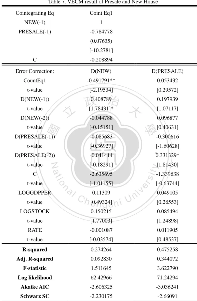
(37) relationship between two markets. The stock and rate variables showed consistent significantly consequence with pervious results, which coefficient are 0.138883, -0.047793. And the variable of GDPPER is -0.272209, also significant. After separating all samples into two different markets, We can find the future market still leads the spot market at each group. In the presales market, there is a short. 政治大. term momentum of presale market. However, the short term relationship of price. 立. adjustment was disappeared in new house sample because its homogenous features.. ‧ 國. 學. Here, I also test the price relationship between new house and presale house. In. ‧. both of markets, Developers decide the listing price. The result represented on table 7.. sit. y. Nat. io. n. al. er. There is also a significant cointegration between new house and presale. However, in. i n U. v. the table 7, we can observe the correction term is significantly negative in the new. Ch. engchi. house market. Therefore, as developers’ view, when the price of new house is high and away from long run equilibrium, the developers will revise the price of new house down rather than presale because the carrying cost of new house is high and it will tight developers’ capital. So, we can say the new house market will lead presale market when the price away from long run equilibrium. The result aligns our hypothesis two which participants with higher carrying cost will reflect price fast. Also, the new house price 37.

(38) index is influenced positive by its lag term which t value is 1.78431. There is a short term momentum like presale market. And the stock positively explained the spot market.. 立. 政治大. ‧. ‧ 國. 學. n. er. io. sit. y. Nat. al. Ch. engchi. 38. i n U. v.

(39) Table 7. VECM result of Presale and New House Cointegrating Eq. Coint Eq1. NEW(-1). 1. PRESALE(-1). -0.784778 (0.07635) [-10.2781]. C. -0.208894. Error Correction:. D(NEW). D(PRESALE). CountEq1. -0.491791**. 0.053432. t-value. [-2.19534]. [0.29572]. D(NEW(-1)) t-value. 0.197939. t-value. [-0.15151]. [0.40631]. D(PRESALE(-1)). -0.085683. t-value. [-0.36927]. D(PRESALE(-2)). -0.041414. t-value. [-0.18291] -2.635695. t-value LOGSTOCK. al. n. LOGGDPPER. io. t-value. [-1.01155] 0.11309. C h [0.49324] engchi. [-1.60628] 0.331329* [1.81430]. -1.339638. er. Nat. C. -0.300616. ‧. ‧ 國. 0.096877. 學. -0.044788. y. [1.07117]. sit. 立. D(NEW(-2)). 0.408789 治政大 [1.78431]*. i n U. v. [-0.63744] 0.049105 [0.26553]. 0.150215. 0.085494. t-value. [1.77003]. [1.24898]. RATE. -0.001087. 0.011905. t-value. [-0.03574]. [0.48537]. R-squared. 0.274264. 0.475258. Adj. R-squared. 0.092830. 0.344072. F-statistic. 1.511645. 3.622790. Log likelihood. 62.42966. 71.24294. Akaike AIC. -2.606325. -3.036241. Schwarz SC. -2.230175. -2.66091. *,**, and *** Singnificant at 10%, 5% and 1% levels, respectively 39.

(40) Chapter 6. Conclusion According to our VECM results, We can find that there is a cointegration relationship between real estate marketing index and Sinyi price index. And the speed of price adjustment is faster in the marketing index when the price relationship deviate from long term conintegration. It matchs our first hypothesis which is developers take. 政治大. information advantage. In the short term, the marketing index lead resale market. For. 立. presale and resale market, the presale leads resale market in both of short and long run.. ‧ 國. 學. Also, there is short term momentum in presale market. It means developers will follow. ‧. market momentum such as chase the high price at good market. Also, the listing price of. sit. y. Nat. io. n. al. er. new house also leads the resale house in the short and long run. There is a price momentum as the same as presale market.. Ch. engchi. i n U. v. However, when we focus on the presale market and new house, the new house leads presale in the long run equilibrium. The reason is that the carrying cost of presale house is less than new house which match our hypothesis two. So, developer would like adjust the price of new house rather than presale because the carry cost concern. Finally, the macro variables are significant in explaining Sinyi index. The rate is negative significantly in resale because resale house buyer will be affected directly by 40.

(41) the mortgage borrowing rate. The stock variables also showed the capital market will influence resale market significantly. But we don’t whether the resale market affect stock market too. In the end, the GDP variable is significantly negative, the reason may be the house of resale house has away from residents demand.. 立. 政治大. ‧. ‧ 國. 學. n. er. io. sit. y. Nat. al. Ch. engchi. 41. i n U. v.

(42) Reference 1. Blose, Laurence E., 2010, “Gold prices, cost of carry, and expected inflation”, Journal of Economics and Business, 62, 35-47 2. Chau, K. W., Wong, S. K. and Yiu, C. Y., 2009, “Transaction volume and price dispersion in presale and spot real estate markets”, Journal of Real Estate Finance and Economics, 38, 241-253 3. Chau, K. W., Wong, S. K. and Yiu, C. Y., 2007, “Volatility transmission in the real estae spot and forward markets”, Journal of Economics and Business, 35, 281-293 4. Chau, K. W., Wong, S. K. and Yiu, C. Y., 2007, “Housing quality in the Forward Contracts Market”, Journal of Real Estate Finance and Economics, 34, 313-325. 治政 stock index futures market. ”, The Review of Financial Studies, 大 5, 123-152 Diamond, Douglas W. and立 Verrecchia, Robert E., 1987, “Constraints on short-selling and. 5. Chan, K., 1992, “A further analysis of the lead-lag relationship between the cash market and. 6.. ‧ 國. 277-311. 學. asset price adjustment to private information”, The Journal of Finance Economics, 18,. ‧. 7. Fisher, J., Gatzlaff, D. and Geltner, D. 2004, “An analysis of the determinants of transaction frequency of institutional commercial real estate investment property”, Real Estate. sit. y. Nat. Economics, 32, 239-264. 8. Gyourko, Joseph and Keim, Donald B., 1992, “What does the stock market tell us about real. io. al. n. v i n C Indexes for Housing U Hill, Robert, 2011, “Hedonic Price h e n g c h i ”, OECD Statistics Working Papers. 20(3), 457-485 9.. er. estate returns” Journal of the Americam Real Estate and Urban Economics Association,. 10. Heaney, Richard, 1998, “A test of the cost-of-carry relationship using the London metal exchange lead contract.” The Journal of Futures Markets, 18, 177-200 11. Hort, Katinka, 2000, “Price and turnover in the market for owner-occupied homes”, Regional Science and Urban Economics, 30, 99-119 12. Ibbotson, Roger G. and Siegel, Laurence B., 1984, “Real estate return: A comparison with other investment”, Real Estate Economic, 12, 219-242 13. Joseph T, L. Ooi. And Thao T. T. Le, 2012, “New supply and price dynamics in the Singapore housing market”, Urban Studies, 49, 1435-1451 14. Modest, David M., Sundaresan, Mahadevan, 1983, “The relationship between spot and futures prices in stock index futures markets: some preliminary evidence”, The Journal of Futures Markets, 3(1), 15-41 42.

(43) 15. Martin, J. Bailey, Richard, F. Muth and Hugh O. Nourse, 1963, “A regression method for real estate price index construction”, Journal of American Statistical Associatioin, 58, 933-942 16. Sarno, Lucio and Valente, Giorgio, 2000, “The cost of carry model and regime shifts in stock index futures markets: an empirical investigation”, The Journal of Futures Markets, 20, 603-624 17. Stephan, Jens A. and Whaley, Robert E., 1990, “Intraday price change and trading volume relations in stock and stock option markets.” The Journal of Finance, 45(1), 191-220 18. Stein, Jeremy C. 1995, “The prices and Trading Volume in the Housing Market: A model with down-payment effects”, The Quarterly Journal of Economics”, 110, 379-406 19. Yiu, C. Y., Hui, E. C. M. and Wong, S. K., 2005, “Lead-Lag Relationship between the Real. 政治大. Estate Spot and Forward Contracts Market”, Journal of Real Estate Portfolio Management,. 立. 11, 253-262. 20.張麗姬 (民 83)，「從遠期契約和現貨的角度論預售屋和成屋的價格關係─以台. ‧ 國. 學. 北市為例」，住宅學報，第二期，第 67-85 頁. 21.張金鶚、楊宗憲、洪裕仁 (民 97)，「中古屋及預售屋房價指數之建立、評估與. ‧. 整合─以台北市之實證分析」，住宅學報，第二期，第 13-34 頁. n. er. io. sit. y. Nat. al. Ch. engchi. 43. i n U. v.

(44)