A self-learning fault diagnosis system based on reinforcement learning

(1)

Subscriber access provided by NATIONAL TAIWAN UNIV

Industrial & Engineering Chemistry Research is published by the American Chemical Society. 1155 Sixteenth Street N.W., Washington, DC 20036

A self-learning fault diagnosis system based on reinforcement learning

Yih Yuan Hsu, and Cheng Ching Yu

Ind. Eng. Chem. Res., 1992, 31 (8), 1937-1946 • DOI: 10.1021/ie00008a015 Downloaded from http://pubs.acs.org on November 28, 2008

More About This Article

The permalink http://dx.doi.org/10.1021/ie00008a015 provides access to: • Links to articles and content related to this article

(2)

Ind. Eng. Chem. Res. 1992,31,1937-1946

A

Self-Learning Fault Diagnosis System Based

on

Reinforcement

Learning

1937

Yih-Yuan Hsu and Cheng-Ching

Yu*

Department of Chemical Engineering, National Taiwan Institute of Technology, Taipei, Taiwan 106, R.O.C. In recent years, the evolution of qualitative physics has lead to the rapid development of deep- model-based diagnostic systems. Yu and Lee integrated quantitative process knowledge into a deep-model-based diagnostic system. In the qualitative/quantitative knowledge-based systems, the qualitative model and approximated numerical values are needed to construct a diagnostic system. This results in a bottleneck in the knowledge-acquisition step. On the other hand, another branch in artificial intelligence, artificial neural network (ANN), has the advantage of self-learning. This

work utilizes the self-learning feature of the ANN such that the semiquantitative knowledge can

be integrated into the qualitative/quantitative model in the learning steps. A chemical reactor example is used to illustrate the advantages of the proposed diagnostic system. Simulation results show that the proposed diagnostic system not only

has

the self-learning ability of ANN but also

is transparent to the users. Moreover, it does not produce erroneous solutions when compared with the backpropagation ANN and it also gives less spurious solutions when compared with qualitative model-based systems.

1. Introduction

In recent years, the complexity of modern chemical plants and the availability of inexpensive computer hardware prompted us to develop automated fault diagnosis instead of conventional diagnosis by the operator (Himmelblau, 1978; Isermann, 1984; Frank, 1990). Gen- erally, depending on the rigorousness of the process knowledge employed, techniques for automated fault diagnosis can be classified into qualitative, qualitative/ quantitative, and quantitative approaches. The qualitative approach only considers the signs of coefficients in all governing equations of process variables. The signed directed graph (SDG) is a typical example. Upon diagnosis, the consistency of the branches of a given fault origin is checked to validate (or invalidate) this hypothesis and all possible fault origins are screened. In many cases, it simply gives multiple interpretations for a single event (Kramer and Palowitch, 1987; Chang and Yu, 1990).

This

is an inherent limitation of the qualitative model-based systems. Since only qualitative knowledge is employed, the diagnostic resolution can only be improved to a certain degree. The quantitative model-based diagnostic systems, on the other hand, utilize the process model and on-line measurements to back-calculate crucial process variables. It finds the fault origins according to the perturbations in the calculated variables (Willsky, 1976; Isermann, 1984; Petti et al., 1990). Generally, this approach is too time- consuming and requires a significant amount of modeling effort. Originated from the artificial neural network

(ANN),

the backpropagation neural network is often employed in fault diagnosis (Watanabe et al., 1989). Gen- erally, this type of approach can also be classified as a quantitative model-based diagnostic system. It utilizes a set of process data, such as the values of steady-state process variables for the nominal operating condition and these for the identified faulty conditions, to train the network (Watanabe et al., 1989; Venkatasubramanian et al., 1990; Ungar et al., 1990). Following the training, the model is established and ready for fault diagnosis. Despite its black-box nature, the backpropagation neural network can accurately pin down the fault origin in most cases. Unfortunately, the parameters (such as input variables,

*

To whom correspondence should be addressed.

0SSS-5~5/92/263~-1937$03.O0/0

number of processing elements, and learning constants) must be determined by trial and error. If thew parameters are not chosen adequately, the convergence of the network can be difficult and erroneous interpretations may result. Another approach is the qualitative/quantitative mod- el-baaed diagnostic system. Yu and Lee (1991) integrated semiquantitative knowledge (e.g., steady-state gains) into a deep model-based diagnostic system to improve diagnostic resolution. One advantage of this approach is that the semiquantitative knowledge is added to a qualitative model (structure). The approach of Yu and Lee is similar, in concept, to the approaches of data interpretation (Cheung and Stephanopoulos, 1990a,b; Praaad and Davis, 1991; Rengaswamy and Venkatasubramanian, 1992) which received quite a bit attention recently. The data interpretation approaches devise a mechanism to map from quantitative data to qualitative interpretations which can

then be used by some appropriate qualitative (or semiquantitative) models. However, these two approaches differ significantly in defining the boundary between the model and input to the model. In data interpretation, quantitative data are transformed to qualitative (or semiquantitative) interpretations for corresponding models.

As

for the approach of Yu and Lee (1991), the quantitative data are plugged directly into the semiquantitative model to check the consistency. Regardless of the approaches employed, the semiquantitative knowledge has to be modified as the operating condition changes. This can lead to a knowledge-acquisition bottleneck in any realistic application. Therefore, an efficient method to acquire aem- iquantitative knowledge is necessary for fault diagnosis in the chemical process industries.

An ideal diagnostic system should have at least the following properties:

Soundness (Kuipers, 1988): Regardless of the number of the spurious solutions, it cannot have any erroneous solution (i.e., the true fault origin is not included in the solution set) at different operating conditions.

Transparency: The model should be easy to understand and the knowledge base, e.g., semiquantitative information, should be easy to maintain.

Self-learning: The system should be able to learn (or modify) from the process data to cope with frequently changed operating conditions.

Under any circumstance, the fiist property is the min-

(3)

1938 Ind. Eng. Chem. Res., Vol. 31, No. 8, 1992

input hidden out put

1 a y e r layer layer A W i j

XI

i n

X

I _

xa

d P U t

x

d Bias Y I d Y2 4

Y.

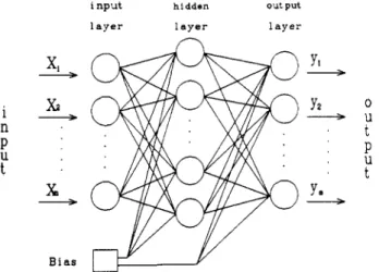
Figure 1. Multilayered feedforward neural network.

imal requirement of a diagnostic system for any practical application.

The purpose of this work is to provide a self-learning feature to the qualitative/quantitative model-based diagnostic system. The self-learning procedure is based on reinforcement learning of the neural network (Barto et al.,

1983). Comparisons will be made between the qualitative/quantitative model-based system from reinforcement learning and the well-celebrated quantitative model-based system, artificial neural network using backpropagation learning. A CSTR example will be used to illustrate the model building, self-learning, and performance of these two systems. This paper is organized as follows. ANN with backpropagation learning and reinforcement learning is introduced in section 2. Section 3 describes how to add the self-learning feature to the qualitative/quantitative model. Model-based diagnostic systems are given in section 4. A CSTR example is used to illustrate the charac-

teristics of these two systems in section 5, followed by the Conclusion in section 6.

2. Artificial Neural Network

An artificial neural network (ANN) is trained to produce a desired output by adjusting the weights on the connec- tions between nodes according to some prespecified criteria. Generally, three types of learning procedures exist: (1) supervised learning, (2) unsupervised learning, and (3) reinforcement learning. The relevant two, the supervised and reinforcement learning, are described here.

2.1. Supervised Learning. ANN with backpropagation learning is a typical example of supervised learning. In the supervised learning, an external target output vector is required for each input vector. A common procedure

is to adjust the values of the weights such that the s u m of the squares of the deviations between the target value and each actual output is minimized (Rumelhart and McClelland, 1986; Lippmann, 1987). Figure 1 shows a multilayer feedforward neural network architecture. The circles (nodes) represent the processing elements in different layers: input, hidden, and output layers. Each input

unit is connected to each hidden unit and each hidden unit is also connected to each output unit. Each hidden and output unit is also connected to a bias. The bias with the value of 1 is used in this work. Each connection has a weight associated with it. For the input layer, an input value is straightly forwarded to the next layer. The hidden and output units carry out two calculations. Firstly, a weighted sum of the inputs is taken (e.g., ajj), and then the output is calculated using a nondecreasing and differen- tiable transfer function f(aj) (Figure 2). Usually the

Figure 2. Processing element (neuron).

I

-10 -5 0 5 10

a j

Figure 3. Processing element output transfer function.

transfer function f ( a j ) is a sigmoid logistic function as shown in Figure 3.

(1)

Typically, the learning rule for adjusting the weights is the generalized delta rule (GDR) (Rumelhart and McClelland, 1986). It uses the gradient-descent method to minimize the objective function E (or the mean square error):

(2)

where

M

is the number of training patterns presented to the input layer and

N

is the number of units in the output layer, dr represents the target output value of the ith output element given the mth pattern, while yr is the actual output of the ith unit.

For a given pattern, the weight is adjusted according to GDR as the following:

(3)

where wij(t+l) denotes the weight of the connection between the ith element of the lower layer and the jth element of the upper layer in the (t

+

11th learning iteration. The weight change Awij(t) in eq 3 is calculated according to

(4)

where t and /3 are the learning rate and momentum con-

stant; xi is the output value of the ith element in the lower layer. The momentum term B prevents divergent oscilla- tion and makes the convergence more rapidly. The error term of the jth element Sj in eq 4 is determined as follows. If the subscript j denotes the output layer, then

(5) f(aj) = 1/(1

+

e-"))

l M N 2 m = l i = l

E = -

c

E(dY

- YT)2

wij(t+l) = wij(t)

+

Awij(t)

Awij(t) = $ j ~ i

+

/3Awij(t-1)

sj

= (dj - Yj)fj'z(wijxi

+

ej)

1

and if j denotes the hidden layer, we have

6 j = fj'c(wijxi

+

8 j ) E 6 k W j k (6)

where fj' is the derivative of the jth transfer function as described previously, 0, is the bias of the connection in the jth element, and k is the upper layer element of the j t h

element.

(4)

reinforcement ( r )

Ind. Eng. Chem. Res., Vol. 31,

No.

8, 1992 1939

( A ) m

Y

0 A B / A A ( s t a t e feedback) Figure 4. “Boxed’ system.

network has the following training steps: patterns.

According to the generalized delta rule (GDR), the

1. Initialize the weights randomly and specify the bias.

2. Specify the input patterns and the target output 3. Calculate the actual output pattern.

4. Adjust the weights by GDR.

5. Check the convergence criterion; if it is satisfied then go to step 6, otherwise go back to step 3.

6. Stop.

2.2. Reinforcement Learning. Another learning al-

gorithm of

ANN

is the reinforcement learning (Barto et al., 1983). Typical applications of reinforcement learning are in control problems (e.g., fuzzy control of a cart-pole system;

Lee,

1991). It uses a neuronlike element to solve the specified problem. Usually this element is called associative search element (ASE). One important difference between the supervised learning and the reinforcement learning is that the supervised learning must have a target value to correct (e.g., minimizing) the error between the actual output value and the target value. If the environ- ment is unable to provide the appropriate response for a desired performance, then the ASE must discover what response can lead to an improvement in the performance. It employs a trial and error procedure to search for appropriate action and f i d e an indication of the performance. The appropriateness of such action can be judged from the performance, measure. If the value of output units action is bad (does not lead to improvement), then it adjusts the weight by some strategy to keep getting good results. This is

similar

to a child learning to taste candy by trial and error until he fiids what he likes.

In the “Boxes” system (Barto et al., 1983), the ASE is employed in a self-learning controller to control a &-pole system. The element has a reinforcement input pathway, n pathways for nonreinforcement input signals, and a single output pathway as shown in Figure 4. The decoder divides the continuous output signal into discrete states. The element’s output y ( t ) is determined from the input vedor X(t)

=

[ q ( t ) , x&),

...,

x,(t)] as follows:

(7)

where f is the following threshold function (a step func- tion):

y ( t ) = flCwi(t)xi(t)

+

noise]

i-1

A x ) =

I

+1 i f x z 0

-1 i f x c O

The weights wi)s are changed according to

wi(t+l) = wi(t)

+

ar(t) ei(t) (9)

ei(t+l) = 6eiW

+

(1 - 6)y(t) x i ( t ) (10)

where a = learning rate, 6 = trace decay ratio, r(t) = reinforcement signal at time t, ei(t) = eligibility at time t of input pathway i, and x i ( t ) = input vector at time t. Spe-

A

+ B

7‘1

‘ I

Y

A

9 B

Figure 5. Membership functions for (A) qualitative model and (B) qualitative/quantitative model.

cifically, the Boxes system divides the system inputs into many substrates (input pathways) by the decoder. The system performance is judged according to the inputs. If the performance is bad, then the system gives a reinforcement signal r. Whenever certain conditions hold for the ith input xi, then this pathway becomes eligible to have

its weight modified. In the Boxes system, the input x i

triggers the eligibility trace whenever the box i is entered. According to r and the eligibility, a better performance is sought by changing the output (action) via the adjustment of the corresponding weight.

3. A Self-Learning Qualitative/Quantitative Model

3.1. Qualitative/Quantitative Model. In qualitative reasoning, the diagnostic resolution is limited by the strictly qualitative knowledge. Yu and Lee (1991) integrated the semiquantitative knowledge into a qualitative model using fuzzy set theory. The shape of the membership function represents the semiquantitative information between process variables. Consider a simple qualitative model: the signed directed graph (SDG), e.g., A L B . The binary relation between A and B can be de- scribed by the ratio

m/AA

taking the value from O+ to infiiity. In terms of the qualitative/quantitative model,

the membership function ~ l g ~ ( h B / b A ) takes the value of

1 for all positive M/&4 as shown in Figure 5A. If some semiquantitative information is known, e.g., the steady-

state gain between A and B falls between 2 and 4, we can modify the membership function accordingly (Figure 5B). However, the construction of the semiquantitative knowledge requires a great deal of engineering effort, even when all process data are available. Furthermore, the semiquantitative knowledge needs to be modified as we change the operating conditions. One important advantage of the quaiitative/quantitative model is that the qualitative

part of the model (the structure) remains the same under

almost all possible operating conditions. Therefore, when the operating condition changes, all one has to do is to modify the semiquantitative part of the proce-sa knowledge.

3.2. Self-Learning Feature via ASE. Reinforcement learning is employed to acquire the semiquantitative knowledge automatically. The basic idea is shown is Figure 6. For a given fault origin, we can find measurement patterns from process simulation or past events. The measurement patterns are fed into the qualitative/quan-

(5)

1940 Ind. Eng. Chem. Res., Vol. 31,

No.

8, 1992 Neural Updating me a s UT ernent

I

Mode1 d i a g n o s i s patterns r e s u l t s \I I

Fault

Origin

Figure 6. Schematic representation of a self-learning procees for the

qualitative/quantitative model-based diagnosis system.

'B

A B / A A

A

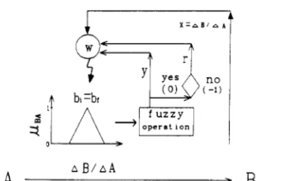
Figure 7. Schematic representation of reinforcement learning via information on qualitative/quantitative model.

titative model. If the fault is not correctly identified, the reinforcement learning is activated and the measurements and the diagnostic results are fed to the corresponding ASE. Subsequently, the shape and location of the membership function is changed until a satisfadory diagnostic result is found ( F i e 6). That is, the model learns from the measurement pattern repeatedly until good performance (correct diagnosis) is achieved. In the meantime, the membership function in the model (the semiquantitative knowledge) is adjusted to ensure good performance. Let

us take a single branch between nodes A and B and ita corresponding ASE as an example (Figure 7). Initially, the membership function is located according to the measurement

AB/AA.

This value corresponds to the full membership, i.e., p B A ( A B / A A ) = 1, and the membership decreases linearly to zero for 120% deviations in

ABIAA.

If another set of measurement pattern is available and the result of the fuzzy operation is not satisfactory, e.g.,

p B A ( A B / A A ) # 1, then the system responds with a rein-

forcement signal r = 1. This indicates the location and shape of the membership function is incorrect (Figure 7). Therefore, the ASE reshapes the membership function

1 s t learning

A B / A A

A z

Figure 8. Learning steps for the ASE.

according to

hB/AA

and p s ~ ( u / A A ) until a good performance p g A ( A B / A A ) = 1 is achieved. The membership function is relocated according to the weight change Aw (Aw = w ( t + l ) - w(t)). In this work, the weight w is changed according to

w ( t + l ) = w(t)

+

a r ( t ) e ( t ) (11)

e(t+l) = 6e(t)

+

(1

-

6)(1

-

y ( t ) ) x ( t ) (12) where CY = learning rate, 6 = trace decay ratio, r ( t ) = re-

inforcement signal at time t, e(t) = eligibility at time t, and

y ( t ) = the result of fuzzy operation at time t. The ASE

adjusts the location and shape of the membership function in the following way:

I b l i f x > b f

I

-IAwl i f b i > x

A x ) = 0 i f b i < x < b f (13)

where bi and bf are the initial and final valuea of the process measurements satisfying y = 1. That is, bi and bf corre- spond to the upper left and right comers of the trapezoid shaped membership function.

As

shown in Figure 7, the following information (1)

proms measurement xi (or ABIAA), (2) the result of fuzzy

operation y (or p B A ( A B / A A ) ) , and (3) reinforcement signal r are utilized to change the weight of ASE. Then, the correct location and shape of the membership function is determined by the weight change. The triangular mem- bership function (Figure 7) is initialized as the process information is available.

As

additiod proms information is available, the self-learning process does the following. 1. It gives appropriate output Cy = p B A ( A B / A A ) ) according to the membership function.

2. When a failure signal (Le., y # 1) is received, it adjusts the weight according to eqs 11 and 12. The membership function is reshaped according to eq 13 when Aw is available.

3. Repeat steps 1 and 2 until the correct diagnosis Cy = 1) is achieved.

Therefore, the membership function is modified itera- tively until the correct diagnosis, p ( A B / A A ) = 1, is achieved m shown in Figure 8. Typically, it

takes

less then 10 iterations to converge.

It is clear that the ability of the ASE goes beyond this type of application. In the Boxes system (Barto et al.,

1983), it searches for appropriate control action as the state feedback becornea available. The control system emits the control action and the performance is evaluated. When a failure occurs, the reinforcement learning is made and another action is taken. Since the result of each learning step is checked on-line, the speed of convergence (to a successful leaming) is critical for the control applications. In diagnosis, the performance after each learning step can

easily be evaluated (to check whether y = 1 or not). Therefore, the speed of convergence is less critical. How-

ever, it differs from the box system in that the ASE rec- ognizes that the reinforcement learning is to include ad- ditional process information as another valid set of input.

2 n d learning , , , I h h learning A b i b i A b i bf * E A B / A A

B

A r B A A B / A A

(6)

Ind. Eng. Chem. Res., Vol. 31, No. 8, 1992 1941

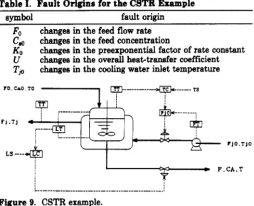
Table I. Fault Origins for the CSTR Example

SWllbol fault origin

Fo

C, KO U

T p

changes in the feed flow rate changes in the feed concentration

changes in the preexponential factor of rate constant changes in the overall heattransfer coefficient changes in the cooling water inlet temperature

r0 CAO TO D 1s I I J TIO.Tl0 I A

y

C F.CA.T I I I L I Figure 9. CSTR example.

Therefore, the staircase-like transfer function ( f ( x ) in eq

13) is used instead of the step function (Barto et al., 1983). Following this procedure, the self-learning qualitative/ quantitative model remembers semiquantiative informa- tion at different operating conditions.

In the qualitative/quantitative fault model, there is an

ASE

associated with each branch for every fault origin. It provides the self-learning feature to the fault model such that the appropriate membership function is constructed to give correct the diagnosis (response) at different operating conditions.

4. Fault Diagnosis Systems

Two on-line diagnosis systems are investigated in this work. Both systems are associated with an artificial neural network (ANN), in some sense, e.g., either in the model

structure or in the self-learning step. One system is the

ANN with backpropagation learning which currently is the

prototype of quantitative model-based diagnosis system (Watanabe et al., 1989; Venkatasubramanian et al., 1990, Ungar et al., 1990). This system can be viewed as a quantitative model which has the model structure of ANN. The other system utilizes the learning ability of the neural network to find the semiquantitative information. Spe- cifically, it is a qualitative/quantitative model-based sys-

tem with self-learning capability. A CSTR example

(Figure 9) is employed to show the similarity and difference between these two systems. Before building any diagnosis system, the fault origins and process measurements have to be identifed. For the CSTR example, the fault origins are listed in Table I. These faults include load changes (Fo, Ca0, and Tj0) and performance deterioration

(U

and

KO).

The process measurements are temperatures, flow rates, and control signals as shown in Table 11.

4.1.

A N N

with Backpropagation Learning. The inpub and outputs of the ANN with backpropagation

learning are process measurements and fault origins, respectively. Once the process measurementa are determined (Table 11), the inputs to the ANN are obtained from the plant data or the results of computer simulations. In this

0.24 0.015 1.W

Table 11. On-Line Measurements for the CSTR

Symbol measured variable

T reactor temperature

cooling water outlet temperature cooling water flow rate

Tj

temperature controller output

Fj

Tc

Fje cooling water flow controller output

Lc reactor level controller output

Table 111. ANN Target Output Pattern

fault F0- 1.0 FO+ 0.0 Go- 0.0

c,+

0.0 KO- 0.0 F0- 0.0 0.0

2;

0.0 normal 0.0

target output pattern 0.0 0.0 0.0 0.0 0.0 0.0 1.0 0.0 0.0 0.0 0.0 0.0 0.0 1.0 0.0 0.0 0.0 0.0 0.0 0.0 1.0 0.0 0.0 0.0 0.0 0.0 0.0 1.0 0.0 0.0 0.0 0.0 0.0 0.0 1.0 0.0 0.0 0.0 0.0 0.0 0.0 1.0 0.0 0.0 0.0 0.0 0.0 0.0 0.0 0.0 0.0 0.0 0.0 0.0 0.0 0.0 0.0 0.0 0.0 0.0 0.0 1.0 0.0

work the quasi-steady-state results of the process simulator are employed to train the network. Typically, these variables are expressed in a dimensionless form.

(14)

The target output patterns are determined from the fault

origins

with

positive and/or negative deviations (Table m).

In this work, there are five inputs and eight outputs in the

ANN. In Table 111, the value of "1" stands for a faulty

state and "0" stands for normal operation. With input and output patterns available, the GDR is employed to su- pervise the learning of the network until the actual output patterns are close to the target output patterns within a threshold value.

Before the training procedure begins, several importance parameters, such as the number of elements in each layer and learning constants, have to be determined.

As

noted earlier, the number of elements in the input and output layers is chosen according to the measured variables and fault origins. However, there is no exact method to de- termine the number of elements in the hidden layer and learning constants. Generally, adquate values of these parameters are determined by trial and error (Watanabe et al., 1989; Venkatasubramanian et al., 1990).

4.2. Qualitative/Quantitative Model with Rein- forcement Learning. The qualitative part of the model

has the structure of a signed directed graph (SDG) which describes the causal effect between process variables. All the nodes, except the initial node (the fault origin), in a SDG are process measurements (Figure 10). The quan- titative part of the model is formed using the membership function of fuzzy set theory as described in detail by Yu and Lee (1991). In this work, the semiquantitative knowledge is constructed via reinforcement learning. For the diagnostic system, the qualitative/quantitative models are constructed for both the steady state and the transient

state. The dynamic responses of a faulty state are used to train the model for the diagnosis during the transient. When the changes of the process variables are leas than

measured x

-

nominal x nominal x x =

A T C A F I C / A T C A F I / A F I C A T j I A F j

C A O

-

T C

-

F j c

-

F j

_{T j}

(7)

1942 Ind. Eng. Chem. Res., Vol. 31, No. 8, 1992

- _t _t - -

Fa

-

L c T c

-

F i c

-

F I

-

T I

t

T l a Tc

-

F i c

-

Fi

Figure 11. Qualitative models (SDG) for all the fault origins.

5% between sampling instances, the steady state (or quasi steady state) is recognized and the corresponding process measurements are employed to train the model for the diagnosis at steady state. Therefore, these two qualitative/quantitative models handle the transient and steady-state responses separately.

The rule writing for the qualitative/quantitative model is similar to that of the qualitative model (Chang and Yu, 1990). That is, the degree of consistency for each fault propagation pathway is checked (Yu and Lee, 1991). For the CSTR example (Figure 91, the self-learned system results in the qualitative/quantitative model (Figure 10) for a negative deviation in Cap The membership functions in Figure 10 are obtained via reinforcement learning using

several sets of quasi-steady-state information (-10, -30 and

-60% deviations in Cap The rule can be written as

P C ~ - = min [cLT,(ATC), pF,,T,(Ujc/ATc),

where pc - is the truth value for Cao going through a

negative %ange, the “min” operator taking the smallest value in the bracket. Here, ~T,(AT,J, ~ F ~ , ( M ~ , / A T , J , etc. are the degree of consistency for each branch in Figure 10. Similarly, rules can also be written for the positive deviations in Cao and other fault origins.

5. Applications

A CSTR example (Chang and Yu, 1990; Yu and Lee, 1991) is used to illustrate the performance of the qualitative/quantitative model with reinforcement learning. The proposed approach is compared to the ANN diagnostic system with backpropagation learning.

5.1. Process. In this example, an irreversible and

exothermic reaction is carried out in a perfectly mixed CSTR as shown Figure 9. Parameter values are taken from Luyben (1990). Eight faulty states with both the negative and positive deviations (Table I) are to be diagnosed. Table I1 shows the measured variables in this study. Basically, these measurements can be obtained with little difficulty. Notice that the concentration of the reactant A in the reactor, C,, is not included. The consideration is a practical one: on-line composition measurements often are not available in reaction units. This example poses a difficult diagnosis problem. If only qualitative process measurements are available, the faults Cao,

KO,

and

U

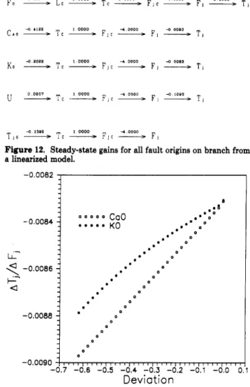
(the changes in feed concentration, rate constant, and overall heat-transfer coefficient) are indistinguishable as shown in the SDG’s of the fault origins (Figure 11). However, if quantitative process measurements are available, only two faults Cao and

KO

are not distinguishable (Figure 12). Figure 12 shows that the steady-state gains between measured variables which are derived from the linearized

p F S ; , ( U j

/

Mjc) c(T,F, (ATj/ Uj)

1

(15) C l o

-

4 4122 Tc

-

I 0000 F , c

-

4 0000 F i

-

-0 0083 T i -3 ZOZZ I 0000 4 0000 -0 0083 K o ---e- Tc

-

F J c

-

F i

-

T i 4 13QP 1 0000 4 0000 T i a ----+ T c

-

F i c _jl F i

Figure 12. Steady-state gains for all fault origins on branch from a linearized model.

rn

-0.0082 -0.0084 - LL- &- a

e

-0.0086 0 0 -0.0090

j

I, ,IJ IIII, ,III~II1 1), II,~, ,, I), ,,,, ,,I 1_ 0 -0.7 -0.6 -0.5 -0.4 -0.: -0.2 -0.1 -0.0 0 Deviation I

Figure 13. Steady-state gains for the branch *Fj

-

T,” for different degrees of negative deviations in CaO and KO.

process model. Therefore, from the linear analysis, fault in Cao and

KO

cannot be separated. However, for a range of deviations in

C

,

and

KO,

the steady-state gains between the nodes Fj-Tj are not quite the same as shown in Figure 13. That is, it is possible to distinguish these two faults from a nonlinear analysis. It should be pointed out that the magnitudes of the faults of interest are between 10% and 60%. In this work, the sampling time for the diagnostic system is 3 min. That is, the process measurements are sampled every 3 min and the diagnosis is made right after. Therefore, the diagnosis results can be shown on the CRT of the process control computer as the “diagnosis”

trend.

5.2.

ANN

Diagnostic Systems. Two ANN’s with

backpropagation learning are constructed and tested for this CSTR example. These two ANN’s differ in the numbers of input patterns and the structure (the numbers of hidden layers).

In the first ANN, two input patterns, 10% and 30% deviations in the fault origins, are employed for each fault origin. The process measurements are obtained from process simulation when the responses approach steady- state (e.g., at 3.5 h after the fault initiates). The fault origins and target output patterns are shown in Table 111. The input variables are the on-line measurements including

L,,

T,,

T,

F,,

and

Tj

(Table 11). After a period of trial and error, a three-layered neural network is chosen. The numbers of the elements in the input, hidden, and output layers are 5, 10, and 8, respectively (Figure 14). This neural network is called ANN(1) hereafter. The

(8)

Ind. Eng. Chem. Res., Vol. 31, No. 8, 1992 1943 Tjo- 0.0 0 U n I t

E

e

1 t '

-

7 B i a s W

Figure 14. ANN diagnostic system (A"(1)).

measurements far input pattern( Cc,Tc,T,Fj,Tj )

Fo-

4

c

0 . 0 1 I ~I

,

I

1-Iteration number

Figure 15. Convergence of the objective function for ANN(1).

learning rate 9 = 0.6 and momentum term /3 = 0.9 are used in ANN(1). It takes approximately 13000 iterations to converge to the criterion E C 0.08. The response of learning is shown in Figure 15.

Once the ANN(1) is constructed and the training is successful (satisfying the convergence criterion), the diagnostic system is

tested

on-line. For the trained patterns, e.g., -30% deviation in Cao, A"(1) gives a perfect result. Figure 16 shows that ANN(1) identifies the fault origin

(Cao-) correctly 1 h after the fault starts. Furthermore, there is no spurious solution in this case. That is, ANN(1) does a superb job in identifying the fault origin for the trained pattern. Note that only steady-state information is used in the training step. Unfortunately, ANN(I) gives an erroneous solution (fails to identify the true fault origin) as interpolation and/or extrapolation between input patterns is required (Figures 17 and 18). Figure 17 shows that when Cao goes through a range of negative deviation

(-10% to 4%),

A " ( D

miseee the true fault origin

(Ca-)

for ACao between -12% and -25%. In this case, ANN(1)

finds the fault origin KO- instead (Hau, 1991). The results shown here reveal a serious problem associated with A"(1): the only solution given by A"(1) is erroneous. Similar results can also be found for a range of deviations

in

KO

(Figure 18). Again, ANN(I) gives erroneous solutions

(finds Cao- instead) for two ranges of AKo as shown in Figure 18.

In order to improve the performance of ANN(I), an attempt is made by including another input pattern (60% deviation in the fault origin) to train the ANN model.

...

*

....

...e

...

KO-

0.0 1

-

0.0 t 1

Figure 16. Diagnosis results of ANN(1) for a 30% negative devia- tion in Ca0 (a trained input pattern).

Figure 17. Diagnosis results of ANN(1) for a range of negative deviations in C,, (-10% to -60%).

However, the three-layered neural network (Figure 14) fails

to converge. A four-layered neural network is teated. After some trials and errors, the ANN with the numbers of elements of 5,15,15, and 8 in the input layer, hidden layer 1, hidden layer 2, and the output layer is chosen. The learning rate q and momentum term are 0.1 and 0.9, respectively. This neural network is called A"(I1) hereafter. The differences between A"(1) and A"(I1) are ANN(I1) is a four-layered neural network and three input patterns for each fault origin are employed in ANN(I1). Upon diagnwis, ANN(II) elso performs perfectly for the

(9)

1944 Ind. Eng. Chem. Res., Vol. 31, No. 8,1992

, r

Figure 20. Diagnosis results of ANN(I1) for a range of negative deviations in KO (-10% to -60%).

steady-state qualitative/quantitative model can be found

via reinforcement learning. The proceas measurements (Tc, F,,, F,, and T,) at quasi steady state (1.5 and 4 h after the occurrence of the fault) are recorded and converted to steady-state gains for the training of the corresponding branches. Therefore, there are six data points for a single branch. For the branch between F, and TI (Figure

lo),

the gains range from -0.0067 to -0.0087. Initially, one has no a priori knowledge about the location of the membership function. When the information comes in (ATJAF, = -0.0067), a triangular-shaped membership function is formed with the apex located at -0.0067 and it decreases linearly to zero for &30% deviations from the apex ( p

becomes 0 at -0.0045 and -0.0089). When the second set of data comes in (AT,/AF, = -0.0087), an unsatisfactory diagnosis result is obtained, Le., p T , ~ (ATJAF,)

-

0, and the reinforcement signal is activated ( r = 1). The ASE adjusts the membership function in the following way (Figure 7): (1) calculating e(t+l) from eq 12, (2) finding Aw using eq 11, and (3) changing the membership function according to eq 13 (initially b, = bf = -0.0067). These three steps are repeated until a satisfactory diagnosis results (i.e., pTF,(-0.0087) = 1). In this example, it takes two iterations to converge and the resulting semiquantitative model is shown in Figure 10 (the F,-TI branch). Since the other four gains falls between -0.0067 and -0.0087, satisfactory diagnostic results are produced and the ASE is not activated. This procedure is repeated for all branches with

all fault origins. In this work, the learning rate of 1 and the trace decay ratio of 0.9 are used throughout. A typical

qualitative/quantitative model constructed from reinforcement learning is similar to the one shown in Figure

10.

In the diagnosis phase, the diagnostic system is tested against each fault origin with a range of deviations. The procedure for fault diagnosis is exactly the same as that of Yu and Lee (1991). Unlike the ANN diagnostic systems,

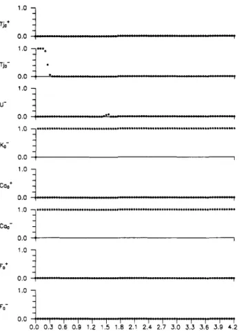
e.g., ANN(1) and ANN(It), the proposed diagnostic system does not give erroneous solutions (Figure 21). Figure 21

shows that the qualitative/quantitative model-based diagnostic finds the true fault origin for a range of negative deviation (-10% to -60%) in Cap However, it results in spurious solutions as shown in a -20% deviation of CaO

(Figure 22) or a -20% deviation of KO (Figure 23). In both cases, it finds Cao- and KO- as the fault origins. Despite

Figure 18. Diagnosis results of ANN(1) for a range of negative deviations in KO (-10% to -60%).

Figure 19. Diagnosis results of ANN(I1) for a range of negative deviations in Cd (-10% to -60%).

1991)). Unfortunately, ANN(I1) also gives erroneous solutions for the ranges of deviations in Ca0 and

KO

(Figures 19 and 20). Furthermore, for the fault origin CaO-, diagnostic results simply deteriorate as shown in Figures 17

and 19. Apparently, little improvement is achieved by including one more input pattern and one more hidden layer. The characteristics of A"(1) or ANN(I1) shown here certainly limits the applicability of ANN in any practical situation for this type of process. Note that the results shown here do not imply that backpropagation ANN is not suitable for fault diagnosis in all cases. The CSTR example poses a very difficult diagnosis problem

as pointed out earlier.

5.3. Qualitative/Quantitative Diagnostic Systems.

The qualitative part of the fault model is constructed fmt followed by the self-learning of the semiquantitative knowledge. In the self-learning phase,

lo%,

30%, and

60% deviations in each fault origin are used to shape the semiquantitative process knowledge using ASE. Let us consider the case of Cao going through negative changes

(10)

Ind. Eng. Chem. Res., Vol. 31, No. 8,1992 1946 Tja* ''O

1

I 0.0 Tjo- - U' 0.0

Figure 21. Diagnosis results for the qualitative/quantitative model for a range of negative deviations in ,C (-10% to -60%).

KO- - 0.0 1 .o Th* 0.0 1 .o Tjo- 0.0 1 .o U- 0.0 1 .o KO- 0.0 1 .o Can' 0.0 1 .o C%- 0.0 1 .o Fa' 0.0 1 .o Fa' 0.0 I

I-

Coo- 0.0 I ~

...

"..".

...

....

- l-

."..

i

....

T

-.

_- 1 1 1 1 0.0 0.3 0.6 0.9 1.12 1.k 1.8 2.'1 2.; 2.5 3.b 3.5 3.6 3.b 4.2 lime (hr)

Figure 22. Diagnosis results for the qualitative/quantitive model

for a 20% negative deviation in Caw

the possibility of giving spurious solutions, the qualitative/quantitative diagnostic system shows a very desirable characteristic: it does not give erroneous interpretations. The reason is that the membership function-based qualitative/quantitative model adapts to new (additional) information by including it (instead of changing to a new crisp point as quantitative models do). This clearly shows the flexibility of the qualitative/quantitative model (as

opposed to the rigidity of quantitative models). In sum- mary, the qualitative/quantitative model-based diagnosis

1- ..7 ...

-...

, 0.0 0.0 0.3 0.6 0.9 1.2 1.5 1.8 2.1 2.4 2.7 3.0 3.3 3.6 3.9 4 . 2 Time (hr) Figure 23. Diagnosis results for the qualitative/quantitative model for a 20% negative deviation in KO.

system has the advantage over the strictly quantitative model-based system (e.g., ANN(1) and ANN(II)), since it did not produce erroneous solutions. It also has the advantage over the strictly qualitative model-based system (e.g., SDG) for producing less spurious solutions. Fur- thermore, the semiquantitative information is self-learned via the ASE which requires little engineering effort.

5.4. Discussion. Despite the fact that both diagnostic systems have the "learning" feature, the performance between the two is quite different. The ANN'S (ANN(1) and ANN(I1)) try to learn to reproduce the trained input, patterns. However, the backpropagation learning of ANN

ignores an engineering fact that the gains between T,-Fj are almost the same for the fault origins Cao and

KO.

Without taking this fact into consideration, GDR simply tries to converge to the target output patterns by assigning

one range of ATj/Mj to Cao and another range of ATj/AFj to

KO

(e.g., Figure 13) according to the input patterns supplied. Therefore, the ANN diagnostic system does not catch the global view; e.g., ATj/AFj for both fault origins can take any possible value between 4.0083 and 4.0088.

This, subsequently, leads to erroneous solutions as shown

in the diagnostic results.

The self-learning feature of the qualitative/quantitative model, on the other hand, is confined to the semiquantitative part of the process knowledge. That is, we keep the structure of the model unchanged and modify the more rigid quantitative information when needed. Furthermore, the reinforcement learning modifies the membership function by including the new process data instead of adapting to the new information. "Learning" under theae guidelines is not likely to give erroneous solutions when we interpolate between the trained patterns. The diagnostic results also confirm this.

(11)

1946 Ind. Eng. Chem. Res., Vol. 31, No. 8, 1992

It should be emphasized that the CSTR example studied

poses a quite difficult diagnosis problem. This difficulty

results from the selection of the process measurements and

faults to be diagnosed. For example, if

C,

is measurable,

all the fault origins can be correctly identified with only

qualitative values of process measurements (Hsu, 1991).

This implies that, in many occasions, the difficulty in

diagnosis arises from the selected measurements, not from

the process itself. Therefore, selection of the appropriate

measurements for fault diagnosis can simplify the effort

in fault diagnosis.

6. Conclusion

A self-learning feature is proposed for the qualita-

tive/quantitative model-based diagnostic system. Based

on the reinforcement learning of neural network, a single

neuron (ASE) is used to shape the semiquantitative part

of the process knowledge. This provides the self-learning

ability to a diagnostic system in a transparent manner.

Comparisons are made between the qualitative/quanti-

tative model with reinforcement learning and the ANN

with backpropagation learning. Simulation resulta show

that the proposed self-learning diagnostic system is not

only transparent in analyses but superior in performance

(as far as the completeness is concerned). More impor-

tantly, the self-learning feature makes the qualitative/ quantitative model-based diagnostic system attractive in

practical applications, since i t requires much less engi-

neering effort.

Acknowledgment

of the ROC under Grant NSC 81-0414-P-011-04-B.

This work is supported by the National Science Council

Nomenclature

ANN = artificial neural network

ASE = associative search element

bi = initial value in the membership function (the upper left corner of the trapezoid)

bf = fiial value in the membership function (the upper right

corner of the trapezoid)

C, = concentration of reactant A

Ca0 = feed concentration of reactant A

di = desired output value

e = eligibility

E = objective function

f ( - ) = transfer function in the neural network

f’(.) = derivative off(.)

Fo = feed flow rate

Fj = cooling water flow rate

Fj, = cooling water flow controller output GDR = generalized delta rule

KO = preexponential factor of the rate constant

L, = reactor level control output

min (.) = minimum value of (-)

r = reinforcement

SDG = signed directed graph

T = reactor temperature

T, = temperature controller output

Tjo = cooling water inlet temperature

t

+

1 = ( t

+

1)th iteration

U = overall heat-transfer coefficient

w = weight in ASE

wi = weight of input pathway in the Boxes system

wi, = weight between the ith element of the input layer and

Aw = weight change in ASE

Awi, = change of weight between iterations

x = input to ASE

the j t h element of the upper layer

z i = ith input of backpropagation ANN

y = output of ASE

yi = ith output of backpropagation ANN

Greek Symbols

a = learning rate in ASE

@ = momentum term in backpropagation ANN

6 = trace decay rate in ASE

6j = error term in backpropagation ANN

tl = learning rate in backpropagation ANN

0, = bias in backpropagation ANN

pA = membership function of A

Literature Cited

Barto, A. G.; Sutton, R. S.; Anderson, C. W. Neuronlike Adaptive Elements That Can Solve Difficult Control Problems. ZEEE

Trans. Syst., Man Cybern. 1983, SMC-13,834-847.

Chang, C. C.; Yu, C. C. On-Line Faults Diagnosis Using Signed

Directed Graph. Znd. Eng. Chem. Res. 1990,29, 1290-1299.

Cheung, J. T. Y.; Stephanopoulos, G. Representation of Procese

Trends-I A Formal Representation Framework. Comput. Chem.

Eng. 1990a, 14, 495-510.

Cheung, J. T. Y.; Stephanopoulos, G. Representation of Process Trends-11 The Problem of Scale and Qualitative Scaling. Com-

put. Chem. Eng. 1990b, 14, 511-539.

Frank, P. M. Fault Diagnosis in Dyanmic Systems Using Analytical

and Knowledge-Based Redundancy-A Survey and Some New

Results. Automatica 1990,26,459-474.

Himmeblau, D. M. Fault Diagnosis and Detection in Chemical and

Petrochemical Processes; Elsevier: Amsterdam, 1978; p 1.

Hsu, Y. Y. Automatic Fault Diagnosis Systems: Associative Rein-

forcement Learning. M.S. Thesis, National Taiwan Institute of

Technology, Taipei, 1991 (in Chinese).

Isermann, R. Process Fault Detection Based on Modeling and Es-

timation Method-A Survey. Automatica 1984,20,387-404.

Kramer, M. A.; Palowitch, B. L., Jr. A Rule-Based Approach Diag- nosis Using the Signed Directed Graph. AIChE J. 1987, 33, Kuipers, B. The Qualitative Calculus is Sound but Incomplete: A

Reply to Peter Stms. Artif. Zntell. Eng. 1988, 3, 170-173.

Lee, C. C. A Self-Learning Rule-Based Controller Employing Ap- proximate Reasoning and Neural Net Concepts. Znt. J. Intell.

Syst. 1991, 6, 71-93.

Lippmann, R. P. An Introduction to Computing Neural Nets. ZEEE,

ASSP Mag. 1987, April, 4-22.

Luyben, W. L. Process Modeling, Simulation and Control for

Chemical Engineers, 2nd ed.; McGraw-Hilk New York, NY, 1990;

p 124.

Petti, T. F.; Klein, J.; Dhurjati, P. S. Diagnostic Model Processor:

Using Deep Knowledge for Fault Diagnosis. AIChE J. 1990,36,

565-575.

Pramd, P. R.; Davis, J. F. A Framework for Implementing On-Line

Diagnostic Advisory Systems in Continuous Procese Operations.

AIChE Annual Meeting, Nov 17-22,1991, Los Angeles.

Rengaswamy, R.; Venkataaubramanian, V. An Integrated Frame-

work for Process Monitoring, Diagnosis, and Control Using

Knowledge-Based Systems and Neural Network. IFAC Sympo-

sium on On-Line Fault Detection and Supervision in Chemical

Process Industries, April 22-24, 1992, Newark, DE.

Rumelhart, D. E.; McClelland, J. L., MS. Parallel Distributed Pro- cessing; MIT Press: Cambridge, MA, 1986; p 324.

Ungar, L. H.; Powell, B. A.; Kamens, S. N. Adaptive Networka for

Fault Diagnosis and Process Control. Comput. Chem. Eng. 1990,

14, 561-572.

Venkataaubramanian, V.; Vaidyanathan, R.; Yamamoto, Y. Procese

Fault Detection and Diagnosis Using Neural Networks-I.

Steady-State Process. Comput. Chem. Eng. 1990,14, 699-712.

Watanabe, K.; Matauura, I.; Abe, M.; Kubota, M.; Himmelblau, D. M. Incipient Fault Diagnosb of Chemical Proceesee via Artificial

Neural Networks. AZChE J. 1989,36, 1803-1812.

Willsky, A. S. A Survey of Design Methoda for Failure Detection in

Dynamic Systems. Automatica 1976,12,601-611.

Yu, C. C.; Lee, C. Fault Dwosis Based on Qualitative/Quantitative

Process Knowledge. AZChE J. 1991,37,617-628.

Received for review July 25, 1991

Revised manuscript received December 12, 1991

Accepted March 23, 1992 1067-1087.