Economic growth, national competitiveness, and stock retrun

全文

(1)國立政治大學財務管理研究所碩士論文. Economic Growth, National Competitiveness and Stock Return. 立. 政治大. ‧. ‧ 國. 學 y. Nat. Advisor:. n. al. er. io. sit. Ph.D. Edward H. Chow. Ch. engchi. i n U. v. Author : Yen-Wen Wang. June 2012.

(2) 謝誌二年的政大碩士生涯轉眼就結束了，一路走來所有的酸甜苦辣箇中滋味只有自己最了解，一切的汗水與努力都將化為最甜美的果實。感謝讓我結交到一群共同學習，共同成長的好朋友，永遠記得在研究室的埋首論文撰寫，同學間的砥礪切磋以及在教室上課的點點滴滴，認識你們是我這輩子最美好的事物之一。感謝指導我的指導老師：周行一教授，您在生活及論文上的指導言行一直是我最佳的典範，能夠在您的指導下完成這篇論文真的是最棒的一件事。感謝口試委員李志宏教授及徐政義教授，兩位教授的寶貴意見讓我看到對論文的嚴謹態度，也讓我能將論文修改得更臻完善。我最要感謝的是我的爸爸王明芳先生及媽媽陳女玲女士，沒有你們從小到大一路的支持與培育就不會有現在的我，如果未來我能夠為這個社會做出一點點貢獻，我想這一切都歸功於你們。最後要感謝的是我所有的家人及大學同學，謝謝你們總在我重要的人生時刻出現，給了我最多支持與鼓勵。感謝所有曾經幫助我、激勵我的人，要感謝的人實在太多，套句老話，那就謝天吧。恭喜自己碩士學位的取得，完成人生的一個階段，不論前方有多少挑戰，我都將無所畏懼。. 立. 政治大. ‧. ‧ 國. 學. n. er. io. sit. y. Nat. al. Ch. engchi. i n U. v. 王彥文謹誌於政治大學財務管理研究所中華民國一百零一年六月 I.

(3) Abstract It is wide believed that the economic growth is good to stockholders, but there still exist some arguments about the positive relationship between the economic growth and stock market returns. We prove that the economic growth has positive effect on the stock market returns. As a result, the stockholders could use the economic index to choose their target market to earn return. We find that the stock market could only reflect the short term condition of the country and could not reflect the long term accumulation of a country. That is, the national competitiveness could not reflect on the stock market return for stockholders in the long term. Otherwise, we also find that the capital formation and productivity are significantly positive to the stock market returns.. 治政 competitiveness rank to measure the national 大 competitiveness from IMD 立time period of data is from 1997~2010. Fifty countries competitiveness center. The We use the real GDP growth rate as the economic growth proxy and the national. ‧. ‧ 國. 學. included in our sample.. n. er. io. sit. y. Nat. al. Ch. engchi. II. i n U. v.

(4) Contents Table contents .................................................................................................................. IV Figure content .................................................................................................................. IV Chapter1 Introduction ........................................................................................................ 1 Chapter2 Literature Review ............................................................................................... 5 Chapter3 Hypothesis Development and Methodology ..................................................... 11 3.1. Dependent variables ......................................................................................................................... 11. 3.2. Independent variables ...................................................................................................................... 11. 3.3. Control variables ............................................................................................................................... 14. 3.4. Methodology ....................................................................................................................................... 16. Chapter4 Data Description and Empirical Result ........................................................... 23 4.1. Data collection procedure .............................................................................................................. 23. 4.2. Data analysis ....................................................................................................................................... 24. 政治大 4.3 Empirical result .................................................................................................................................. 28 立 Chapter5 Conclusion......................................................................................................... 33. ‧ 國. 學. Reference ........................................................................................................................... 36 Appendix ........................................................................................................................... 38. ‧. n. er. io. sit. y. Nat. al. Ch. engchi. III. i n U. v.

(5) Table contents Table1 Variable definition ....................................................................................... 24 Table2 Descriptive statistics of each variables ......................................................... 25 Table3 The correlation matrix for each variable ....................................................... 26 Table4 Regression results for stock return and related variables............................... 31. Figure content Figure1 dimension of national competitiveness…………………….............................7. 立. 政治大. ‧. ‧ 國. 學. n. er. io. sit. y. Nat. al. Ch. engchi. IV. i n U. v.

(6) Chapter1 Introduction As the globalization process continues to conduct, assets and funds are invested beyond borders. More and more investors always try to find a better chance to make profits. The globalization processing not only accelerates the speed of funding flowing, but also rises up the efficiency of the stock markets.. Although the chance. to make profits still exists, it’s harder to find a good target of stock markets to invest as time goes by. As the modern financial theory proposed, the financial portfolio theory implication indicated that investors could diversify the investment risk by. 政治大. making diversification in different countries. The portfolio theory notes that. 立. diversifying the investment helps reduce the return variance of an investment. ‧ 國. 學. portfolio. The investors know that diversification is so important and always try to. ‧. find a good target in stock market to invest. The one which we concern about is how to find a good stock market for investors to invest, and how to have a good return on. io. sit. y. Nat. those investments.. n. al. er. There are lots of good variables to measure the stock market return, and it’s a hot. Ch. i n U. v. issue to research the factor that will influence the stock market returns, Fama and. engchi. French, 1993 mentioned that there are three factors infecting the stock market: an overall market factor, factors related to firm size, and book to market equity. Now the Fama-French factor model has become the benchmark for evaluating the long-term stock market performance. Chen, et al. 1986 posited that five economic and non-equity financial variables: industrial production, unexpected inflation, change in anticipated inflation, twist in the yield curve, and changes in the risk premium, are plausible sources of common variation among stock returns. And (Bodurtha, et al. 1989) test both the importance of factors specified a prior and of factors identify by factor analysis through the use of interbattery factor analysis, they do find the 1.

(7) evidence that the factor stock index returns, bond returns, industrial production, unexpected inflation, and oil price have significant influence on the stock market return. There were many researches focusing on how to select a good investment target; they offered many factors to be good measurements, but those factors may be too specified and sometimes focused too much on some specific variables, not having the aspects of a whole view of countries. That’s the reason why an idea comes to us that how we could judge a good invested target of stock market, and what index includes. 政治大 a long-term chance to make profits, not a short-term speculation, so we try to figure 立. the best estimation of stock market return. The international investors are looking for. out variables that will influence stock market returns with a wide and more. ‧ 國. 學. comprehensive view and hope that will help the international investors have a reliable. ‧. investment strategy.. sit. y. Nat. Using the economic growth rate to estimate the future stock returns is proposed by. io. er. lots of literature, and it is wide believed that economic growth is good for stock returns. Investing in the high economic growth countries with high economic growth. al. n. v i n like China is viewed as a good C investment rather thanUinvesting in Argentina or other hengchi. countries with less economic growth. But there are still many arguments about the positive relationship between the economic growth and stock market return. Even some research has opposite argument about the positive effect between the economic growth and stock market return (Ritter, 2005). We have no idea whether the economic growth is really good to stockholder or not. Many researchers put too much emphasis on the economic performance and growth; we want to choose a better index, which includes many directions and ways to have an objective view of the whole stock market of a country. And the one of many methods to judge a whole country is the national competitiveness index. 2.

(8) We examine the hypothesis by modeling the stock performance measure as a function of national competitiveness indicator and other related performance correlates. The market performance is measured by the main market index of each country. This result is robust to time effect, state effect and heteroskedasticity. We find that the real GDP growth has a significantly positive effect on the stock market performance. The evidence strongly supports that the country economic growth is related to the stock market performance. We also find that the national competitiveness will be positive to stock market performance although it is not. 政治大 country, that is, the long term accumulation mean more than one year, may over 5 立. significant. The national competitiveness change is a long term accumulation for a. years or even longer, but it seems that the stock market only reflects the short term. ‧ 國. 學. condition of the country, the national competitiveness could not really reflect on the. ‧. stock market returns.. sit. y. Nat. The contributions of this paper are three-fold: first, we combine the national. io. er. competitiveness theory with the stock return. There were many literatures about what the national competitiveness is and different ways to measure the national. al. n. v i n C hmany reviews about competitiveness. There were also what factors will affect the engchi U. stock market return of a country. We focus on the long term overall country growth and use a more detailed and wide index to measure the national competitiveness. We try to figure out the relationship between the national competitiveness and the stock return of the country. We also use the national competitiveness index to explain the return of stock market of countries. We proof that the stock market only reflect the short-term effect of the economic environment. The second contribution of this paper is that we proof that the economic growth really does well to the stock market return, a country with good economic growth will. 3.

(9) has a better performance in the stock market and the economic growth is a good indicator for investors to choose the stock market to invest. Finally, this research is empirical for the national competitiveness. There are no lacks of literature of stock market return of a country. They focus on explaining the source of stock market return. The research samples are mainly restricted to developed market or emerging market, so we try to bring all the stock markets in the entire world into our research. There is something meaningful we do this way. First, nations compete because world markets are open. And because the national. 政治大 before. We try to broaden our research sample as possible as we can. We include not 立 competitiveness rank is a relative concept; we make a difference from researches. only the countries which are in the front side of rank of national competitiveness, but. ‧ 國. 學. also countries with low national competitiveness. In this way we can prove the. ‧. concept that national competitiveness is worldwide. There still exist some difference. sit. y. Nat. between different countries, which include economic development, culture, resource,. io. er. and even government structure etc. Based on the different characteristics of different countries, we notice that we may need to research the stock market from a higher. n. al. Ch. level, especially from the global view.. engchi. i n U. v. This study is expected to have a wide spectrum of opinion about the stock market of the world. Thanks to the advancement of time, there are more and more detailed data collected. We could collect more useful statistical data to do the research about more stock markets of the world. Our study proceeds as follows: the second part is literature review about the research of stock market return and related influence factors. And the hypothesis part we will develop our research hypothesis. The next section we describe our methodology to examine our hypothesis and our data collection procedure. The final part is our results and conclusions. 4.

(10) Chapter2 Literature Review Stock return of enterprises is always an issue which many financial researchers interested in. there are hundreds of thousands of literatures and models trying to predict the stock market return. There are no exact literatures pointing out the relationship between the national competitiveness. and. stock market. return.. The. researches. about. national. competitiveness mainly focus on defining and measuring the national competitiveness. Most literatures emphasize on how nations and enterprises manage the totality of their. 政治大. competencies to achieve prosperity or profits. It’s commonly believed that the concept. 立. of competitiveness implies a win or lose situation where one person, enterprise or. ‧ 國. 學. nation outperforms the other. It could be more correct to say that a competitive person, enterprise, or nation strives to create a comparative advantage in an area that they. ‧. could outperform others.. Nat. sit. y. There were many reviews about the national competitiveness, for instance, M.E. n. al. er. io. Porter, OECD, IMD World Competitiveness Center （ institute for management. i n U. v. development）. According to Porter (1990), the national competitiveness is referred to. Ch. engchi. as the ability of a firm to increase size, market share and profitability at a micro level, in such that, a company level. From the macro (country) level, national competitiveness is the national productivity of a country. High national competitiveness rank helps to stimulate the innovation and create a better industry environment. According to the IMD website, the history of IMD Competitiveness Center as follows “The IMD World Competitiveness Center was created in 1989 by Prof. Stephane Garelli and has been publishing the IMD World Competitiveness Yearbook for 23 years.” They offer each country’s competitiveness index every year, and they 5.

(11) offer special customized reports for those countries that don’t cover in the World Competitiveness Yearbook to analyze their national competitiveness in the global environment. According to IMD competitiveness center, Countries manage their environment according to what IMD call the four fundamental forces: these four dimensions shape the country’s competitiveness environment. IMD has integrated them into an overall theory which is systemic, describing the relationship among them; they aim to highlight a country’s competitiveness profile, which characterizes an economy and anticipates how it may behave. Here are these four dimensions:. 政治大.  Attractiveness vs. Aggressiveness  Proximity vs. Globality. 立.  Assets vs. Processes. ‧ 國. 學.  Individual Risk Taking vs. Social Cohesiveness. ‧. n. er. io. sit. y. Nat. al. Ch. engchi. 6. i n U. v.

(12) The dimension could be illustrated by the figure1. 立. dimension of national competitiveness. 學. ‧ 國. Figure1. 政治大. Source: IMD World Competitiveness Center. ‧. There are many people using the IMD national Competitiveness index: such as. y. Nat. io. sit. business, which want to look for good investment chance, plan for investment and. n. al. er. assessment of location for business development. The index also provides government. i n U. v. a good measurement and essential information to analyze the benchmark policy. On. Ch. engchi. the other hand, this index also provides academic research to analyze the function of world competitiveness and helps better understand the essence of each country. National competitiveness is a field of economic theory, which analyzes the facts and policies that shape the ability of a nation to create and maintain an environment that sustain more value for its enterprises and more prosperity for its people. It would not like a specific industry or enterprises, which only put their attention on the competitiveness on themselves. Enterprises continue to play their role as the source of economic value creation. (Clark and Guy, 1998) try to explain the relationship between competitiveness and technology innovation. They think the government and 7.

(13) industrial policy which enhance the technology will do well to enterprise competitiveness as well as national competitiveness. There are strong evidence indicating that innovation has an important positive effect on the competitiveness. As a result, innovation still is a key for a country’s future development. Nations compete because world markets are open. Today, most countries liberalize international trade; tariffs on goods are decreasing continually. Technology and globalization have accelerated the trend towards a world, which is not only open but also immediate and transparent. Enterprises benefit from an enormous choice in selecting their business. 政治大 in various areas. Today, competitiveness also emphasizes the ability to develop 立 locations now. Consequently, countries need to promote their comparative advantage. attractiveness to both local and foreign enterprises to create more value and economic. ‧ 國. 學. growth for the countries.. ‧. IMD defined the national competitiveness: as the creation and accumulation of. sit. y. Nat. wealth of a country, and the national competitiveness is a process that a country try to. io. er. translate assets into productivity. Some countries have abundant resources, like land, labor force, and natural resource but weak national competitiveness; this is because. al. n. v i n there are no strong abilities to C translate the resourceU h e n g c h i in this countries. On the other hand, like Japan, Singapore, the countries with strong abilities to translate the resource into productivity will have a stronger national competitiveness. The World Economic Forum defined the national competitiveness as follows: the national competitiveness is that the countries make their life better and have a better living standard continually and fast. According to the global competitiveness report, it defined competitiveness as the set of institutions, policies, and factors that determine the level of productivity of a country. The level of productivity, in turn, sets the level of prosperity that can be earned by an economy. The productivity level also determines the rates of return obtained by investments in an economy, which in turn 8.

(14) are the fundamental drivers of its growth rates. In other words, a more competitive economy is one that is likely to grow faster over time. The concept of competitiveness combined dynamic and static component at the same time, the productivity is the ability to remain the high income, and it is a factor which determined the investment rate of return, and even a key factor to explain the future economy growth potential. All in all, the competitiveness report is to estimate the economic growth in the future of a country. Many countries always emphasize on how to rise up the national competitiveness,. 政治大 But there are still not common and accepted opinions by all of 立. and there are always lots of references about how to measure the country competitiveness.. people. On the other hand, there are no strict definition and slogan (Rapkin and Strand,. ‧ 國. 學. 1995). (Begg, 1999) mention about although there are still some standard variables to. ‧. analyze the competitiveness. But there still exist some problems of the variables. io. er. competitiveness (Georghiou and Metcalfe, 1993).. sit. y. Nat. which are not significant, unsolvable, and how to definite and quantify right national. There are many ways to analyze the national competitiveness. To sum up all of. al. n. v i n C htwo categories（薛瀾，1995）. them, we could divide them into The first one is engchi U. bottom-up, which is mainly proposed by Professor Porter. He proposed the diamond. of national advantages theory. This is an individual aspect to analyze the national competitiveness. The basic factor of analysis is the industry, the national competitiveness focused on individual industry, especially on the same industry between different countries. This theory is used on many ways to compare the competitiveness of different companies in the same industry. But if we want to use this method to measure the national competitiveness, there are some difficulties on the way. For instance, researchers have to collect a lot of data of each individual company,. 9.

(15) and the research depends mostly on the investigation on data. It neglects the whole aspect of the country and focuses merely on some special industries(陳冠位,2002). The second one is top-down, that is to say, to analyze the national competitiveness from the macro aspect. It will focus on the macroeconomic data analysis, and there were many researches using this method to compare the national competitiveness; aside from the macroeconomic data analysis, the researcher would use another auxiliary fieldwork research to make the whole research completed. But this method doesn’t suit the specific industry. We could use it to realize the. 政治大. comprehensive national competitiveness rather than making the industry competitive strategy(陳冠位，2002).. 立. ‧. ‧ 國. 學. n. er. io. sit. y. Nat. al. Ch. engchi. 10. i n U. v.

(16) Chapter3 Hypothesis Development and Methodology The following questions are what we concern about. 1. Will the economic growth be good to the stockholders? 2. Will the change of national competitiveness influence the stock return, and the influence will be contemporaneous, lagged, or leading? 3. Could we use the national competitive index as a leading index to estimate the stock market return of a country?. 治政大 a country with better market performance, and we want to know whether 立 economic performance also has a better stock return.. 4. We look for many different long-term variables to measure the long-term stock. ‧ 國. 學. 5. Nowadays countries invest a lot in the education. Will these investments really. ‧. reflect on the stock market?. Nat. sit. y. 3.1 Dependent variables. io. er. We use the main stock market index return of each country as a measurement of. al. v i n C h one. In suchU that, rate of stock by the previous engchi. n. stock performance, the calculation of the index being current year minus the previous one and then divided. return is. (Indext-Indext-1)/Indext-1. We select fifty main countries’ stock index of the world. The main reason to select these countries is that Datastream has a more detail data of their stock market. We try to make the data record as longer as possible according to the Datastream database.. 3.2 Independent variables Real GDP growth rate There are many literatures about the variables to measure the source of stock return, like Faugère, C. and J. V. Erlach (2006) use a supply-side growth model and 11.

(17) demonstrate that the arithmetic average stock market return and the returns on corporate assets and debt depend on GDP per capita growth, and found that equity premium matches the U.S historic average. The size of the equity premium is a function of GDP growth. Ibbotson and Chen (2003) use a building-block approach to estimate the long-term stock market return, and relate some of the market return components to gross domestic product (GDP) growth. On the other hand, Ritter (2005) mention that according to the cross-sectional. 政治大 per capita GDP and the compounded return on equities is -0.37, and he think the 立 data of 16 countries from 1900-2002, the correlation for the compounded rate of real. economic growth only benefit to the workers and consumers, the owners of capital do. ‧ 國. 學. not benefit from the economic growth. Only when the technology of the existing firm. ‧. with monopoly power improves, then the economic growth will benefit for the. sit. y. Nat. stockholders’ future expected return.. io. er. We use real GDP growth rate instead of GDP growth rate because we have to take the inflation into account as we want to measure the GDP growth, and we also. al. n. v i n C h this makes sure turn all the data into dollars as measure; all the real GDP growth fit an engchi U. equal measurement. We expect the real GDP growth rate to have a positive effect on the stock market return of a country.. Change of national competitiveness There were a lot of literatures about the national competitiveness; it is supposed that a country with better competitiveness will have a good economic growth. We have the statistical data of the national competitiveness index, which includes many items and categories to measure the all-around national competitiveness. We want to. 12.

(18) prove the theory that the higher the national competitiveness will increase the stock return for stockholders. We also want to prove the long-term development of a country will influence the long-term stock market return overall. As a result, we use the empirical data to test the national competitiveness theory, and manage to make a good investment strategy suggestion for investors. Finally, we want to prove that increasing the national competitiveness will benefit the stockholder. We use the empirical data to test whether national competitiveness will be a predictor variable to the stock market. 政治大 competitiveness and stock market return clear. We want to know the relationship 立. return of a country. And we hope to make the relationship between national. between national competitiveness of a country and the stock market return. We use. ‧ 國. 學. the national competitiveness index, which is edited by the IMD World. ‧. Competitiveness Center. The raw data of national competitiveness rank for a country. sit. y. Nat. is only a number; we think the rate of change of rank will be a better explanation for. io. er. the stock market return in stead of only a rank number. We change this raw data, the rank number, into the rate of change. The calculation method is the current rank of. al. n. v i n C h minus the previous national competitiveness of a country one, and then divided by the engchi U. previous one, that being (rank t-rankt-1)/rankt-1. It is a concept of percentage change instead of on the absolute value change; in such that, the decreasing of this variable implies higher rank of the national competitiveness, and is also represents a country becoming much more competitive compared to others. The lower rank a country gets, the more competitive the country is. We think this will be a good measure for us to predict the stock market return precisely. We also expect the national competitiveness to be a good predictor to the stock market for each country.. 13.

(19) 3.3 Control variables Capital formation Anderson and GARCIA-FEIJO´ O (2006) finds growth in capital formation explains returns to portfolios and the cross section of future stock returns. These findings are consistent with recent theoretical models (e.g., Berk, Green, etc.(1999)) in which the exercise of investment-growth options results in changes in both valuation and expected stock returns. Thus we expect that capital formation has a positive effect on the stock return. Zhang (2005) examines equilibrium in competitive product markets and shows that the firms’ optimal investments, couple with. 政治大. asymmetry in capital adjustment costs and the countercyclical price of risk, can. 立. generate the observed value premium.. ‧. ‧ 國. 學. Productivity. According to the classical economic theory, two main factors will influence the. y. Nat. io. sit. output of firms, and many economic theories always emphasize the importance of. n. al. er. raise up the productivity. We have the incentive to make the labor productivity to. i n U. v. increase the firms’ value and therefore will have good stock return. Chen- Roll- Ross. Ch. engchi. (CRR, 1986) found five economic and non-equity financial variables that are plausible sources of common variation among equity returns, the five variables are industrial production, changes in anticipated inflation, twist in the yield curve, unanticipated inflation and changes in the risk premium. They use cross-sectional regression based method and found that the industrial production and risk premium are significant.. Education Education is an important factor to raise up the competitiveness of a country. 14.

(20) Investment in human resource makes it possible to take advantage of technical progress as well as to continue the progress. Investment in education extends and expands knowledge, leading to advance which increase productivity. (Burton, 1962)” With investment in human capital and non-human capital both contributing to economic growth and welfare and in what is probably an interdependent manner, more attention should be paid to the adequacy of the level of expenditures on people.” The most convincing evidence supporting the argument that there is competition among nations is that countries invest in education. In the modern economy, nations. 政治大 developed countries put many resources on the education and hope to have much 立 do not only rely on product and service. They also compete with brains. The. more intelligent people to work for. Many developed country, like the U.S and Europe. ‧ 國. 學. countries have good education system and attract many talented people around the. ‧. world to accept education of theirs. There are many chances to attract these intelligent. y. Nat. people to stay for working after they finish the education in these developed countries,. er. io. sit. and it will make a good feedback to the countries’ economy. We have to realize that improving the education system will raise up the productivity of labors as well as. al. n. v i n C hreturn. In short, weUexpect that education will have raising up the firm value and stock engchi a positive effect on the stock return.. GDP It is widely believed that economic growth will be good to stockholder, and one of the most used method for measuring economic growth is the growth of GDP. According to Banz (1981) and Fama, French (1992), firm size will be a prominent factor which has significant explanation on the cross-section of average returns provided by betas. Bhandari (1988) finds positive relation between leverage and average return. It is plausible that leverage is associated with risk and expected return. 15.

(21) However, that leverage helps explain the cross-section of average stock returns in tests that include size as well as betas. According to this concept, we use the national GDP as a substitute variable to the economy size, since our dependent variable is the entire stock market of a country. On the other hand we know higher GDP growth rate will cause higher GDP as well, and because the higher GDP growth rate will be beneficial to stockholder, GDP could also reveal the wealth accumulation process. It is consistent with the stock market return. Following these two reasons, we use GDP as a control variable to the stock return; we expect that the GDP will be positive to the stock return.. 立. 政治大. Gross domestic saving rate. ‧ 國. 學. The rate of capital formation is a fundamental determinant for long-term. ‧. economic growth, and a good gross domestic saving will cause a quicker capital. sit. y. Nat. formation. Garcia and Liu(1999) find that saving rate is an important predictor of. io. er. market capitalization, and observe a much developed country with higher economic growth rate in East Asia will have higher saving rate. They compare the stock market. al. n. v i n C h in East Asia, andUfind that stock market in most in Latin American with stock market engchi. Latin American countries are smaller than that in East Asian countries and so is the saving rate. Then we expect that a country with higher domestic saving rate will also have higher long-term economic growth and lead to a good stock return for stockholders.. 3.4 Methodology Research design This paper evaluates the effect of national competitiveness variables on stock market return within the context of the standard return regression specification. We 16.

(22) use panel data model instead of only cross-section or time-series model. A common advantage of panel data over cross-section and time-series data is that panel data use both interpersonal and intertemporal variations of variables, whereas cross-section and time-series data use only one of them. See Myoung(2002) Consequently, model parameters can be estimated more precisely in panel data. This method is better than simply increasing the sample size in cross section or time series. Compared with cross-section data, panel data holds a number of advantages. First, a cross-section data provides only a snapshot at a given time; panel data can. 政治大 time-varying parameters. Second, while cross-section data has difficulty controlling 立. show whether the cross-section image is stable or not over time by allowing. unobserved variables, panel data can control them much better either by removing. ‧ 國. 學. them or by providing more instruments; the ability to remove time-invariant. ‧. unobservable variables can be the most important advantage of panel data. Third,. sit. y. Nat. panel data allows dynamic models with lagged response variables and regressors;. io. er. with this, short-run effects and short-run dynamic features can be found, whereas cross-section shows only long-run effects for the most part.. al. n. v i n Cdata, Compared with time-series data has a number of advantages. First, h e panel ngchi U. although an arbitrary form of temporal correlations can be allowed for the error terms;. this task, even if possible, requires more assumption in time-series. Second, economic theories are developed usually at the individual level (an economic agent optimizing some function), not at the aggregate level, and with panel data, we can test the theories, which is difficult to do with aggregate time series data: restrictions at the individual level do not necessarily hold at the aggregate level, and vice versa. Third, it is difficult to allow for time-varying parameters in time series (imagine T-many parameters for T-many observations). Panel can allow for time-varying parameters easily (imagine T-many parameters for TN-many observations), in such that, panel 17.

(23) will mitigate the degree of freedom reducing problem. A simple panel data model is as below (1) yi,t =α+ β’Xi,t + μi + ξi,t If μi is related with components of Xi,t , then we will call the model a “ related-effect” model; otherwise, it is called an “unrelated-effect” model. And we call the former “fixed effect” and the latter one is called “random effect”. There are a couple of other cases where the term “fixed effect” might be appropriate: (a). μi is estimated along with β. 政治大 The sample is equal to the population, there is no sample error to make μ 立. (b) a likelihood function conditional on μi is used. (c). i. random.. ‧. ‧ 國. 學. Fixed effect. y. sit. io. er. follows:. Nat. The general fixed effect regression equation for panel data to be estimated is as. (2) yi,t =α+ β’Xi,t + μ t + ηi + ξi,t. al. n. v i n C hcountry and timeUperiod, respectively. The subscripts i, t represent engchi. y is the. dependent variable, that is, the country stock return. X is the set of country-varying and time-varying explanatory variables. The proxies are gross fixed formation, real GDP growth, GDP, gross domestic saving, overall productivity, and country overall competitiveness, while α is the scalar, β the vector of coefficient to be estimated. Ultimately, μ t denotes the unobservable individual specific effect (μ t is time-invariant which accounts for any individual specific effect that is not included in the regression.), and ηi is the unobservable time specific effect. The reminder disturbance ξi,t varies with individual and time, and therefore can be thought of as the usual disturbance in the regression. This paper uses the panel data, which is suitable 18.

(24) for the fixed effect model (FEM) and random effect model (error component model, ECM). FE explores the relationship between predictor and outcome variables within an entity (country, company, person, etc.). Each entity has its own individual characteristic that may or may not influence the predictor variables. We could do that by the dummy variable technique to estimate the individual characteristic effects, such as least-squares dummy variable (LSDV) model. Therefore we could write : (3). yi,t =. α + β1X1,it +…+ βKXk,it + γ2E2 +…+ γn En + uit. Where:. 政治大 represent the independent variables 立. - y is the dependent variables, and i = entity, t = time. - Xk,it. - γ is the coefficient for entity dummy variables. 學. ‧ 國. - β is the coefficient of the independent variables.. ‧. - En is the entity n’s dummy variables that represent individual effect.. sit. y. Nat. - u is the error term.. io. er. Just as we use the dummy variables to account for individual effect, we can allow for time effect in the sense that the function shifts over time because other. n. al. variables change over time.. v i n C htime effects can Ube easily accounted for if we Such engchi. introduce the time effect dummy variables, one for each year. In (3) we combine the entity effect model and the time effect model to have the entity and time fixed effect regression model. (4). yi,t =. α + β1X1,it +…+ βKXk,it + γ2E2 +…+ γn En + δ2T2 +…+ δtTt + uit. where: - y is the dependent variables, and i = entity, t = time. - Xk,it represent the independent variables - β is the coefficient of the independent variables. - γ is the coefficient for entity dummy variables 19.

(25) - En is the entity n’s dummy variable that represents individual effect. - δ is the coefficient for time dummy variable - T is the time variable that represents time effect. - u is the error term. If the En and T are assumed to be fixed parameters to be estimated and the remainder disturbance are stochastic with u ~iid(0,ζ2u), then the (3) represents a two-way fixed effects error component model. The Xk,it are assumed independent of the error term u for all i and t. We could test for joint significance of the dummy. 政治大 H : δ =……=δ =0 and γ = =γ =0 立 variables. 0. 2. t. 2. ……. n. H2: δ2=……=δt =0 given γ ≠0 for N=2,…,n. 學. ‧ 國. Next, we could test for the existence of time effects given individual effects, i.e.. ‧. Similarly, we can test for the existence of individual effects given time effects, i.e.. sit er. io. Random effect. y. Nat. H3: γ2 =……=γn =0 given δ≠0 for T=2,…,t. al. n. v i n C huses is the random The second model this paper effect model, for we use too engchi U. many dummies in the fixed effect model which, according to Kmenta notes; make us fail to include relevant explanatory variables that do not change over time (and possibly others that do change over time but have the same value for all cross-sectional units), and that the inclusion of dummy variables is a cover up of our ignorance. The loss of degrees of freedom can be avoided if the δi and γt can be assumed random. In this case δi~iid(0,ζ2δ), γt~ iid(0,ζ2γ), u ~iid(0,ζ2u), and the δi, γt are independent of the u. In addition, the Xk,it are independent of the δi, γt and u, for all i and t. The random effects model is an appropriate specification if we draw N individuals randomly from a large population. If N is large then a fixed effect model 20.

(26) would lead to an enormous loss of degree of freedom. The individual effect is characterized as random and inference pertaining to the population from which this sample was randomly drawn. Haavelmo(1944) view that the population “consists not of an infinity of individuals, in general, but of an infinity of decisions” that each individual might make. This view is consistent with a random effects specification. We could derives the random effects model: Y it =. α+ βX it + u it + ε i. Where:. 政治大 - X represent the independent variables 立 - Y is the dependent variables, and i = entity, t = time. it. - β is the coefficient of the independent variables.. ‧ 國. 學. - uit is the combined time series and cross-section error component.. ‧. - ε i is the cross-section, or individual-specific, error component. y. Nat. the usual assumption made by random effect model are as follows:. n. al. er. io. uit ~ N(0,ζ2u),. sit. εi ~N(0,ζ2ε),. Ch. E(εiuit)=0 E(εiεj)=0 (i≠j) E(uituis)= E(uitujt)= E(uitujs)=0. engchi. i n U. v. (i≠ j;t≠ s).. The following are the differences between fixed effect model and random effect model: In the fixed effect model each cross-sectional unit has its own intercept value, so we get N intercept values for N cross-section units. In random effect model, on the other hand, the intercept represents the mean value of all the cross- sectional intercepts and the error components represent the deviation of individual intercept from this mean value. And the error component is not directly observable; it is an unobservable or latent variable.The most appropriate method to estimate the random 21.

(27) effect model is the method of generalized least squares (GLS). Constrained by the statistical data collected, the number of observation for individual i varies across I; so we use Ti instead of T. Then the panel is called an unbalance panel. An unbalanced panel is often turned into a “rectangular panel” by trimming the data so that T becomes a number between miniTi or max iTi.. On the. other hand, the unbalanced panel of cross-section data with a group structure, where i indexes city can be called a group, and there are Ti members in each group; ε. i. represents the common unobserved characteristics of group i. One critical difference. 政治大 observations. Despite this difference, however, panel data techniques can be applied 立 from imbalanced panel is that, within each group, there is no temporal ordering of the. fruitfully to group structure data.. ‧. ‧ 國. 學. n. er. io. sit. y. Nat. al. Ch. engchi. 22. i n U. v.

(28) Chapter4 Data Description and Empirical Result 4.1 Data collection procedure We use the statistic data from the world competitiveness center of IMD, The IMD statistic data include four main factors of national environment. 1. Economic performance 2. Government efficiency 3. Business efficiency 4. Infrastructure. 政治大. According to the yearbook of world competitiveness center, each of these factors. 立. is divided into 5 sub-factors which highlight every facet of the areas analyzed.. ‧ 國. 學. Altogether, the World Competitiveness Yearbook features 20 such sub-factors. These 20 sub-factors comprise more than 300 criteria, although each sub-factor does not. ‧. necessarily have the same number of criteria; Each sub-factor, independent of the. y. Nat. sit. number of criteria it contains, has the same weight in the overall consolidation of. n. al. er. io. results, so each sub-factor account for 5% of the overall results. Criteria can be hard. i n U. v. data, which analyze competitiveness as it can be measured (e.g. GDP) or soft data,. Ch. engchi. which analyze competitiveness as it can be perceived (e.g. credibility of manager). Hard criteria represent a weight of 2/3 in the overall ranking and the survey data represent a weight of 1/3. Otherwise, some criteria are for background information only, which means that they are not used in calculating the overall competitiveness ranking (e.g. Population under 15). In our sample we have a total of fifty countries. (700 country-year observations) The raw data start from 1997 to 2010 for each independent variable. We also change the raw data of stock market return into change of percentage, so the original data period is from 1996 to 2010. We still miss some data in the sample, and it is an 23.

(29) unbalanced panel database. There exist some missing values in the statistical data of each country, including both stock market return and independent variables. But we still keep all the main economy and do not delete any economy, which is too small and always not be taken into account. We hope this research will be a common model for most countries and economies of the world, and not confined to the developed countries or bigger economies that are always in the spotlight. In addition, we expect that we could analyze the long-term relationship between stock market return and national competitiveness.. Nowadays many literatures find that the changing process. 政治大 to take a longer research period for the relationship between national competitiveness 立. of national competitiveness will have a profound influence, and which is why we have. stock market return through the national competitiveness.. ‧. 4.2 Data analysis. GDPgrowth. y. sit er. Definition. aThe i vindex of a country l Crate of return of major stock n h e capital Gross fixed h i U percentage of GDP n g cformation,. n. capital. io. stockreturn. Nat. Table1 Variable definition Variables. 學. ‧ 國. and stock market return. This is also consistent with our goal to pursue the long-term. Real GDP growth Percentage change, based on national currency in constant prices. gdp. Gross Domestic Product, US$ billions. saving. Gross domestic savings (%), Percentage of GDP. education. Total public expenditure on education (%), Percentage of GDP. productivity. Overall productivity, GDP per person employed, US$. change_lead. Percentage of competitiveness rank change, lead index. 24.

(30) Table2 Descriptive statistics of each variables Variable. Obs. Mean. Std. Dev.. Min. Max. stockreturn. 700. 0.162542. 0.443496. -0.8919. 5.121357. capital. 682. -0.00846. 0.090428. -0.55371. 0.388858. GDPgrowth. 700. 3.280325. 3.640773. -14.7. 18.3. gdp. 693. 810.3585. 1815.076. 7.230608. 14526.55. saving. 680. 24.83636. 8.574466. -7.131525. 55.18897. education. 600. 0.004286. 0.111484. -1.0215. 0.480785. productivity. 668. 0.049877. -1.00539. 0.408816. change_lead. 614. -0.66667. 3.5. 立. 0.126579 政治大 0.039454 0.318213. ‧ 國. 學. Most data for variables in our sample is nearly complete, but the data for. ‧. variable of education expenditure on GDP is not so complete. Some countries do not. sit. y. Nat. disclose the statistical data about their education expenditure until recent years, so we. io. er. do not have enough data to do more researches about the influence of education on. al. n. the national competitiveness. The education is also a subject we want to focus on in the beginning. Due to the. v i n C h of data collection, constraint e n g c h i U we. do not view it as a. significant influence on the competitiveness or the stock market return. When we start to use the random effect model and fixed effect model, we translate the gross fixed capital formation, GDP, saving rate, and education expenditure, and productivity variable into the logarithm function, and then place these logarithms into the formula. In this way we could avoid the autocorrelation problem.. 25.

(31) Table3 The correlation matrix for each variable stockr~n stockreturn. capital. GDPgro~h. 1. gdp. saving. 0.3628*. 1. GDPgrowth. 0.4824*. 0.5597*. gdp. -0.0476. 0.0115. -0.0685. 1. 0.0428. 0.0460. 0.0729. -0.0038. -0.1398*. -0.0828*. -0.0917*. 0.0209. -0.0089. productivity. 0.2796*. 0.3436*. 0.5582*. -0.0012. -0.014. change_lead. -0.0949*. -0.1183*. 0.0529. -0.0199 v i n. 1. 1. n. Ch. engchi U. Note: the stars in the cell represent significant at the 5 percent level. 26. er. io. al. -0.1615*. sit. y. ‧ 國. 1. ‧. Nat. education. change_lead. 學. saving. produc~y. 政治大. capital. 立. educat~n. 0.0846*. 1. 0.0401. -0.0067. 1.

(32) We find that the real GDP growth is highly correlated with capital formation. It is not surprising, because according to the classical economic theory we know that an important source inducing the GDP growth is the input, that is, the capital formation. These two variables are highly correlated with each other, and it will bring a good feedback to real GDP growth if we make more capital formation. According to Solow growth model, the accumulation of capital is an important factor to drive the real GDP growth, the model shows that investment is in direct proportion to economic growth. There are many empirical facts consistent with the Solow model, such as (Barro and. 政治大 Nonneman and Vanhoudt,1996). These empirical researches prove that there exists 立. Sala-i-Martin, 1992, 1995; Levine and Renelt, 1992; Mankiw et al., 1992 or. strong relationship between the accumulation and real GDP growth in both long-term. ‧ 國. 學. and short-term period. As a result, we avoid puting these two variables at the same. ‧. time in order to avoid the collinearity problem. And in the model we set, we take them. sit. y. Nat. as substitutes for each other.. io. er. We expect that when a country puts more resources into education, it will cause the increasing of labor productivity. Moretti (2004) took direct approach to the. n. al. Ch. estimation of human capital externalities and. engchi. iv n emphasized U. the productivity of. manufacturing plants. He finds that plants located in cities with high level human capital can produce much more output with the same input than plants located in cities with lower level human capital. He defines the overall level of human capital in the city by calculating the fraction of college-educated workers among all the workers in the city outside the plant. After controlling for a plant's own human capital, he finds that the productivity of plants located in cities that experience increases in the overall level of human capital rises more than that of the plants located in cities where the overall level of human capital is constant”. According to his research, a one-percent increase in the city share of college-educated student related with 0.5-0.6 -percentage 27.

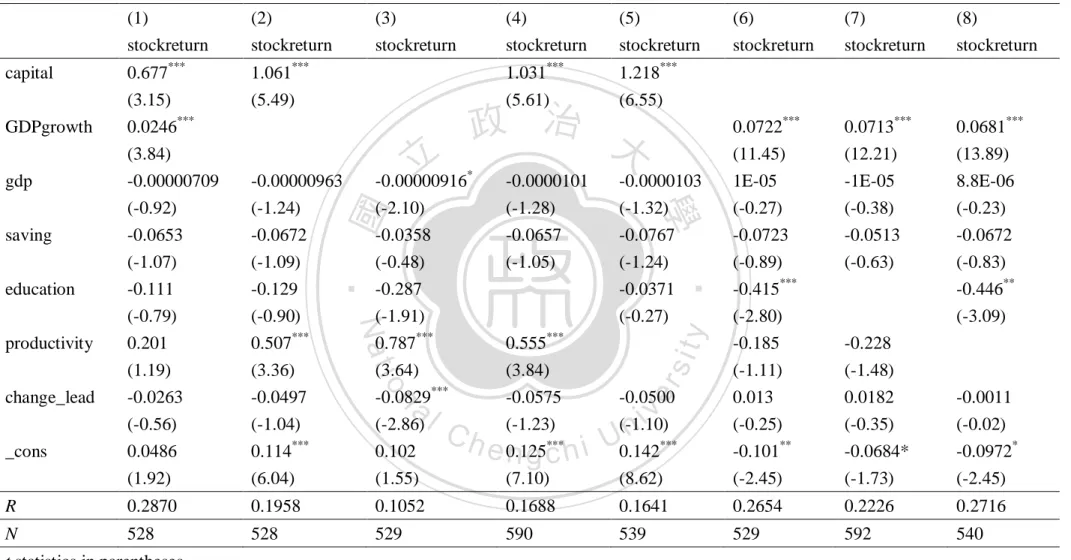
(33) point increase in output. As a result, we think that the education exactly has highly correlation with productivity, so we prefer not to put these two variables into the model at the same time. We take them as substitutes to avoid the collinearity problem. Since the World Competitiveness Center editing the national competitiveness rank takes the real GDP growth as a hard data criterion, and hard criteria represent a weight of 2/3 in the overall ranking, we know that the economy performance correlates with the national competitiveness rank significantly. As what we expected, there exists significant correlation between the real GDP growth and the change of national. 政治大 at the same time to avoid the insignificant problem of beta caused by collinearity. 立. competitiveness. As a result, we prefer not to take these two variables into the model. Overall, there still exist some correlation between the variables, but because the. ‧ 國. 學. correlation value is not as high as we mention previously, and we do not think they. ‧. will cause the problem to this study if we do not take them into account.. y. Nat. io. sit. 4.3 Empirical result. n. al. er. In order to decide which model has better explanation, we do the Hausman test. i n U. v. first. And we find that in model (1) , the Hausman test suggests us using the random. Ch. engchi. effect model. On the other hand, in the other models, through Hausman test, the evidence of fixed effect exists so we decide to use the fixed effect model for model (2) to model (8). Table 4 illustrates the research results for all the models we set. In all the models, we set country stock return as the dependent variables. In the model (1) we put all the variables into the model, and according to table 4, we could find that the real GDP growth is significant, which represents that real GDP growth exactly has positive influence on the stock market return, and it also fits our expectation at first. And the capital formation is significantly positive to the stock return in all of the models. In 28.

(34) this model we find other variables are not significant. We think this may result from the real GDP growth which is highly correlated with other variables. Last but not least, we do not find that the change of national competitiveness has significant effect on the stock market return in spite of the sign of the coefficient that fits our expectation. As a result, there may exist some collinearity problems if we put them into the model at the same time. In the next models, we try to take the real GDP growth away, and try to solve the collinearity problem. In the model (2), we take the real GDP growth variable away, and we find that this. 政治大 supports (CRR, 1986), that the industrial production is a source of common variation 立 time the productivity has positive effect on the stock return significantly, which. to the stock market return. And this is the most different part from the model (1).. ‧ 國. 學. After we take away the real GDP growth variable, the capital formation is still. ‧. positive and significant to the stock market return.. sit. y. Nat. In the model (3), we try to take both the capital formation and real GDP growth. io. er. variables away at the same time. We find that the change of national competitiveness has a positive effect on the stock market return. When the national competitiveness. al. n. v i n rank improves, the stock marketC will have a better performance next year significantly. hengchi U This also fits our original expectation. On the other hand, the productivity still has positive effect on the stock market return significantly. In the model (4), we take the real GDP growth and education variables away, and find that the capital formation and productivity are positive to the stock market return significantly. Other variables are not significant. In the model (5), we take the real GDP growth and productivity variables away, and the only significant variable is the capital formation. Finally, we also try to use the time effect and cross-sectional effect model for all the models we build, we use the dummies for each countries to test the time effect and 29.

(35) cross-sectional effect in the OLS model, but there are not obvious time effect or cross-sectional effect in our models.. 立. 政治大. ‧. ‧ 國. 學. n. er. io. sit. y. Nat. al. Ch. engchi. 30. i n U. v.

(36) Table 4 Regression results for stock return and related variables (1) stockreturn. (2) stockreturn. 0.677*** (3.15) 0.0246*** (3.84). 1.061*** (5.49). -0.00000709 (-0.92) -0.0653. -0.00000963 (-1.24) -0.0672. -0.00000916* (-2.10) -0.0358. -0.0000101 (-1.28) -0.0657. (-1.07) -0.111 (-0.79) 0.201. (-1.09) -0.129 (-0.90) 0.507***. (-0.48) -0.287 (-1.91) 0.787***. (-1.05). (1.19) -0.0263 (-0.56). (3.36) -0.0497 (-1.04). (3.64) -0.0829*** (-2.86). (3.84) -0.0575 (-1.23). -0.0500 (-1.10). 0.0486 (1.92). 0.114*** (6.04). 0.102 (1.55). ***. ***. R. 0.2870. 0.1958. N. 528. 528. al. 1.031*** (5.61). 1.218*** (6.55). Ch. 0.0713*** (12.21). 0.0681*** (13.89). -0.0000103 (-1.32) -0.0767. 1E-05 (-0.27) -0.0723. -1E-05 (-0.38) -0.0513. 8.8E-06 (-0.23) -0.0672. (-1.24) -0.0371 (-0.27). (-0.89) -0.415*** (-2.80) -0.185. (-0.63). (-0.83) -0.446** (-3.09). (-1.11) 0.013 (-0.25). (-1.48) 0.0182 (-0.35). -0.0011 (-0.02). -0.0684* (-1.73). -0.0972* (-2.45). y iv. n U i en 0.125 0.142 gch. -0.228. (7.10). (8.62). -0.101** (-2.45). 0.1052. 0.1688. 0.1641. 0.2654. 0.2226. 0.2716. 529. 590. 539. 529. 592. 540. t statistics in parentheses *. 0.0722*** (11.45). 0.555***. n. _cons. 立. io. change_lead. (8) stockreturn. 政治大. Nat. productivity. (7) stockreturn. ‧. education. (6) stockreturn. 學. saving. (5) stockreturn. sit. gdp. (4) stockreturn. er. GDPgrowth. ‧ 國. capital. (3) stockreturn. p < 0.1, ** p < 0.05, *** p < 0.01 31.

(37) In the model (6), (7), and (8), we find that the real GDP growth variables are all positive to the stock market return significantly. And the real GDP variable is extremely significant. We could proof that the economic growth is a factor, which really has significant influence on the stock market return. In the model (6) and (8) we also find the education variable is significant in model (6) and model (8), but the sign of coefficient is negative, and it implies that the education has a negative effect on the stock market return. But in all the other models, the education variables is not significant and also has a negative effect on the stock market returns. We also try to use the lag period of education variables, but the result is not significant. Only when we use the education as a contemporaneous variable is the result significant, but the direction does not fit our expectation. It may be caused by. 治政大 is a long-term process. make the result unexpected. On the other hand, the education 立 It could not immediately response on the country. The education expenditure of a. the incomplete data we collect, that is, there exist some missing values of our data and. ‧ 國. 學. country may response on the stock market or on national competitiveness after several periods, that is, the education expenditure is a lag variable in the models. As a result,. ‧. it seems not significant in our models.. We could find that the education expenditure will not reflect on the stock market. y. Nat. sit. return in short period, but we trust that the education expenditure is a long-term. al. er. io. variable to reflect on the stock market return. Owing to the data period is only. n. fourteen years, we do not have the enough evidence to prove the education. Ch. i n U. v. expenditure will affect the stock market return. In the future, if there are other. engchi. researcheres interested in this topic may collect much longer data to do further researches.. 32.

(38) Chapter5 Conclusion In this research, we find that the real GDP growth has a positive effect on the stock market return significantly; this offer a supporting to solve the puzzle that economic growth is good to the stock market return. It also fit the research of Faugère, C. and J. V. Erlach (2006), Ibbotson and Chen (2003). We trust the real GDP growth is a good variable to the stock market return and it is also a good index to predict the stock market return, and investors could use it to choose a good investment target in the future. But we still should take notice that the real GDP growth is a long term process. It is not a short period index. We should take it as a long term index to choose the stock markets, and this also fits our goal to earn the long term market return instead of only short term return caused by the event shocks. 政治大 Although only in the model 立 (3) is the national competitiveness change significant. or other unpredictable factors.. ‧ 國. 學. to the stock market return, in other models the national competitiveness change still has the right direction to the stock market return, that is when a nation has improvement on its national competitiveness, it will bring a positive effect for the. ‧. next few years. We could expect that raising the national competitiveness is good to. y. Nat. the stock market. National competitiveness has a positive effect on the stock market. io. sit. return, and this offers a good reason for government to maintain the national. er. competitiveness. This research tell us that the stock market could not reflect the. al. n. v i n C reflect on the stockUmarket return for stockholders. national competitiveness could noth engchi. short-term condition but the short-term condition, and this is also the reason why the. Our research also provides a good index for investors to choose a good target. stock market to invest. When the international investors or institution try to search good investment target, they could take the real GDP growth rate and the national competitiveness index into account to pick good stock market to invest. We also find that the intercept of our models are significant, this may imply there still exist some factors which we do not take into our model. This research supports the classical Solow Growth Model, and is also consistent with Faugère, C. and J. V. Erlach (2006), Ibbotson and Chen (2003). We use nearly all stock market data of the world, and we prove that the real GDP growth will have a good impact on the stock market return. The real GDP growth is a good index to fit all the stock markets of the world, not only focusing on some developed or emerging 33.

(39) markets. Our research result is different from Ritter(2005), Ritter find that there are negative relationship between the stock return and per capita GDP growth, and this may cause from the data period, Ritter’s research data is from 16 countries and the time period is from 1900-2002. Compare to our data, Ritter’s data is longer and the data goes through many different economic time period, on the other hand, our data goes through the period which global economic grow rapidly. This may induce we have the different conclusions for the economic growth and stock return issue. This research also finds that the capital formation has positive effect on the stock market return, and the productivity is also an important factor, which will influence the stock market return. On the other hand, the education is not a factor which will influence the stock market return. It may be caused by the data collecting. 治政大does not reflect on the stock its influence in short period. The education expenditure 立 market return contemporaneously. It takes time to have an effect on the stock market. incompleteness or the fact that the education is a long term factor, and we may not see. ‧ 國. 學. All in all, we know that the economic growth is an important factor to the stock market return. The international investor and institution could have better investment. ‧. return if they could find a country which has a good economic growth in the long term, such that, for more than 5 years or even 10 years.. y. Nat. sit. Our data is mainly from World Competitiveness Center of IMD and DataStream.. al. er. io. These databases are almost having the detailed data and nearly nothing omitted. Some. n. data is not completed, hard to collect, or the data period is too short to use. As a result,. Ch. i n U. v. we delete data of some countries which are not long enough or have too many missing. engchi. values. We try best to collect all the data we can find and make all the data keep its true value. We should keep in mind that in the future, the world markets are opening continually, and this may induce the interact effect of each country, especially when the national competitiveness rank is a relative concept. We do not take the interact effect of each country into our study, and this may be a future research direction for researchers. The national competitiveness statistical data is still not long enough, and there are nearly two hundred countries all around the world, the IMD statistical data may not be enough because it only includes complete data about fifty countries. The future research may try to use the other famous statistic institution, the World Economic Forum, which also does the rank about the national competitiveness. We do not take 34.

(40) the systematic risk factor into account in this research. The future research may try to put the systematic risk factor of each country into the model.. 立. 政治大. ‧. ‧ 國. 學. n. er. io. sit. y. Nat. al. Ch. engchi. 35. i n U. v.

(41) Reference 1.. Anderson, C. W., L. G.-F. O, 2006, "Empirical Evidence on Capital Investment, Growth Options, and Security Returns" Journal of Finance 62, 171-192.. 2.. Banz, Rolf W., 1981, "The relationship between return and market value of common stocks" Journal of Financial Economics 9, 3-18.. 3.. Barro, R., Sala-i-Martin, X., 1992, "Convergence" Journal of Political Economy 100, 223-251.. 4.. Barro, R., Sala-i-Martin, X., 1995, "Economic Growth" McGraw Hill, New York.. 5.. Begg, 1999, " Cities and Competitiveness" Urban Studies 36. 5/6 : 795-809. 6.. Berk J. B., R. C. Green, V. Naik, 1999, " Optimal Investment, Growth Options, and. 7.. 政治大 Bhandari, 1988, "Debt/Equity Ratio and Expected Common 立 Empirical Evidence", Journal of Finance 43, No. 2, 507-528. 8.. Bodurtha, J., James N., D. C. Cho, 1989, "Economic forces and the stock market:. Security Returns", Journal of Finance54, Issue 5, 1553-1607. Stock Returns:. ‧ 國. 學. An international perspective" Global Finance Journal 1, 21-46. Burton A. Weisbrod, 1962, "Education and Investment in Human Capital" Journal. ‧. 9.. of Political Economy 70, No. 5, 106-123. y. Nat. sit. 10. Chen, N., R. Roll and S. Ross, 1986, "Economic Forces and the Stock Market.". al. er. io. Journal of Business 59, 383-403.. n. 11. Clark J. , Guy K., 1998, " Innovation and competitiveness: a review", Technology. Ch. i n U. v. Analysis & Strategic Management, Vol 10, issue 3, 363-395. engchi. 12. Eugene F. Fama and Kenneth R. French, 1992, "The Cross-Section of Expected Stock Returns", The Journal of Finance, Vol. 47, No. 2, 427-465 13. Fama E. and French K., 1993, "Common risk factors in the returns on stocks and bonds" Journal of Financial Economics, 3-56. 14. Faugère, C., J. V. Erlach, 2006, "The Equity Premium: Consistent with GDP Growth and Portfolio Insurance" The Financial Review 41, 547-564. 15. Garcia V. F. and Liu L., 1999, "macroeconomic determinant of stock market development" Journal of Applied Economics, Vol. II, No. 1, 29-59 16. Georghiou L. G., J. S. Metcalfe, "Evaluation of the impact of European community research programmes upon industrial competitiveness", R&D Management Volume 23, Issue 2, 161-170. 36.

(42) 17. Levine, R., Renelt, D., 1992, "A sensitivity analysis of cross-country growth regressions" The American Economic Review 82, 942-963. 18. Lu Zhang, 2005, " The Value Premium", Journal of Finance, Volume 60, Issue 1, 67-103 19. Mankiw, G., Romer, D., Weil, D., 1992, "A contribution to the empirics of economic growth." Quarterly Journal of Economics 107, 407-437. 20. Moretti, E., 2004, "Workers' Education, Spillovers, and Productivity: Evidence from Plant-Level ProductionFunctions." The American Economic Review 94 (3), 656-690. 21. Myoung-jae Lee, 2002, "Panel Data Econometrics, Methods of Moments and Limited Dependent Variables.". 治政 and the empirics of economic growth for OECD大 countries." Quarterly Journal of 立 Economics 111, 943-953.. 22. Nonneman, W., Vanhoudt, P., 1996, "A further augmentation of the Solow model. ‧ 國. 學. 23. Porter M.E., 1990, " The competitive advantage of nations: with a new introduction" 24. Rapkin, DP and J, R. Strand, 1995, "Competitiveness: useful concept, political. ‧. slogan or dangerous obsession", International Journal of Political Economy Yearbook, 8, 1-20.. y. Nat. sit. 25. Ritter, J. R., 2005, "Economic Growth and Equity Returns" Pacific-Basin Finance. al. er. io. Journal 13, 489-503.. n. 26. Roger G. Ibbotson and Peng Chen, "Long-Run Stock Returns: Participating in the. Ch. i n U. v. Real Economy", Financial Analysts Journal ,Vol. 59, No. 1: 88-98. engchi. 27. 陳冠位, 2002, "Study on the Evaluation System of City Competitiveness." ,博士論文 28. 薛瀾, 1995, “從國際競爭力評估美國在全球競爭地位”，美歐月刊，pp.44-60。. 37.

(43) Appendix Sample Country List Argentina. Denmark. Ireland. Netherlands. South Africa. Australia. Finland. Israel. New Zealand. Spain. Austria. France. Belgium. Germany. Brazil. Greece. Canada. Hong Kong. Chile. Hungary. China Mainland. Iceland. Colombia. India. Czech Republic. Indonesia. Sweden Switzerland. Philippines. Taiwan. Korea. Poland. Thailand. Lithuania. Portugal. Turkey. Luxembourg. Russia. United Kingdom. Malaysia. Slovak Republic. USA. Mexico. Slovenia. y. sit. n. er. io. al. ‧. Nat. Jordan. 學. ‧ 國. 治 Italy 政大Norway Peru 立Japan. Ch. engchi U. 38. v i n. Venezuela.

(44)