國
立
交
通
大
學
光電工程學系
碩
士
論
文
超大反常色散摻鉺鎖模光纖雷射的脈衝特性研究
Pulse characteristics of long-cavity-length
mode-locked Er-doped fiber laser in the anomalous
dispersion regime
研 究 生:楊良愉
指導教授:賴暎杰 教授
誌謝
來到交大這兩年,是我人生當中最充實的時光之一,碩一修習不少有關 光電相關的課程,在這些課程裡有學到許多寶貴的知識,也讓我這位從數 學領域跨行過來的門外漢得以一窺這項門兼具工程和物理的高深學門。在 此也要感謝諸位授課老師的醍醐灌頂。 特別感謝賴老師在這兩年對我的啟發,不論是做事的方法,還有培養思 考的方式無處不令人感到佩服。也謝謝老師平時教導光學和雷射上的觀 念,,還有 Meeting 上老師介紹的一些量子效應還有量子傳輸等,這些新奇 有趣的研究工作,讓我大開眼界。 實驗室方面有堅強的博班團隊當作火車頭,負責引領著我們這些小碩班 在此感謝曉山學長在實驗上給予專業的指導,並且適時的給予鼓勵還有幫 忙,讓我們不致於那麼孤軍奮戰,碩一剛進來也經常受學長照顧。謝謝尚穎 學長充當我的理論顧問,每當有理論上的困惑,坐在隔壁的他就會馬上放 下手邊工作,然後隨手拿起一本書並說著:你說的現象,應該是在這個部 分。謝謝聖閔總是能指出我做事方法的矛盾點,而使我不走冤妄路,是個說 話相當豪爽且中肯的人。超級謝謝阿甘學長傳承被動鎖模雷射的精隨。國 豪總是帶來歡樂,還有教會我人與人相處的智慧,以及股票市場的爾虞我 詐,當然少不了在 LOL 遊戲上經常跑到上路幫我 gank 敵人。謝謝國豪的勉 勵,在關鍵時刻總是給人安定感。賴賴也經常帶上家裡做的小點心給我這個貪吃鬼享用,還有分享專業的光柵知識,當然還有超級有頭腦的遊戲交 易技巧。耀德阿斌也常常幫我分擔一些雜物,讓我輕鬆不少感謝感謝。已 畢業的學長姐們小柏、家弘、子祥、那美克夫婦、秀鳳、佩芳、小愛、宏 傑也常常回實驗室跟我們玩耍聊天打牌讓人感到非常溫馨。 也要謝謝我 的父母,在背後默默支持。最後要感謝我的女朋友,謝謝妳陪我走過碩班生 涯,有妳的鼓勵和貼心,碩士班生涯中多了感動和驚喜。
摘要
本論文研究一個由 400m 長單模光纖組成共振腔的被動摻鉺鎖模光纖雷射, 我們藉由偏振疊加波鎖模的機制來鎖模產生鎖模雷射脈衝,並使用 30/70 的 光耦合器把 70%的能量輸出腔外,剩下的 30%傳回腔內做來維持共振,輸出的 脈衝重複頻率為 500kHz。此雷射藉由調整共振腔內的偏振控制器可達到不 同的穩定鎖模狀態,像是長方波和短脈衝輸出等。在方波操作條件下,單一 個雷射脈衝能量最高可以達到 142J,並且方波寬度隨著幫浦能量增加而呈 現線性遞增的趨勢,在此過程中方波不會因幫浦能量加大而遭破壞,此正是 方波操作狀態下的一大特色,其優點是可以獲得大脈衝能量而持續穩定。 此雷射的雙波長現象也是個有趣的狀態,其輸出包含方波和短脈衝兩種 狀態的疊合,不論是在時域或是頻域上皆可觀測到兩脈衝疊加的跡象,我們 藉由腔外濾波器去選取此狀態的特定頻段,可以定性上去驗證確實是兩個 狀態疊加。 另外我們感到興趣的是分別在短脈衝和方波操作狀態下,輸出脈衝的頻 譜相位分布特性。我們藉由實驗上光濾波後的脈衝寬度量測結果來估算頻 域二階啁啾與三階啁啾的大小,也同時對濾波後的短脈衝來進行壓縮實驗, 藉由色散補償光纖設法將其壓縮至 160 皮秒以下,然後使用光自相干涉儀來 量測脈衝寬度。
Abstract
This thesis work mainly studies Er-doped passive mode-locked fiber laser configuration. The cavity length mainly consists of 400 meters-long single mode fiber and 1.65 meters long Er-doped gain fiber. We use the polarization additive pulse mode-locking (P-APM) technique to mode-lock the laser. An optical output coupler with the ratio of 30/70 (30% power back into the cavity) is used to extract the optical pulses and the pulse repetition rate is 500 kHz. By adjusting the polarization controller inside the cavity, we can produce different stable mode-locked states including the long square pulse state and the short pulse state. In the square pulse operation regime, a single pulse can reach the pulse energy of 142 nJ by increasing the pump power. The pulse-width increases proportionally without the pulse breaking.
Dual-wavelength phenomenon is another interesting mode-locked state of the laser. It is a combination of two different pulse states: one is the short pulse state and the other is the square pulse state. We filter the optical spectrum to observe the changes of the pulse shape in the time domain to confirm their properties.
We are also interested in the analysis of the spectral chirp characteristics in both the square pulse and short pulse regimes by sliding-filtering the pulses. We filter the spectra of the optical pulses in the two different mode-locked regimes and record the resulting pulses in the time domain. The spectral 2nd and 3rd order chirps are estimated based on the measurement results. In the meantime, we try to compress the filtered optical pulses by connecting a section of dispersion compensation fiber (DCF) and different lengths of single mode fiber (SMF). The optical pulse-width was measured by an autocorrelator and the minimum
Contents
誌謝 ... i
摘要 ... iii
Abstract ... iv
Contents ... vi
List of Figures and Tables ... viii
Chapter 1 Introduction ... 1
1.1 The history of mode-locked laser ... 1
1.2 Motivation ... 3
1.3 Organization ... 4
Reference ... 6
Chapter 2 Principle of passive mode-locked fiber laser ... 8
2.1 Master equation in the active mode-locking regime ... 8
2.2 Fast saturable absorber mode-Locking ... 11
2.3Addittive pulse mode-locking (APM) ... 14
2.4 Square pulse generation ... 16
2.5 High order chirp ... 18
Chapter 3 Experimental results of long-cavity length mode-locked fiber lasers 23 3.1 Pulse characteristics measurement ... 23
3.1-1 Experimental setup ... 23
3.2-1 In the square pulse regime ... 29
3.2-2 In the short pulse regime... 34
3.3 Dual-wavelength phenomenon... 43
3.4 Pulse compression results ... 46
Chapter 4 Conclusion and future work ... 56
Future work ... 58
List of Figures
Fig. 2. 1 The gain distribution of different modes with linear loss [2.1] ... 9
Fig. 2. 2 Schematic of passively mode-locked laser with a fast saturable absorber and the time dependence of the pulse and the net gain ... 11
Fig. 2. 3 The scheme of APM ... 14
Fig. 2. 4 Rotation of elliptical polarization in an isotropic Kerr-medium ... 15
Fig. 2. 5 Transmission in the cases of and [2.9] ... 17
Fig. 3. 1 Experimental setup of the long-cavity length fiber laser and the output pulse measurement………23
Fig. 3. 2 (a) Square pulse measured by oscilloscope (b) Optical spectrum in the square pulse regime ... 25
Fig. 3. 3 (a) Output power versus pump power (b) Square pulses in different pump power (c) Pulse-width of square pulses and output power in different pump power ... 25
Fig. 3. 4 (a) Short pulse measured by oscilloscope (b) Optical spectrum of the short pulse ... 28
Fig. 3. 5 Experimental setup of the spectral filtering method ... 29
Fig. 3. 6 The square pulse measured by oscilloscope ... 29
Fig. 3. 7 Optical spectrum with filter bandwidth~1.6nm in square pulse regime ... 31
Fig. 3. 8 Different optical bands with central wavelength from 1558.7nm to 1569.9nm ... 31 Fig. 3. 9 Pulses corresponding to different filter bands and central wavelengths
Fig. 3. 10 Pulse-widths corresponding to different bands in Fig. 3.8 and its
fitting parabolic curve with coefficients ... 32 Fig. 3. 11 Results from different FBWs (1nm, 1.6nm, 2nm) in the same square
pulse regime ... 34 Fig. 3. 12 Pulse measured by oscilloscope ... 35 Fig. 3. 13 Optical spectrum of pulse and filter bands with their FCW. ... 36 Fig. 3. 14 Optical spectrum with filter bandwidth~3nm in the short pulse regime
... 36 Fig. 3. 15 Pulses corresponding to bands in Fig. 3.14 ... 37 Fig. 3. 16 Pulse-width corresponding to different bands in Fig. 3.14 and the
fitting curve (dash line) ... 38 Fig. 3. 17 Pulse measured by oscilloscope. ... 40 Fig. 3. 18 Optical spectra of pulses and filter bands with their FCW. ... 40 Fig. 3. 19 Optical spectra with filter bandwidth~0.4nm in short pulse regime .. 41 Fig. 3. 20 Pulse-width corresponding to different bands in Fig. 3.19 and fitting
parabolic dash curve (dash line) ... 41 Fig. 3. 21 Pulses corresponding to the bands in Fig. 3.19 ... 42 Fig. 3. 22 Step-like pulse measured by oscilloscope ... 44 Fig. 3. 23 Five optical bands with different central wavelengths in the same filter bandwidth (8.65nm) ... 44 Fig. 3. 24 Pulses corresponding to bands in Fig. 3.23 ... 46 Fig. 3. 25 (a) Short pulse measured by oscilloscope (b) Optical spectrum in short
pulse regime (c) Compressed pulse-width with the use of DCF 174 m ……….48 Fig. 3. 26 Experimental setup for pulse compression with band-pass filtering .. 49 Fig. 3. 27 (a) Optical spectrum of filtered pulses after passing through
Er-amplifier (b) Filtered pulse measured by oscilloscope
corresponding to band (red solid line) shown in Fig. 3.27 (a)………50 Fig. 3. 28 Autocorrelation measurement of pulse in the use of DCF 174 m +SMF
0.5 km (a)Left hand side of the pulse (b)Right hand side of the pulse ... 51 Fig. 3. 29 Autocorrelation measurement with the use of DCF 174 m +SMF 1 km
(a)Left hand side of the pulse (b)Right hand side of the pulse ... 52 Fig. 3. 30 Autocorrelation measurement with the use of DCF 174 m (a)Left hand side of the pulse (b)Right hand side of the pulse ... 52 Fig. 3. 31 Pulses measured by oscilloscope after passing through DCF 174 m
and SMF 0, 0.5, 1 km ... 53 Fig. 3. 32 Trace of width from autocorrelation and oscilloscope ... 53
List of Tables
Table 3. 1 Numerical values of pulse-width corresponding to different bands in Fig. 3.9 and the fitting coefficients for the parabolic dash curve in Fig. 3.10 ... 33 Table 3. 2 Numerical values of pulse-width corresponding to different bands in
Fig. 3.14 and the fitting coefficients for the linear dashed line in Fig. 3.16 ... 38 Table 3. 3 Numerical values of pulse-widths corresponding to different bands in
Fig. 3.20 and fitting coefficients of parabolic dash curve ... 42 Table 3. 4 Numerical values of the pulse-width in Fig. 3.25 ... 49 Table 3. 5 Numerical values of Fig. 3.32 ... 54
Chapter 1
Introduction
1.1 The history of mode-locked laser
Mode-locked lasers can generate short optical pulses and have been found useful in many applications such as optical communication, optical signal processing, two-photon microscopy, and laser surgery. The term “mode-locking” means making the relative phases of the longitudinal modes existing inside the laser to be fixed so that the laser can generate short output pulses (nanosecond to femtosecond and further smaller). Mode-locked lasers can be roughly classified into two categories: passive and active. Passive mode-locked lasers usually use slow or fast saturable absorbers to achieve the mode-locking while active mode-locked lasers use a modulator to achieve the mode-locking. There are many types of mode-locked lasers, such as solid-state bulk lasers (usually based on ion-doped crystals or glasses), fiber lasers, and semiconductor lasers (mostly for applications in optical fiber communication).The development of mode-locking techniques started from 1960s. First indication of mode-locking appeared in the work of Gürs and Müller [1.1], [1.2] on ruby lasers, and Statz and Tang [1.3] on He–Ne lasers. Hargrove [1.4] first achieved mode-locking by adding internal loss modulation inside the resonator. This was the case of active mode-locking.
Mocker and Collins [1.5] showed that the saturable dye used in ruby lasers to
Q-switch the laser could also be used to achieve mode-locking. He observed that
train of short pulses separated by the roundtrip time and each pulse shares the same energy. This is the first example of passive mode-locking.
The theory of active mode-locking was established by Siegman and Kuizenga [1.6]. The scheme was to put a loss modulator to achieve the injection locking of the axial modes in the frequency domain. He predicted that the pulse shape was Gaussian in this scheme. On the other side, the theory of passive mode-locking was stimulated by the CW mode-locking of dye lasers [1.7]. But the relaxation time of the absorber was much longer than the pulse generated in the laser. This has stimulated H. A. Haus to establish the theory of passive mode-locking with a slow saturable absorber [1.8].
In 1989, E. P. Ippen, H. A. Haus, and L. Y. Liu established a simple model of additive pulse mode-locking (APM) [1.9]. The APM mechanism utilizes the self-phase modulation in an auxiliary cavity to produce pulse shortening in the main laser by coherent interference at the coupler mirror. The APM technique was later used in fiber ring lasers where the APM effect was produced by the nonlinear birefringent effect in the resonator. By tuning the polarization controllers, the pulse is split into two polarization components which interfere at the polarizer to effectively produce fast saturable-absorber action.
In 1980s Mears et al developed the first Erbium-Doped fiber Laser [1.10] [1.11]. Since then the fiber laser researches have drawn serious attention in the world. Unlike most other types of lasers, the laser cavity made of fiber is constructed monolithically by fusion splicing different types of fibers.
There are several types of fiber lasers, using different gain fibers such as erbium, ytterbium, neodymium, dysprosium, and thulium. Several types of methods have also been developed for passive mode-locking the fiber lasers:
mode-locking (P-APM) configurations and nonlinear optical loop mirrors (NOLM).
1.2 Motivation
Fiber lasers had been widely used for different applications. In particular, high pulse energy lasers have been used in coherent lidar systems, range finding, remote sensing and industrial processing applications. A low-repetition-rate optical pulse train with a sub megahertz repetition rate is useful for many applications such as micromachining, biomedical diagnostics, and lidar systems. Examples of such low-repetition-rate pulse lasers are Q-switched lasers [1.12] and SESAM lasers [1.13].
In many applications such as fluorescence lifetime imaging measurements and high-resolution lidar systems, a short pulse (picosecond to sub nanosecond) is required. Passively mode-locked lasers can generate ultrashort pulse-width (picosecond to sub nanosecond) but the pulse repetition rate is still too high for those systems. Conventional methods to reduce the repetition rate of mode-locked lasers are to use a modulator driven by an external electric signal as a pulse picker. But this kind of system is complicated and expensive and the power efficiency is also low. The best way to lower the repetition rate is to extend the cavity length [1.14].
In solid-state lasers [1.15], using the multiple-pass technique to construct a long laser cavity was not so easy in comparison to fiber lasers. The fiber lasers have advantages on their alignment free, compact size, and low maintenance cost.
mode-locked fiber lasers. In an early experiment, the repetition rate was reduced to 1.7 MHz with the pulse energy in the order of nano joule in a mode-locked fiber laser configuration [1.16]. Later, there were some reports on highly-chirped pulses in the anomalous or all normal dispersion ring cavity fiber lasers that delivered higher energy operating at approximately hundreds of kHz [1.17], [1.18], [1.19]. But these lasers are difficult in alignment and also time-consuming in comparison to the using of fibers as the laser cavity.
To conquer these disadvantages, extending the fiber laser cavity length is a good choice.
1.3 Organization
This thesis contains four chapters. Chapter1 gives the history of mode-locked laser in the development of experiments and theories, from solid state lasers to fiber lasers. Then we introduce the motivation of researching the long-cavity mode-locked fiber laser.
In chapter 2, we give a quick derivation for the master equation in the active mode-locking regime. Then we replace the active modulation term by the self-amplitude modulation term to describe the fast absorber scheme in passive mode-locking. In chapter 2.3, we introduce additive the original pulse mode-locking technique (APM), which requires the use of two resonators and the output pulse was from the interference of the output pulses of each resonator. Then we explain the principle of Polarization APM (P-APM) mode-locking, which is a method without requiring an additional cavity, but by utilizing the nonlinear phase shifts of the two circular polarization states inside the fiber cavity.
In chapter 2.4, we introduce how the square pulse can be generated in the passive mode-locked fiber laser.
In chapter 2.5, we first show the characteristics of chirped Gaussian pulses in the linear chirp case only. Then we extend the formula to the second and third order chirp cases.
In chapter 3, we use the nonlinear polarization rotation to achieve an all-fiber mode-locked laser with a 400m-long single mode fiber as the main cavity. We show the experiment results of generating square pulses and also its stability by increasing the pump power, and short pulse. In chapter 3.2, we use the spectral filtering method to study the pulse characteristics in the square pulse and short pulse regimes. In chapter 3.3, the dual-wavelength phenomenon is observed. We characterize it to be the additive of the square pulse and the short pulse. In chapter 3.4, experiment results of pulse compression on the filtered pulses will be demonstrated.
Finally, the conclusion of the thesis work and possible future work in the future is given in chapter 4.
Reference
[1.1] K. Gürs and R. Müller, “Breitband-modulation durch Steuerung der emission eines optischen masers (Auskopple-modulation),” Phys. Lett., vol. 5, pp. 179–181, 1963. [1.2] K. Gürs, “Beats and modulation in optical ruby lasers,” in Quantum Electronics III, P.
Grivet and N. Bloembergen, Eds. New York: Columbia Univ. Press, pp. 1113–1119, 1964.
[1.3] H. Statz and C. L. Tang, “Zeeman effect and nonlinear interactions between oscillating laser modes,” in Quantum Electronics III, P. Grivet and N. Bloembergen, Eds. New York: Columbia Univ. Press, pp. 469–498, 1964.
[1.4] L. E. Hargrove, R. L. Fork, and M. A. Pollack, “Locking of He–Ne laser modes induced by synchronous intractivity modulation,” Appl. Phys. Lett., vol. 5, pp. 4–6, 1964
[1.5] H. W. Mocker and R. J. Collins, “Mode competition and self-locking effects in a Q-switched ruby laser,” Appl. Phys. Lett., vol. 7, pp. 270–272, 1965.
[1.6] D. I. Kuizenga and A. E. Siegman, “Modulator frequency detuning effects in the FM mode-locked laser,” IEEE J. Quantum Electron., vol. QE-6, pp. 803–808, 1970.
[1.7] E. P. Ippen, C. V. Shank, and A. Dienes, “Passive mode locking of the cw dye laser,” Appl. Phys. Lett., vol. 21, pp. 348–350, 1972.
[1.8] H. A. Haus, “Theory of mode locking with a fast saturable absorber,” J. Appl. Phys., vol. 46, pp. 3049–3058, 1975.
[1.9] E. P. Ippen, H. A. Haus, and L. Y. Liu, “Additive pulse mode locking,” J. Opt. Soc. Amer. B, Opt. Phys., vol. 6, pp. 1736–1745, 1989.
[1.10] R. J. Mears, L. Reekie, I. M. Jauncey, D. N. Payne “Low-noise erbium-doped fibre amplifier operating at 1.54μm,” Electron. Lett., vol. 23, pp. 1026-1028 , 1987.
[1.11] I. M. Jauncey, L. Reekie, R. J. Mears, D. N. Payne, C. J. Rowe, D. C. J. Reid, I. Bennion, C. Edge. “Narrow-linewidth fibre laser with integral fibre grating,” Electron.
Lett., vol. 22, pp. 987, 1986.
[1.12] U. Sharma, C. S. Kim, and J. U. Kang, “Highly stable tunable dual-wavelength Q-switched fiber laser for DIAL applications,” IEEE Photon. Technol. Lett., vol. 16, pp.1277 , 2004.
[1.13] L. Chen, M. Zhang, C. Zhou, Y. Cai, L. Ren and Z. Zhang, “Ultra-low repetition rate linear-cavity erbium-doped fibre laser modelocked with semiconductor saturable absorber mirror,” Electron. Lett., vol. 23, pp. 1026-1028 , 2009.
[1.14] A. Killi, J. Dörring, U. Morgner, M. J. Lederer, J. Frei,and D. Kopf, “High speed electro-optical cavity dumping of mode-locked laser oscillators,” Opt. Express 13, pp. 1916-1922, 2005.
[1.15] S. H. Cho, B. E. Bouma, E. P. Ippen, and J. G.Fujimoto, “Low-repetition-rate high-peak-power Kerr-lens mode-locked TiAl2O3 laser with a multiple-pass cavity,” Opt. Lett., vol. 24, pp. 417-419 , 1999.
[1.16] K. H. Fong, S. Y. Kim, K. Kazuro, H. Yaguchi, and S. Y. Set, “Generation of low-repetition rate high energy picosecond pulses from a single-wall carbon nanotube mode-locked fiber laser,” Opt. Amp. and Appl. Conf., paper OMD4, 2006.
[1.17] W. H. Renninger, A. Chong, and F. W. Wise, “Highly-chirped dissipative solitons in anomalous-dispersion fiber lasers,” CLEO., paper CTuFF6, May 2008,
[1.18] W. H. Renninger, A. Chong, and Frank W. Wise, “Giant-chirp oscillators for short-pulse fiber amplifiers,” Opt. Lett., vol. 33, pp. 3025–3027, 2008
[1.19] S. Kobtsev, S. Kukarin, and Y. Fedotov, “Ultra-low repetition rate mode-locked fiber laser with high-energy pulses,” Opt. Express, vol. 16, pp. 21936–21941, 2008.
Chapter 2
Principle of passive mode-locked fiber
laser
2.1 Master equation in the active
mode-locked regime
We follow the treatment in the paper by H. A. Haus, (“Mode-Locking of Lasers”, [2.1]) to derive the mater equation for explaining the mode-locking mechanism. The following equation shows the optical field amplitude change of the n-th mode in each roundtrip pass. The first term in the right hand side means the change of the n-th mode after passing through the gain medium and the linear loss of the whole cavity. The second term is caused by the amplitude modulator in each roundtrip. is the amplitude of the n-th mode,
The following two terms show how the modulator makes the (n-1)-th and (n+1)-th modes contribute to the n-th mode after modulation.
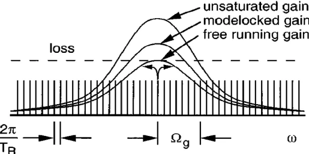
Fig. 2.1 shows the gain profile and linear loss. The modes which experience positive net gain ( -loss) can exist in the cavity.
Fig. 2.1 The gain distribution of different modes with linear loss [2.1]
The following three assumptions will be used:
(1) The frequency dependent gain can be expanded to second order of . (2) Discrete frequency spectrum is replaced by a continuum spectrum, as a
continuous function of .
supposing that the spectrum is dense.
We can get a differential equation describing mode-locking for the amplitude change per round trip.
In steady state, , we can get a Gaussian pulse solution, which demonstrates how a mode-locked pulse can be formed theoretically.
2.2 Fast Saturable Absorber
Mode-Locking
Fig. 2.2 Schematic of passively mode-locked laser with a fast saturable absorber and the time dependence of the pulse and the net gain
In passive mode-locked lasers, the modulator was replaced by a saturable absorber. The theoretical model was first developed by H. A. Haus in the reference [2.2], who had done fantastic work in the fast saturable absorber
mode-locking theory. When the relaxation time of the absorber was much longer than the pulse generated in the laser, the slow saturable absorber mode-locking theory needs to be used [2.3].
Here we first introduce the simple model to explain how the fast saturable absorber works. First, the transmission function is given by the follow
expression:
(2.2-1) where
If the saturation is relatively weak, we can expand this formula by Taylor expansion.
, is the effective area of the mode. Thus the
transmission function becomes
, e is the self-amplitude modulation (SAM) coefficient. We replace the active modulator term by the fast saturable absorber term in the master equation (2.2-1), and the term merge into the loss l term. We finally have
.
This second order differential equation simply described the mechanism of fast saturable absorber mode-locking. The solution is a hyperbolic secant function of time:
, where
and . is the pulse-width and we can see that it is inverse proportional to the gain bandwidth and proportional to peak gain .
2.3 Addittive Pulse Mode-Locking
(APM)
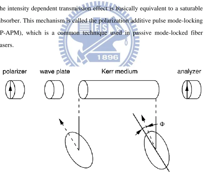
The additive pulse mode-locking is a technique for passive mode-locked lasers [2.4] and is usually used to generate pulses with the width from picosecond to femtosecond [2.5], [2.6]. The early APM techniques contained two resonators as shown in Fig. 2.3. It was later found that the APM effect can be also achieved in a single resonator cavity by utilizing the two light polarizations. This is illustrated in Fig. 2.4.
Fig. 2.3 The scheme of APM
From Fig. 2.4, the linearly polarized light is transformed into the elliptically polarized light by a wave plate. It then passes through an isotropic Kerr–medium which will rotate the elliptically polarized light by an intensity dependent angle. If the output light is again linearly polarized by an analyzer, the output light of the system will be intensity dependent. In this way this effect realizes an equivalent fast saturable absorber. It is a good method for the fiber laser systems since all the components in this scheme can be made as the fiber-optic type.
Consider the two circularly polarized eigen-modes in the nonlinear fiber [2.7] as follows:
(2.3-1) Here are the fields of two circularly polarized waves and is the Kerr nonlinearity coefficient. Equation (2.3-1) shows how these two polarization states affect each other in the Kerr medium. It also shows that both circular polarization modes acquire different phase shifts that are proportional to intensities. The angle of the elliptic polarization will rotate an angle as shown in Fig. 2.4 [2.7]. When the elliptic polarization light passes through the analyzer, the intensity dependent transmission effect is basically equivalent to a saturable absorber. This mechanism is called the polarization additive pulse mode-locking (P-APM), which is a common technique used in passive mode-locked fiber lasers.
2.4 Square pulse generation
Nanosecond square pulses can be generated in the Er-doped mode-locked fiber laser with a long cavity. This is due to the peak power clamping effect [2.8].
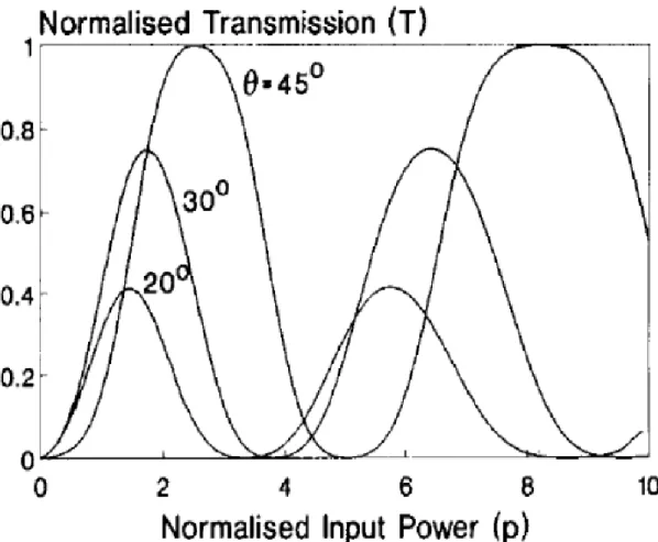
Equation (2.4-1) shows that the round trip transmission of the light depends on , the beat length of the birefringent element, the cavity length L and the azimuth angle of the polarization-dependent isolator with respect to the fast axis. Here is the rotation angle of the polarization controllers. The net transmission is a nonlinear function of the power as shown in Fig 2.5. It is caused by the nonlinear polarization rotation (NPR) effect.
( 2 . 4 - 1 ) The effective beat length will change with the input power, as indicated by equation (2.4-2). is the power dependent beat length
(2.4-2) This will be contained in the equation (2.4-3) and thus affect the power dependent switching power .
(2.4-3) Equation (2.4-3) shows how L and are related to the switching power
. We can find that a longer cavity length results a lower switching power. This is also the reason why square pulses are much easier generated in a long
fiber cavity.
Fig. 2.5 shows the simulation normalized transmission T in the cases of
and . When the transmission profiles
do not have a flat top shape. But when , the power peaks near p=2.5 and p=8.5 clearly exhibit a flat top. So it means by adjusting the polarization controllers one can change the transmission profile, letting the system operated in the flat top power range to generate square pulses.
2.5 High Order Chirp
Considering a Gaussian pulse with a linear chirp , the electric field in the spectral domain with normalize amplitude can be written as
If is the inverse Fourier transform of , i.e., the time domain electric field, then
The variable is determined by the spectral width. We can use the following equation (2.5-1) to calculate by substituting into the full-width-half-maximum spectral width, :
(2.5-1) Since
the Gaussian shape pulse has the pulse-width given by
It shows how the linear spectral chirp term contributes to the time domain width. This is the main effect why the optical pulses get wider in fibers. If , the optical pulse is called transform limited. The time bandwidth product for a Gaussian pulse becomes
Now we want to estimate the second order chirp of the pulse. The idea comes from the linear chirp case. We consider a Gaussian pulse with a linear chirp and a second order chirp (caused by third order dispersion). The electric field in the spectral domain with normalize amplitude is given by equation (2.5-2), assuming in the moving frame of the pulse.
(2.5-2) Supposing that is small enough, let us multiply the electric field by a
narrowband filter function with a central frequency . Denoting
and expanding the phase term to third order around the filter central frequency by Taylor expansion, one has:
We will neglect the third order term in the right hand side by assuming is small enough. We will also assume the filter bandwidth is much narrower than the pulse spectral width.
Thus
phase shift, and the term leads to a shift in time domain. Thus we can simplify the expression for IFT as follows:
where . The pulse-width in the time domain will be
(2.5-3) where (in the unit of second square) and
(in the unit of inverse of second square). Here is given by and is the filter band width in the unit of nm. is the difference of the central wavelength of the pulse and the central wavelength of the filtered optical band in angular frequency. We should note that the central frequency of original
spectral field is zero (2.5-2), therefore and .
Suppose is much smaller than . By neglecting the term in equation (2.5-3), one has
(2.5-4) We get a simple formula to describe the higher order chirp effect on the filtered pulses. The relation in equation (2.5-4) predicts that the filtered pulse-width will have a linear dependence with the filter central wavelength if there is a second order chirp.
Now we extend the formula to more general case which including third order spectral chirp. Similarly, we first consider the following electric field equation
(2.5-5) Let the electric field multiply a filter function with a central wavelength which is , then we expand the phase term to second order term by Taylor expansion around the filter central frequency and do the Inverse Fourier Transform translating the spectral field to electric field in time domain. The resulted pulse-width in time domain is given by,
(2.5-6) Equation (2.5-6) give the pulse-width of filter band which have a filter band central frequency difference to central frequency to original spectrum, i.e. . By expanding (2.5-6) in the power series of and neglecting third order term and higher order terms of it, we can get the following equation that is parabolic function to .
Reference
[2.1] H. A. Haus, “Mode-Locking of Lasers,” IEEE J. Selected Topics Quantum Electron. vol. 6, pp. 1173-1185, 2000.
[2.2] H. A. Haus, “Theory of mode locking with a fast saturable absorber,” J. Appl. Phys., vol. 46, pp. 3049–3058, 1975.
[2.3] E. G. Arthurs, D. J. Bradley and A. G. Roddie, “Buildup of picosecond pulse generation in passively mode-locked rhodamine dye lasers,” Appl. Phys. Lett., vol. 23, pp. 88–90, 1973.
[2.4] E. P. Ippen, H. A. Haus, and L. Y. Liu, “Additive pulse mode locking,” J. Opt. Soc. Am., vol. 6 , pp. 1736 , 1989.
[2.5] J. Mark, L. Y. Liu, K. L. Hall, H. A. Haus, and E. P. Ippen, “Femtosecond pulse generation in a laser with a nonlinear external resonator”, Opt. Lett., vol. 14 , Issue 1, pp. 48-50 , 1989.
[2.6] J. Chen, J. W. Sickler, E. P. Ippen and F. X. Kärtner, ” High repetition rate, low jitter, low intensity noise, fundamentally mode-locked 167 fs soliton Er-fiber laser,” Opt. Lett., vol. 32, pp. 1566-1568, 2007.
[2.7] H. A. Haus and E. P. Ippen, “Mode-locked Fiber Ring Lasers,” OSA TOPS on Ultrafast Electronics and Optoelectronics, vol.13, pp. 6-12, 1997
[2.8] Y. Li, X. Gu, M. Yan, E. Wu and H. Zeng, “Square nanosecond mode-locked Er-fiber laser synchronized to a picosecond Yb-fiber laser,” Opt. Express, vol. 17, pp. 4526-4532, 2009.
[2.9] V. J. Matsas, T. P. Newson, D. J. Richardson, D. N. Payne, “Self-starting passively mode-locked fiber ring soliton laser exploiting nonlinear polarization rotation,” Electron. Lett., vol. 28, pp. 1391-1393, 1992.
Chapter 3
Experimental results of long-cavity
length mode-locked fiber lasers
3.1 Pulse measurement
3.1-1 Experimental setup
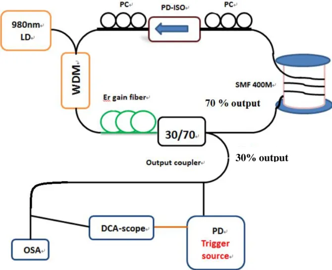
Fig. 3.1 Experimental setup of the long-cavity length fiber laser and the output pulse measurement
Our experiment setup is illustrated in Fig. 3.1. The fiber laser system is
pumped by 980nm diode lasers. The pump lights are coupled into the fiber cavity by using WDM couplers. We use a 1.65 meter long, Er-doped gain fiber with the pump absorption coefficient of 80 dB/m. The 400 m single mode fiber (SMF)contributes to the main cavity length. The cavity also contains two polarization controllers and one polarization dependent isolator to implement the nonlinear polarization rotation technique for achieving mode-locking.
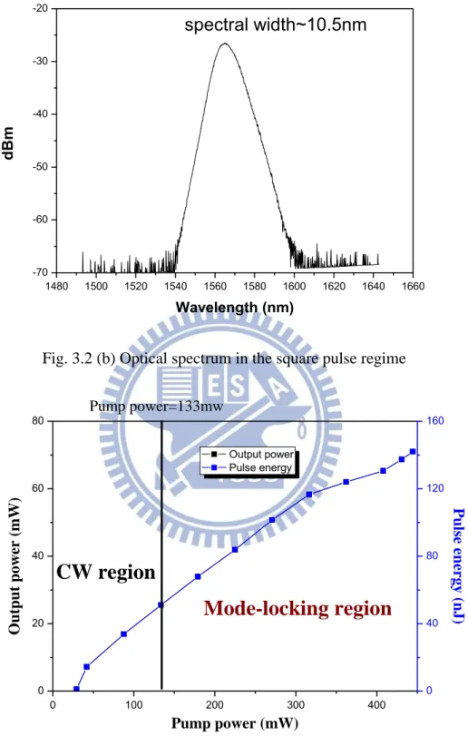
The generated square pulse is shown in Fig. 3.2 (a), which has the pulse-width of 3.57 ns. The optical spectrum is shown in Fig. 3.2 (b) with the spectral width of 10.5 nm. 0 5 10 15 20 0.0000 0.0005 0.0010 0.0015 0.0020 0.0025 In ten si ty (W att) Time (nanosecond) pulsewidth~3.576ns
1480 1500 1520 1540 1560 1580 1600 1620 1640 1660 -70 -60 -50 -40 -30 -20 dBm Wavelength (nm) spectral width~10.5nm
Fig. 3.2 (b) Optical spectrum in the square pulse regime
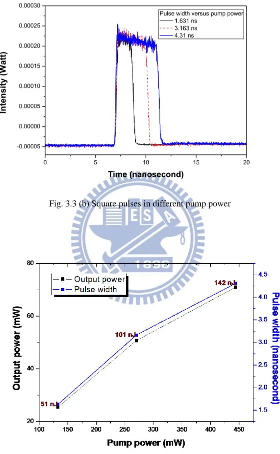
0 100 200 300 400 0 20 40 60 80 Output power Pulse energy Pump power (mW) Ou tp u t p owe r ( m W) 0 40 80 120 160 Pul se e n er gy ( n J) Pump power=133mw
Mode-locking region
CW region
0 5 10 15 20 -0.00005 0.00000 0.00005 0.00010 0.00015 0.00020 0.00025 0.00030 In ten si ty (W att) Time (nanosecond)
Pulse width versus pump power 1.631 ns
3.163 ns 4.31 ns
Fig. 3.3 (b) Square pulses in different pump power
Fig. 3.3(a) shows that the output power is increasing linearly with the pump power. Fig. 3.3 (b) and Fig. 3.3 (c) shows that the width of output square pulse is increasing linearly with the pump power while peak power of the square pulses remain constant. The mode-locked region starts at 133 mW pump power and remains mode-locked at least till the pump power of 450 mW (limited by our available pump power). The obtained maximum pulse energy of 142 nJ breaks the record in [3.1.1], which only has the highest pulse energy of 120 nJ without pulse breaking.
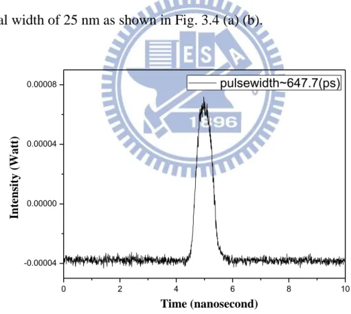
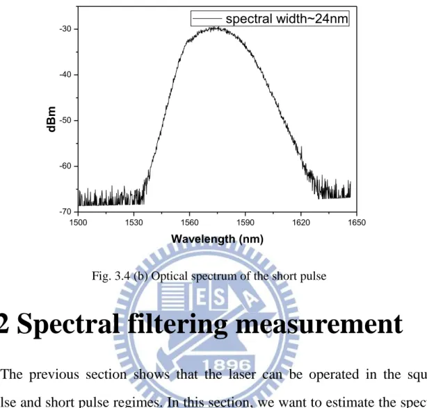
At the pump power of 133 mw and the output power of 21 mw, this laser can also produce short pulses with the pulse-width of 647 ps and with a much wider spectral width of 25 nm as shown in Fig. 3.4 (a) (b).
0 2 4 6 8 10 -0.00004 0.00000 0.00004 0.00008 In te n sity ( Wat t) Time (nanosecond) pulsewidth~647.7(ps)
1500 1530 1560 1590 1620 1650 -70 -60 -50 -40 -30 dBm Wavelength (nm) spectral width~24nm
Fig. 3.4 (b) Optical spectrum of the short pulse
3.2 Spectral filtering measurement
The previous section shows that the laser can be operated in the square pulse and short pulse regimes. In this section, we want to estimate the spectral linear chirp and second order chirp characteristics of the laser output pulses by sliding-filtering the optical spectrum.
3.2-1 In the square pulse regime
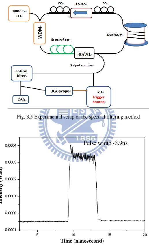
Fig. 3.5 Experimental setup of the spectral filtering method
5 10 15 20 -0.0001 0.0000 0.0001 0.0002 0.0003 0.0004 In te n sity ( Wat t) Time (nanosecond) Pulse width~3.9ns
Fig. 3.5 shows the experimental setup for measuring the filtered pulses. Fig. 3.6 showed the original square pulse with the pulse-width of 3.9 nanosecond. We put an external optical filter outside the cavity to filter the pulse shown in Fig. 3.6. By selecting the different optical bands as shown in Fig. 3.7 and 3.8, the resulted pulses are recorded by the oscilloscope as shown in Fig. 3.9
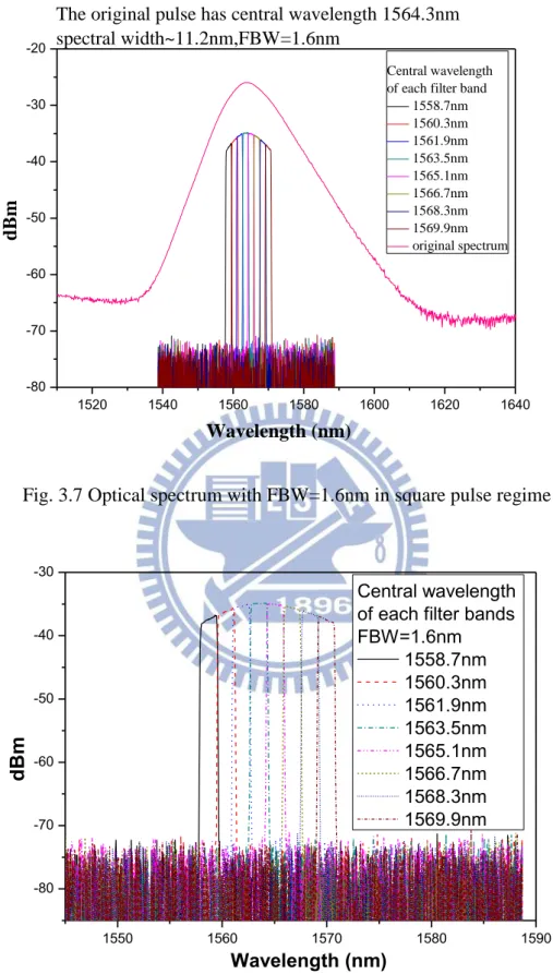
The original spectrum has the spectral width of 11.2 nm in Fig. 3.7. The central wavelength is at 1564.3nm. By using a filter bandwidth (FBW) of 1.6nm and by varying the filter central wavelength (FCW) from 1558.7 nm to 1569.9 nm, the resulted pulses are shown in Fig. 3.9. We can observe that these nanosecond filtered pulses still maintain square pulse-like shapes.
In Table 3.1, the numerical values of the pulse-width have a concave down parabolic-like trace versus the central wavelength of the band-pass filter as illustrated in Fig. 3.10. It is caused by linear chirp and second order chirp and third order chirp. We should note that the FCWs have been shifted in another reference frame as shown in Fig. 3.10. The 1564.3 nm is shifted to 0 nm, so does other filter bands. The blue dash line is the fitting parabolic curve of the black solid line and the fitting coefficients are put in Table 3.1 and we will use them to calculate these spectral chirp parameters by result of Chap 2.5. These calculated chirp parameters is shown in Table 3.2. Linear chirp is in the unit of square of seconds (s).We can observe that the largest pulse-width occurs in the bands near the central wavelength.
1520 1540 1560 1580 1600 1620 1640 -80 -70 -60 -50 -40 -30 -20
The original pulse has central wavelength 1564.3nm spectral width~11.2nm,FBW=1.6nm
d
Bm
Wavelength (nm)
Central wavelength of each filter band
1558.7nm 1560.3nm 1561.9nm 1563.5nm 1565.1nm 1566.7nm 1568.3nm 1569.9nm original spectrum
Fig. 3.7 Optical spectrum with FBW=1.6nm in square pulse regime
1550 1560 1570 1580 1590 -80 -70 -60 -50 -40 -30 dBm Wavelength (nm) Central wavelength of each filter bands FBW=1.6nm 1558.7nm 1560.3nm 1561.9nm 1563.5nm 1565.1nm 1566.7nm 1568.3nm 1569.9nm
0 10 20 0.0000 0.0003 0.0006 0.0000 0.0003 0.0006 0.0000 0.0003 0.0006 0.0000 0.0003 0.0006 0.0000 0.0003 0.0006 0.0000 0.0003 0.0006 0.0000 0.0003 0.0000 0.0003 0 10 20 In te n si ty ( Watt ) Time (nanosecond) 1558.7nm 1560.3nm 1561.9nm 1563.5nm 1565.1nm 1566.7nm 1568.3nm 1569.9nm
Fig. 3.9 Pulses corresponding to different filter bands and central wavelengths in Fig. 3.8
-6 -4 -2 0 2 4 6 3.55 3.60 3.65 3.70 3.75 3.80 3.85 3.90 Pu lsewi d th (n s)
Shifted central wavelenth (nm) Pulsewidth
Polynomial Fit of pulsewidth
Model Polynomial Adj. R-Sq 0.9629 Value Standard pulsewidt Interce 3.880 0.0109 pulsewidt B1 -0.01 0.00195 pulsewidt B2 -0.00 6.10784E FBW=1.6nm Central wavelength=1564.3nm
Table 3.1 Numerical values of pulse-width corresponding to different bands in Fig. 3.9 and the fitting coefficients for the parabolic dash curve in Fig. 3.10
Central wavelength(nm) Pulse-width(nanosecond)
-5.6 3.781 -4 3.842 -2.4 3.877 -0.8 3.885 0.8 3.856 2.4 3.806 4 3.747 5.6 3.562
Fitting coefficients Fitting curve
Intercept(ns) 3.88088
(ns/nm) -0.01674
(ns/nm^2) -0.00643
Table 3. 2 Calculated spectral chirp parameters of Fig. 3.10
In square pulse regime FBW=1.6nm
Linear chirp (S^2)
Second chirp (S^3)
1561 1562 1563 1564 1565 1566 1567 1568 1569 3.80 3.85 3.90 3.95 4.00 4.05 Pu lse wi d th (n s) (n s) Wavelength (nm) fiter bandwidth1.6nm fiter bandwidth1nm fiter bandwidth2nm
Fig. 3.11 Results from different FBWs (1nm, 1.6nm, 2nm) in the same square pulse regime
Fig. 3.11 shows the filtered pulse-widths in the square pulse regime. We filter the spectrum in three different FBWs (1nm, 1.6nm, 2nm) in order to observe their difference in the trace of pulse-width. In Fig. 3.11 we can find that these traces of pulse-width in three different FBWs are almost similar to each other. They are all like concave down parabolic shape curves and the maximum values occur near the central wavelength 1564 nm, which are the same as in Fig. 3.10.
3.2-2 In the short pulse regime
regime. There are two different cases. One is in the condition of FBW=3 nm and the other is with FBW=0.4 nm.
Fig. 3.12 shows the original short pulse with the pulse-width of 660 ps. Fig. 3.13 is the filtered spectrum containing seven filter bands and the original spectrum of the pulse is also shown in Fig. 3.13, which is with the 1569 nm central wavelength and the 24 nm spectral width. In Fig. 3.14, the filter bands are across the range of 24 nm with each FBW=3nm. The tops of these bands are 30 dB above the noise floor.
0 2 4 6 8 10 0.0000 0.0001 0.0002 0.0003
pulse width~660ps
In ten si ty (W att) Time (nanosecond)1500 1520 1540 1560 1580 1600 1620 1640 -70 -60 -50 -40 -30
The original pulse has central wavelength 1569nm spectrum width~24nm,FBW=3nm
d
Bm
Wavelength (nm)
Central wavelength of each filter bands
1560nm 1563nm 1566nm 1569nm 1572nm 1575nm 1578nm original spectrum
Fig. 3.13 Optical spectrum of pulse and filter bands with their FCW. 1540 1560 1580 1600 -70 -60 -50 -40 -30 dBm Wavelength (nm) FBW=3nm and FCW= 1560nm 1563nm 1566nm 1569nm 1572nm 1575nm 1578nm
0 5 10 -0.0001 0.0000 0.0001 0.0002 -0.0001 0.0000 0.0001 0.0002 -0.0001 0.0000 0.0001 0.0002 -0.0001 0.0000 0.0001 0.0002 -0.0001 0.0000 0.0001 0.0002 0.0000 0.0001 0.0002 0.0000 0.0001 0.00020 5 10 In ten si ty (W att) Time (nanosecond) 1560nm 1563nm 1566nm 1569nm 1572nm 1575nm 1578nm
Fig. 3.15 Pulses corresponding to bands in Fig. 3.14
Fig. 3.15 shows the measurement results of different bands in the time domain. In Fig. 3.16 we find the pulse-width increase linearly as we tune the filter band to longer wavelengths. This linear line trace is due to the effect of linear chirp and second order chirp. The short vertical error bar across points is the standard deviation of these data. The dashed linear line is the fitting result. Table 3.3 lists the numerical values in Fig. 3.16 and fitting coefficients of linear red dash line. Table 3.4 lists the linear chirp (in the unit of square of second) and second order chirp parameters (in the unit of cubic of second) calculated from fitting
coefficients in Table 3.3 -8 -4 0 4 8 300 350 400 450 500 Pu lsewi d th (p s) Wavelength (nm) Pulsewidth
Linear Fit of Pulsewidth
Equation y = a + Adj. R-Sq 0.9805
Value Standard Pulsewidt Interce 401.84 2.67404 Pulsewidt Slope 8.6171 0.49431
Fig. 3.16 Pulse-width corresponding to different bands in Fig. 3.14 and the fitting curve (dash line)
Table 3.3 Numerical values of pulse-width corresponding to different bands in Fig. 3.14 and the fitting coefficients for the linear red dash line in Fig. 3.16
Central wavelength(nm)
Of each filter band Pulse-width(picosecond) STD(picosecond)
1560 316.24 11.97474 1563 352.7 7.16066 1566 384.125 16.7597 1569 406.5167 10.92223 1572 421.0313 9.01592 1575 458.7313 16.55687 1578 480.8875 32.15489 Fitting coefficient Fitting curve Intercept(ps) 401.84868
Table 3. 4 Calculated spectral chirp parameters in Fig. 3.16
In short pulse regime FBW=3nm
Pulse-width (ps) 650
Central wavelength 1569 nm
Spectral width 24 nm
Linear chirp (S^2)
Second chirp (S^3)
The following experiment is another case of mode-locked short pulse state and we use FBW=0.4 nm. Fig. 3.17, 3.18, and 3.19 show a 734 picosecond pulse with the central wavelength of 1572 nm and the spectral width of 24 nm. Each filtered spectrum have a Gaussian like shape with a narrow FBW=0.4nm. Noting that we shift the central wavelength = 1572 nm to 0 nm as in Fig 3.20 by horizontal shift. The total thirteen FBWs give rise to the pulse-widths in Fig. 3.20 and the pulse shapes in Fig. 3.21, which show the saturation of the pulse-width after 3 nm. In the region of 1560 nm to 1576 nm, the pulse-width still maintains linear increasing. Here the most different thing is the use of a much smaller FBW than the previous case. We use the parabolic dash line to fit the trace of pulse-width in Fig. 3.20. The fitting coefficients of parabolic trace and the values of pulse-width are shown in Table 3.5 and we use these coefficients to calculate the linear chirp (in the unit of square of second) and second order chirp (in the unit of cubic of second) which are shown in Table 3.6.
0 2 4 6 8 10 0.0000 0.0002 0.0004 0.0006 In te n sity ( Wat t) Time (nanosecond) Pulse width=734ps
Fig. 3.17 Pulse measured by oscilloscope
1500 1520 1540 1560 1580 1600 1620 1640 -70 -60 -50 -40 -30 -20
The original pulse has central wavelength 1572nm spectral width~24nm,FBW=0.4 nm d Bm Wavelength (nm) Original spectrum 1558nm 1560nm 1562nm 1564nm 1566nm 1568nm 1570nm 1572nm 1574nm 1576nm 1578nm 1580nm 1582nm 1584nm 1586nm
1560 1570 1580 -70 -60 -50 -40 -30 -20 dBm Wavelength (nm) FBW=0.4nm FCW 1560nm 1562nm 1564nm 1566nm 1568nm 1570nm 1572nm 1574nm 1576nm 1578nm 1580nm 1582nm 1584nm
Fig. 3.19 Optical spectrum with FBW=0.4 nm in short pulse regime
-15 -10 -5 0 5 10 15 300 400 500 600 700 Pu lse wi d th 1 (p s) Wavelength (nm) Pulse width1
Polynomial Fit of pulse width1
Model Polynomi
Adj. R-Squ 0.99737
Value Standard Er
pulse width Intercept 554.700 12.72628
pulse width B1 12.6645 1.19322
pulse width B2 -0.5375 0.16657
Fig. 3.20 Pulse-width corresponding to different filtered bands in Fig. 3.19 and the fitting parabolic dash curve (dash line)
0 5 10 0 5 10 In ten si ty (W att) Time (picosecond) 1562nm 1564nm 1566nm 1568nm 1570nm 1572nm 1574nm 1576nm 1578nm 1580nm 1582nm 1584nm 1586nm
Fig. 3.21 Pulses corresponding to bands of Fig. 3.19
Table 3.5 Numerical values of pulse-widths corresponding to different bands in Fig. 3.20 and fitting coefficients of parabolic dash curve
Wavelength(nm) Pulse-width(picosecond) STD 1560 319 26.13 1562 358 26.7 1564 413 32.45 1566 460 36.6 1568 493 39.5 1570 528 49.2 1572 565 47 1574 586.4 45.9 1576 593.5 43.6 1578 612.3 7.8 1580 606.93 64.6 1582 608.84 81.8 1584 601 81.5
Fitting coefficient Fitting curve
Intercept(ps) 554.70015
(ps/nm) 12.66458
(ps/nm^2) -0.53751
Table 3.6 Calculated spectral chirp parameters of Fig. 3.20
In short pulse regime FBW= 0.4 nm
Pulse-width (ps) 647.7 Central wavelength 1572 nm Spectral width 24 nm Linear chirp (S^2) Second chirp (S^3)
3.3 Dual-wavelength phenomenon
The dual-wavelength phenomenon in a long-cavity mode-locked Er-fiber laser was first reported in [3.2].They used a 730 m long cavity length mode-locked Er-doped fiber laser with the utilization of the NPR technique. The authors observed two spectral humps in a stable mode-locked state. Then they used a band-pass filter to filter each hump and found that each hump corresponds to different rectangular pulses. They proved that the spectrum was consisting of two rectangular pulses.
5 10 15 20 0.0000 0.0002 0.0004 0.0006 0.0008 0.0010 In ten si ty (W att) Time (nanosecond)
Fig. 3.22 Step-like pulse measured by oscilloscope
1500 1530 1560 1590 1620 1650 -90 -80 -70 -60 -50 -40 -30 dBm Wavelength (nm) FCW 1587.9nm 1579.4nm 1570.5nm 1565.83nm 1557.15nm original spectrum
Fig. 3.23 Five optical bands with different central wavelength in the same filter bandwidth (8.65nm)
In this section, we use the same method to investigate this problem by using the band-pass filter to filter out each hump at once. In Fig. 3.22, the step like nanosecond pulse is measured by the oscilloscope. Its spectrum is shown in Fig. 3.23 with five FBWs and FCWs. We can observe two humps (1564 nm and 1594 nm) in the spectrum. By filtering its spectrum, we record the time domain pulses in Fig. 3.24, corresponding to different bands in Fig. 3.23.
From Fig. 3.23, we choose theband center at 1565.83 nm with FBW=8.65 nm and the obtained square pulse become the largest. When we choose the band center at 1557.15nm and 1587.9nm with same FBW=8.65 nm. The square pulse is now not obvious. In the other side, the short pulse is almost in every band. Fig. 3.22 also gives a clear picture about the peak of the short pulse and the rectangular shape pulse. Since the spectrum of the short pulse is much wide (spectral width=0~40nm) than the spectrum of the square pulse (spectrum width =10~15 nm) in this laser, when we scan the spectrum, the short pulse is not easy to disappear totally but the other is. From these data, we can conclude that this interesting state is the combination of the short pulse and square pulse states.
-10 0 10 0.0000 0.0004 0.0000 0.0004 0.0008 0.0000 0.0004 0.0008 0.0000 0.0004 0.0008 0.0000 0.0002 0.0004 -10 0 10 In tesi ty (W att) Time (ns) 1587.9nm 1579.4nm 1570.5nm 1565.83nm 1557.15nm
Fig. 3.24 Pulses corresponding to bands in Fig. 3.23
3.4 Pulse compression
In this section, we try to compress the short pulse to achieve the possible minimum pulse-width. First we let the laser operate in the short pulse regime, which has the spectral width of 25 nm in Fig. 3.25 (b) and the pulse-width of 509 picosecond in Fig. 3.25 (a). Then we connect a section of dispersion compensation fiber with the length of 174 meters long (DCF 174 m), which can
measured pulse-width is 510 picosecond and almost unchanged. So we try to connect the DCF 174 m with different lengths of SMF fibers to reduce the normal dispersion values. Fig. 3.25 (c) shows the measured pulse-widths.
From Fig. 3.25 (c), the minimum pulse-width happens at the case of DCF 174 m+ SMF 800 m. The minimum pulse-width is about 348 picosecond from Table 3.7 and the compressing ratio is 0.71(min width/max width). The curve in Fig. 3.25 (c) shows linearly decreasing in width in the beginning and then it gets saturated. This experiment result indicates that the higher order chirp effects are very significant since the pulse-width can not be compressed down to the transform limited value. Actually it is very far from the transform limited pulse-width. 0 2 4 6 8 10 0.0000 0.0002 0.0004 0.0006 0.0008 0.0010 In te n sity ( Wat t) Time (nanosecond) Pulse width 509ps Fig. 3.25 (a) Short pulse measured by oscilloscope
1500 1520 1540 1560 1580 1600 1620 1640 -70 -60 -50 -40 -30 d Bm Wavelength (nm) Spectral width~26nm Central wavelength~1568.9nm
Fig. 3.25 (b) Optical spectrum in short pulse regime
0 200 400 600 800 1000 340 360 380 400 420 440 460 480 500
520 The minimum pulsewidth occur in the use of DCF 174m+SMF 500m~800m
Compressing ratio:0.71(min/max width)
Pul se wid th ( p s) DCF174m+SMF 100*x (m)
Table 3. 7 Numerical values of the pulse-width in Fig. 3.25 (c) DCF174m+SMF x m Pulse-width(picosecond) 0 510 100 476.8 200 441.6 300 413.7 400 391.5 500 369.42 600 361.7 700 355.2 800 348 900 380.4 1000 393
From the above results, we try to use the optical filter to reduce high order chirp effects by choosing a FBW as narrow as possible. Fig. 3.26 shows the schematic setup. The band-pass filter is used to filter the laser output pulse. The filtered pulse is a short pulse with the width of 230 ps, shorter than the original pulse as expected. Then the filtered pulse passes through the DCF 174 m+SMF fibers with the SMF=0, 0.5, 1 kilometer long. Since most of the pulse energy is lost after filtering, we put an Er-doped fiber amplifier to amplify the filtered pulse in order to measure it by an autocorrelator.
1480 1500 1520 1540 1560 1580 1600 1620 -70 -60 -50 -40 -30
Filter band bear 1555.5nm FBW=0.1nm d Bm Wavelength (nm) After AMP After filter
Fig. 3.27 (a) Optical spectrum of filtered pulses after passing through Er-amplifier
0 2 4 6 8 10 -0.0001 0.0000 0.0001 0.0002 0.0003 0.0004 0.0005 Pulsewidth=230ps In ten si ty (W att) Time (nanosecond)
In Fig. 3.27 (a), black dash line is the optical spectrum of filtered pulse after it passing through the Er-doped fiber amplifier and red solid line the optical spectrum of filtered pulse before it passing through the Er-doped fiber amplifier. The peak is the original filter band located at 1555.5nm with FBW=0.1nm. The bottom of the curve comes from the ASE noises of the optical amplifier. Fig. 3.28, 3.29, and 3.30 are the autocorrelation measurements in the use of DCF 174 m and SMF 0, 0.5, 1 kilometer long. Fig. 3.28 (a) records the left hand side of the pulse and Fig. 3.28 (b) records the right hand side of the pulse. The peak is a spike which may be caused by the higher order chirp of the pulse or may be the coherent spike of the pulse. We can take it as the central of the autocorrelation trace. Since the time window of our autocorrelator is about 220 picosecond wide, the pulse-width is still too wide for the measurement window. Therefore we measure the pulse in two sides. One is on the left hand side of spike and the other is on right hand side by tuning the delay of the autocorrelator. The upper line in Fig. 3.28 is the top of the trace and the lower line is the half height of trace. In this way we can use the two half height widths of the traces to estimate the pulse-width. 0 100 200 300 400 500 600 700 0.00 0.01 0.02 0.03 0.04 0.05 In ten si ty Time (picosecond)
Left hand side of pulse Half hight Top 0 100 200 300 400 500 600 700 0.00 0.02 0.04 0.06 0.08 In ten si ty Time (picosecond)
Right hand side of pulse Half hight
Top
Fig. 3.28 Autocorrelation measurement of pulse in the use of DCF 174 m +SMF 0.5 km (a)Left hand side of the pulse (b)Right hand side of the pulse
0 100 200 300 400 500 600 700 0.00 0.01 0.02 0.03 0.04 0.05 0.06 0.07 In te nsi ty Time (picosecond) Left hand side of pulse Half hight Top 0 100 200 300 400 500 600 700 0.00 0.02 0.04 0.06 0.08 0.10 In te nsi ty Time (picosecond)
Right hand side of pulse Half hight
Top
Fig. 3.29 Autocorrelation measurement of pulse in the use of DCF 174 m +SMF 1 km (a)Left hand side of the pulse (b)Right hand side of the pulse
0 100 200 300 400 500 600 700 0.004 0.006 0.008 0.010 0.012 0.014 In te n si ty Time (picosecond)
Left hand side of pulse Half hight Top 0 100 200 300 400 500 600 700 0.002 0.004 0.006 0.008 0.010 0.012 0.014 0.016 0.018 0.020 0.022 In te nsi ty Time (picosecond)
Right hand side of pulse Half hight
Top
Fig. 3.30 Autocorrelation measurement of pulse in the use of DCF 174 m (a)Left hand side of the pulse (b)Right hand side of the pulse
0 5 10 -0.0001 0.0000 0.0001 0.0002 0.0003 0.0004 0.0000 0.0002 0.0004 0.0006 0.0000 0.0002 0.0004 0 5 10 Time (nanosecond) DCF+SMF0.5km In ten si ty (W att) DCF Pulse width230ps Pulse width186ps Pulse width200ps DCF+SMF1km
Fig. 3.31 Pulses measured by oscilloscope after passing through DCF 174 m and SMF 0, 0.5, 1 km 0.0 0.2 0.4 0.6 0.8 1.0 1.2 140 150 160 170 180 190 200 210 220 230 after AMP SMF0.5km SMF1km Pu lsewi d th (p s) DCF174m+SMF x (km) Osilloscope Autocorrelation
Table 3.8 Numerical values of Fig. 3.32
Pulse-width(ps) Autocorrelation
DCF 174 m 230 204
DCF 174 m+ SMF 0.5 km 186 143
DCF 174 m+ SMF 1 km 200 190
Fig. 3.32 gives the trace of pulse-width in cases of different SMF lengths. The trace shows that the minimum pulse-width occurs near the case of SMF=0.5 km and the minimum pulse-width is about 130~140 picosecond. Although in Fig. 3.29 (a) and Fig. 3.30 (a), the left hand sides of the pulse are not recorded completely, limited by autocorrelation window, we can still take the edges of half height to get the estimated value. Table 3.8 listed the numerical values of Fig. 3.32. The results demonstrate for the first time that the highly chirped pulse from the long cavity length mode-locked Er-fiber fiber can still be compressed down to the 100ps level by a simple scheme. Further compression may also be possible if more precise pulse shaping techniques can be used.
References
[3.1] Y. C. Lai and L. H. Kan, “High energy pulse generation in large negative-dispersion mode-locked Er-doped fiber laser with long cavity length,” National Digital Library of Theses and Dissertations inTaiwan, 2011.
[3.2] D. Mao, X. Liu, L. Wang, H. Lu and L. Duan, “Dual-wavelength step-like pulses in an ultra-large negative-dispersion fiber laser,” Opt. Express, vol.19, Issue.5, pp.3996-4001, 2011.
Chapter 4
Conclusion and future work
Square nanosecond pulses and short picosecond pulses have been generated in the studied long-cavity passive mode-locked fiber laser with the use of the P-APM technique. In the square pulse operation regime, the laser can generate the highest pulse energy of 142 nJ without pulse breaking. This operation state should be useful for efficiently generating high energy pulses for applications that only require a low pulse repetition rate.
The spectral filtering method has been used to study the output pulse characteristics of the studied laser in both the short pulse and square pulse operation regimes. We observed the concave down parabolic pulse-width traces in Fig. 3.10, 3.11 with the FBWs=1~2 nm for the square pulse case and the calculated chirp parameters are shown in Table 3.2. We have also used this method in the short pulse regime and the results are in Fig. 3.16 and 3.20 with FBW=3 nm and 0.4 nm. Their calculated chirp parameters are shown in Table 3.4 and Table 3.6. In Fig. 3.16, it shows a linear increasing pulse-width versus wavelength in the region of 1560 nm~ 1578 nm. Similarly, the linear increasing tendency has also been observed in Fig. 3.20, but the width gets saturated for longer FBWs after 1575 nm. From these data, we can get an estimate about the chirp characteristics of the output pulses, which can be useful for finding new applications of such a long cavity mode-locked Er-fiber laser.
The dual-wavelength phenomenon of the studied laser has also been investigated by using the band-pass filter. In every pass-band, the short pulse can not be eliminated totally due to its broad spectrum while the square pulse can be more easily filtered out. We concluded that the spectrum in Fig. 3.23 is
the result due to the additive combination of the short pulse and square pulse operation states. Such a more complicated operation state indicates the rich laser dynamics of the studied laser.
We have investigated the possibility of performing further pulse compression to reduce the pulse width. The unfiltered pulse can only be compressed down to 350 ps while the filtered pulse can be further compressed down to 140ps. pulse-width. The final pulse-width may still be limited by the higher order chirp effects even though we have performed the optical filtering. Further compression may still be possible if more precise pulse shaping techniques can be used.
Future work
In the future, we may be able to extend the cavity length to one kilo meters, since a passive mode-locked Er-doped fiber laser with seven hundred meters long cavity length had been carried out in [4.2]. The author observed stable square pulse generation and linear increasing in pulse-width as the pump power increased. Once the cavity is extended, we can study the stability of mode-locking in this longer laser system by measuring its RF spectrum and can also investigate whether the mode-locked short pulse and square pulse regimes can still be observed. If so, we expect the pulse-width may be longer and the single pulse energy can be even larger.
One way to test the spectral filtering measurement method used in our study is to let transform limited pulses propagate through long SMF fibers and then applies the spectral filtering measurement method to characterize the pulse characteristics. This should provide us a good comparison about the precision of the spectral filtering measurement method.
The simulation results of square pulse generation and linear increase in the pulse-width versus pump power relation had been done in [4.3], in which an Er-doped fiber laser by using the P-APM technique was operated in the short cavity length configuration ( Er-doped fiber 18 meters long and SMF 7.5 meters long ). Similar simulation work on long cavity length mode-locked fiber lasers should be a good direction for our future studies.
References
[4.1] E. J. R. Kelleher, J. C. Travers, E. P. Ippen, Z. Sun, A. C. Ferrari, S. V. Popov, and J. R. Taylor, “Generation and direct measurement of giant chirp in a passively mode-locked laser,” Opt. Lett., vol. 34, pp. 3526-3528, 2009.
[4.2] X. Li, X. Liu, X. Hu, L. Wang, H. Lu, Y. Wang and W. Zhao, “Long-cavity passively mode-locked fiber ring laser with high-energy rectangular-shape pulses in anomalous dispersion regime,” Opt. Lett., vol. 35, pp. 3249-3251, 2010.
[4.3] X. Liu, “Pulse evolution without wave breaking in a strongly dissipative-dispersive laser system,” Phys. Rev., vol. 81, pp. 053819 , 2010.