Boolean Networks

Boolean Networks . . . . 1

Tung-Hung Chueh and Henry Horng-Shing Lu 1 Introduction . . . 1

2 Boolean networks . . . 3

2.1 Definition of Boolean networks . . . 3

2.2 Reconstruction of genetic Boolean networks . . . 5

2.3 Analysis of the computational complexity and required number of experiments . . . 7

3 Probabilistic Boolean networks . . . 8

3.1 Definition and notation . . . 9

3.2 Inference of probabilistic Boolean networks . . . 12

3.3 Influences between pairs of genes in probabilistic Boolean networks . . . 13

4 Directed acyclic Boolean networks . . . 14

4.1 The structure of directed acyclic Boolean networks . . . 14

4.2 Identification algorithm with noisy array . . . 16

5 Conclusion . . . 19

References . . . 20

Tung-Hung Chueh and Henry Horng-Shing Lu

Abstract Reconstruction of genetic regulatory networks from gene expression pro-files and protein interaction data is a critical problem in systems biology. Boolean networks and their variants have been used for network reconstruction problems due to Boolean networks’ simplicity (Bornholdt, 2005). In the graph of a Boolean network, nodes represent the statuses of genes while the edges represent relation-ships between genes. In a Boolean network model, the status of a gene is quantized as ”on” or ”off”, representing the gene as being ”active” or ”inactive” respectively. In this chapter, we will introduce the basic definitions of Boolean networks and the analysis of their properties (Kauffman, 1969, 1993; Akutsu et al., 1998, 1999, 2000). We will also discuss a related model called probabilistic Boolean network (Shmule-vich et al., 2002), which extends Boolean networks in order to have the advantage of modeling with data uncertainty and model selection. Furthermore, we will also introduce directed acyclic Boolean network and the statistical method of SPAN to reconstruct Boolean networks from noisy array data by assigning an s-p-score for every pair of genes (Li and Lu, 2005). At last, we will suggest possible directions for future developments on Boolean networks.

1 Introduction

In order to understand complex biological networks and systems biology path-ways, we need to investigate global structures instead of individual behaviors since there are interactions and associations between genes. Due to the invention of high Tung-Hung Chueh

Institute of Statistics, National Chiao Tung University, Hsinchu, Taiwan, R. O. C. e-mail: [email protected]

Henry Horng-Shing Lu

Institute of Statistics, National Chiao Tung University, Hsinchu, Taiwan, R. O. C. e-mail: hslu@ stat.nctu.edu.tw

throughput technology, genome-wide expression profiles can be measured simul-taneously. However, it is still a great challenge to reconstruct functional network architectures and to identify complex biological networks from genomewide data such as DNA sequences and expression profiles, because the number of gene inter-actions is huge [4]. In recent years, there has been significant progress in research and development concerning genetic network models and network reconstruction problems.

Various methods have been proposed in the literature to tackle the problem recon-structing of genetic regulatory networks. For instance, the Bayesian network model is an important technique that has been studied extensively in the past two decades [12, 13, 22, 23]. A Bayesian network is a directed acyclic graph (DAG) comprised of two components: the first component is comprised of nodes that correspond to a set of variables and a set of directed edges between variables with Markov properties. The second component describes a conditional distribution for each variable, given its parents in the graph. Recently, Bayesian network models have been applied to an-alyze microarray expressions and biological data [6, 10, 11]. Although algorithms for reconstructing Bayesian networks have been developed [8, 33], the algorithms’ computational costs remain a concern as Bayesian networks with a small number of variables still require large sample sizes in order to obtain accurate estimates.

Therefore, we consider a simpler model: Boolean networks, which can be repre-sented as binary and switching biological networks. Boolean networks were origi-nally introduced by Kauffman in 1969 [14], and received attention in the studies of gene regulatory networks because of Boolean networks’ simple structures. We re-gard Boolean networks as a generalization of Boolean cellular automata (CA) where the state of each node is affected by other nodes in the network [36, 37]. In Boolean network models, nodes represent the statuses of genes and gene expression states are quantized to one of two states: on or off, representing a gene as active or in-active, respectively. The wiring with rules between nodes in the graph represents a functional link between genes and determines the expressions of target genes given a series of input genes. Hence, the target gene is influenced by a set of genes with specific rules under the structure of Boolean networks.

Classical Boolean networks have been criticized for their deterministic nature. The assumption that every gene is determined only by a single Boolean function with a fixed set of input genes may be unsound. Therefore, we will discuss a more flexible model in the literature called probabilistic Boolean networks [27, 28], which allow more than one Boolean function for every target gene. The probabilis-tic Boolean network model can handle uncertainty in data and model selection, but still retain the exquisite rule-based properties of Boolean networks. Further, we will discuss directed acyclic Boolean networks and the statistical method of SPAN [20] to infer pairwise relationships and reconstruct Boolean networks from noisy array data by assigning a s-p-score for every pair of genes.

This chapter is organized as following: in Section 2, we will introduce the defini-tion of classical Boolean networks and discuss the network reconstrucdefini-tion algorithm from input/output profiles of gene expression along with the computational com-plexity and the number of experiments required for inferring the classical Boolean

networks [1, 3, 14, 15]. In Section 3, we will focus on the definition and properties of probabilistic Boolean networks which generalize classical Boolean networks. We will also discuss the inference of probabilistic Boolean networks [27]. Then, we will introduce directed acyclic Boolean networks and the statistical reconstruction method of SPAN by considering the pairwise relationships of every elements [20] in Section 4. Lastly, we will conclude and discuss future developments on Boolean networks in Section 5.

2 Boolean networks

Boolean networks (also known as random Boolean networks or N-K models) were introduced thirty years ago by Kaufmann to represent genetic regulatory networks [14]. In this section, we will review the definition of Boolean networks and introduce the network reconstruction algorithm from state transition tables that are related to profiles of gene expression. We will also discuss the computational complexity and the amount of data required for the reconstruction of a network structure.

2.1 Definition of Boolean networks

A Boolean network G(V, F) is a directed graph consisting of two components: a set of nodes V = {v1, v2, . . . , vn} that corresponds to genes, and a list of Boolean func-tions F = { f1, f2, . . . , fn} that corresponds to the rule of interaction and combination of several genes [2]. For every node vi∈ V , its expression has only two states, on and off, representing whether a gene is active or inactive. For every Boolean func-tion fi(vi1, vi2, . . . , vik) ∈ F, k specified input nodes vi1, vi2, . . . , vik are assigned to

the node viin the graph and represent the rules of regulatory mechanisms between genes. The expression of a gene is determined by the expression of the gene directly affecting it with a Boolean function. Therefore, the state of each node vi∈ V is determined by the Boolean function fi(vi1, vi2, . . . , vik).

For each node vi, the gene expression state at time t is assumed to take ei-ther 0 (not-expressed) or 1 (expressed) and is expressed as ψt(vi). In a classi-cal Boolean network, every gene expression profile at time t + 1 is completely determined by the expression profile of a set of genes vi1, vi2, . . . , vik at time t

and the corresponding Boolean function fi∈ F. That is, we can writeψt+1(vi) = fi(ψt(vi1),ψt(vi2), . . . ,ψt(vik)).

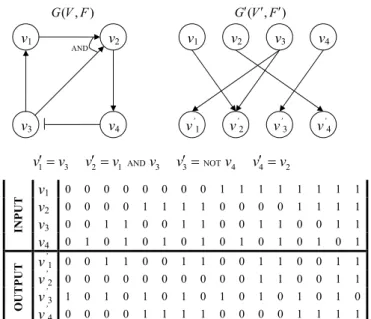
For convenience, we converted the classical Boolean network G(V, F) to the wiring diagram G0_(V0_{, F}0_{) (See Fig. 1) [31]. For each node v}

i∈ V , suppose vi1, vi2, . . . ,

vik are the input nodes assigned to vi. Then we construct an additional node v0iand connected the edge from vij to v0ifor each 1 ≤ j ≤ k. That is, the set of {v1, . . . , vn} represents the gene expression profile at time t and the set of {v0

1, . . . , v0n} corre-sponds to the gene expression profile at time t + 1. Hence we can treat the set

( , ) G V F G V( ,F) AND NOT 1 3 2 1 3 3 4 4 2 v _!v v _!v v v _! v v _!v v₁ 0 0 0 0 0 0 0 0 1 1 1 1 1 1 1 1 v₂ 0 0 0 0 1 1 1 1 0 0 0 0 1 1 1 1 v₃ 0 0 1 1 0 0 1 1 0 0 1 1 0 0 1 1 I N P U T v₄ 0 1 0 1 0 1 0 1 0 1 0 1 0 1 0 1 v’₁ 0 0 1 1 0 0 1 1 0 0 1 1 0 0 1 1 v’₂ 0 0 0 0 0 0 0 0 0 0 1 1 0 0 1 1 v’₃ 1 0 1 0 1 0 1 0 1 0 1 0 1 0 1 0 O U T P U T v’₄ 0 0 0 0 1 1 1 1 0 0 0 0 1 1 1 1 v₁ v₂ v₃ v₄ AND v₁ v₃ v’ 1 v₂ v₄ v’ 2 v ’ 3 v ’ 4

Fig. 1 A Boolean network G(V, F), its wiring diagram G0_(V0_{, F}0_{) and the functional dependency} table

of {v1, . . . , vn} as the input values and the set of {v01, . . . , v0n} as the correspond-ing output values. Therefore, the output values of {v0

1, . . . , v0n} are determined by v0

i= fi(vi1, . . . , vik).

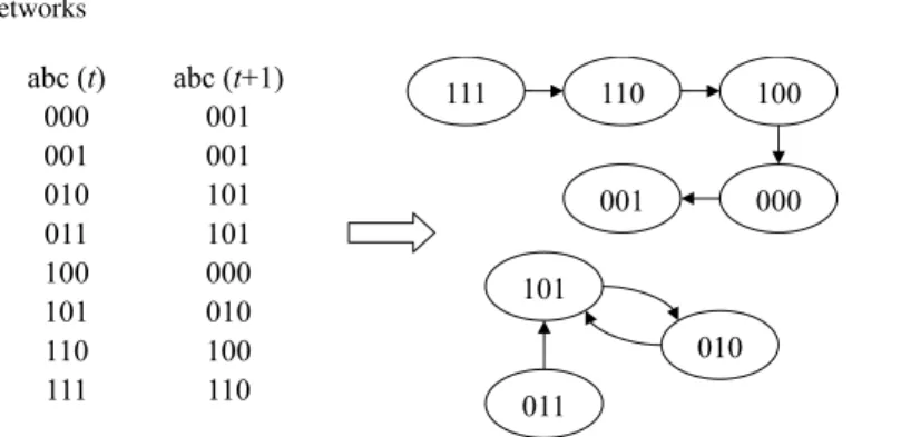
In classical Boolean networks, the states of nodes at time t + 1 depend on the states of nodes at time t, so that all nodes progress synchronously. Usually, in clas-sical Boolean networks, the dynamics of the states of nodes are evolving according to the model structure and the scheme with an initial state. Hence, if the size of node n is fixed, the state space is finite (2n_{). Therefore, given a particular set of} nodes with the corresponding Boolean function, the trajectory or the state transition can be calculated. Consequently, a state will be eventually recur in the Boolean net-work. Since classical Boolean networks are completely deterministic, the dynamics are deterministic and a trajectory must reach a repeating state cycle. This means that the system of the network ultimately transits into an attractor. If an attractor consists of only a single state, it is called a point attractor or a steady state. If an attractor consists of two or more states, it is called a cycle attractor or a state cycle. The set of states that flow towards the same attractor state is called the basin of the attractor [38]. The effects of feedback for Boolean networks have been discussed in [32]. An example of a Boolean network with n = 3 is shown in Fig. 2.

Suppose there is a Boolean network G(V, F) with n nodes v1, v2, . . . , vnand initial joint probability distributions D(v), v ∈ {0, 1}n_{. The joint probability of node in the} next time step would be

abc (t) abc (t+1) 000 001 001 001 010 101 011 101 100 000 101 010 110 100 111 110 111 110 100 000 001 011 101 010

Fig. 2 The gene expression in time t and time t+1 is showed in the left, the transition space are showed in the right. There is one point attractor (001) with four states flowing into it, (111), (110), (100) and (001). There is also one cycle attractor of period two (101↔010), with one states flowing into it, (011)

Pr{ f1(v) = i1, f2(v) = i2, . . . , fn(v) = in} =

∑

j(v)=ij, j=1,...,n

D(v) (1)

The computing procedure could be iterative and the joint probability distribution in time step t could be described as Dt(v) =Ψ(Dt−1(v)) where the mappingΨ is denoted by (1) and Dt−1_{(v) is the joint probability distribution at time t − 1.} There-fore, the joint probability distribution at any time step t would be Dt_{(v) =Ψ}t_(D0_(v))

where D0_{(v) is the initial joint probability distribution.}

If we try to consider all possible networks, there will be 22k

possible functions for each node. In addition, each node has n!/(n − k)! possible ordered combinations for k different links. Therefore, for each target gene, there are 22k

· n!/(n − k)! possible input combinations to constitute a network. Hence, the number of possible networks with n nodes and k input links is the following [7]

( 22

k

n! (n − k)!)

n_.

2.2 Reconstruction of genetic Boolean networks

Here we will discuss the network reconstruction problem with a Boolean network model. Let (Ij, Oj) be the pair of expression profiles for {v1, . . . , vn}, where Ijis the expression at time t and Ojcorresponds to the expression at time t + 1. The network reconstruction problem is to reconstruct the classical Boolean network from a series of pair examples, EX = {(I1, O1), (I2, O2), . . . , (Im, Om)}.

There are a variety of algorithms proposed for reconstructing the structure of a genetic regulatory network from expression data of genes under the model of classi-cal Boolean networks [2, 19]. In this subsection, we will discuss one reconstruction

algorithm called REVEAL proposed in [21]. First, we only consider Boolean net-works in which the indegree of each node is bounded by a constant K, because it has been proven that the number of profiles required grows exponentially if k is not bounded [1]. For simplicity, we only show algorithms for the case of K = 2. However, the algorithm can be intuitively generalized to any K.

We start by computing the Shannon entropy that measures the systematic mutual information of the Boolean network state transition table in the algorithm [26]. The Shannon entropy is defined in term of the probability of an event Piby

H = −

∑

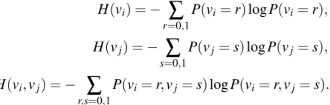
For a pair of binary elements (vi, vj), the individual and combined Shannon en-tropies are defined as

H(vi) = −

∑

∑

∑

One example of a binary system for explaining the calculation of Shannon en-tropy is demonstrated in Fig. 3.

vi 0 1 1 0 0 0 1 1 0 1 vj 0 0 1 0 1 0 1 1 0 0 vi/vj 0 1 0 0.4 0.1 0.5 1 0.2 0.3 0.5 0.6 0.4 ( ) 0.5 log(0.5) 0.5 log(0.5) 1, ( ) 0.6 log(0.6) 0.4 log(0.4) 0.97, ( , ) 0.4 log(0.4) 0.1log(0.1) 0.2 log(0.2) 0.3log(0.3) 1.85. i j i j H v H v H v v ! ! ! ! ! ! ! !

Fig. 3 Calculation of Shannon entropy for single element and pair elements. Probability is calcu-lated by the frequency the state of on or off

The conditional entropy H(vi|vj) corresponds to the information contained in vi but not shared with vj. It can be shown that H(vi, vj) = H(vj) + H(vi|vj). If H(vi, vj) = H(vj), i.e. H(vi|vj) = 0, then all information contained in vi is shared with vjand we would think vjcan determine the expression of vicompletely. Next, we list and demonstrate the procedure of algorithm, REVEAL, for the problem of network reconstruction.

• Step 1: Calculation of entropies from input

We calculate the entropy of every input node {vi}, i = 1, . . . , n. Since the indegree of each node is bounded by K = 2, we also need to calculate the entropies of each pair of input node {vi, vj}, i, j = 1, . . . , n.

• Step 2: Identification of k=1 links For each node v0

i∈ V, i = 1, . . . , n, we calculate the entropies of all single input-output pairs H(v0

i, vj), i, j = 1, . . . , n. If H(v0i, vj) = H(vj), then vjcompletely de-termines v0

i. If there is no single input vj such that H(v0i, vj) = H(vj), execute Step 3, otherwise output vjand constitute the rule between v0iand vj.

• Step 3: Identification of k=2 links For each node v0

i∈ V, i = 1, . . . , n, we calculate the entropies of all pair inputs with one output H(v0

i, vj, vl), i, j, l = 1, . . . , n. If H(v0i, vj, vl) = H(vj, vl), then the pair input (vj, vl) exactly determines v0i. Then we constitute the rule between v0i and vj, vl.

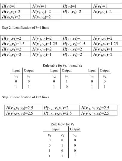
The advantage of this algorithm is its low time and memory complexity. We consider the example by the input/output pairs data as shown in Fig. 1. It is easy to reconstruct the classical Boolean network from the data {(I1, O1), (I2, O2), . . . ,

(I16, O16)} by the algorithm REVEAL. We list the step-by-step demonstration in

Fig. 4 from the network example of Fig.1.

2.3 Analysis of the computational complexity and required number

of experiments

For the network reconstruction problem, we assess the time complexity of the RE-VEAL algorithm. If a node is controlled with exactly k input variables, there are¡n_k¢ possible combinations of input nodes. For the calculation of input entropies with in-degree that is bounded by K, there are¡n₁¢+¡n₂¢+ · · · +¡_Kn¢input entropies that need to be evaluated. This constitute the computational complexity of O(nK_{). Moreover,} for each node, there are¡n_k¢entropies to be calculated in every step of the identifi-cation of k links. In total, there are K steps of identifiidentifi-cation because the indegree is bounded by K. Consequently, for each node,¡n₁¢+¡n₂¢+· · ·+¡_Kn¢entropies are eval-uated in the step of identification with k = 1, 2, . . . , K. Therefore, O(nK+1_{) entropies} are evaluated in total and the REVEAL algorithm works in polynomial time for fixed K. Besides, it has been shown that the O(log n) transition (INPUT/OUTPUT) pairs are necessary and sufficient for the network reconstruction with high probability if the maximum indegree of Boolean networks is bounded [2].

Step 1. Input entropies

H(v1)=1 H(v2)=1 H(v3)=1 H(v4)=1

H(v1,v2)=2 H(v1,v3)=2 H(v1,v4)=2 H(v2,v3)=2

H(v2,v4)=2 H(v3,v4)=2

Step 2. Identification of k=1 links

H(v’ 1,v1)=2 H(v ’ 1,v2)=2 H(v ’ 1,v3)=1 H(v ’ 1,v4)=2 H(v’ 2,v1)=1.5 H(v ’ 2,v2)=1.25 H(v ’ 2,v3)=1.5 H(v ’ 2,v4)=1.25 H(v’ 3,v1)=2 H(v ’ 3,v2)=2 H(v ’ 3,v3)=2 H(v ’ 3,v4)=1 H(v’ 4,v1)=2 H(v ’ 4,v2)=1 H(v ’ 4,v3)=2 H(v ’ 4,v4)=2

Rule table for v_{1, v3and}v₄

Input Output Input Output Input Output

v₃ v₁ v₄ v₃ v₂ v₄

0 0 0 1 0 0

1 1 1 0 1 1

Step 3. Identification of k=2 links

H(v’ 2,v1,v2)=2.5 H(v ’ 2, v1,v3)=2 H(v ’ 2, v1,v4)=2.5 H(v’ 2,v2,v3)=2.5 H(v ’ 2, v2,v4)=2.5 H(v ’ 2, v3,v4)=2.5

Rule table for v₂

Input Output v₁ v₃ v₂ 0 0 0 0 1 0 1 0 0 1 1 1

Fig. 4 The step-by-step demonstration of the algorithm REVEAL for network example showed in Fig. 1

3 Probabilistic Boolean networks

In the previous section, we have introduced the definition and properties of classical Boolean networks. However, the structure of classical Boolean networks has been criticized for its deterministic formality. If the state of every node is obtained at any one time step, the states of all nodes at next time step are determined and fixed in a classical Boolean network model. However, there may be scenarios in which a set of different Boolean functions is required to describe a transition between a set of variables. In this section, we are going to introduce the basic definition and notation

for probabilistic Boolean networks which allow more than one possible Boolean function for each node and extend the network structure to a probabilistic setting.

3.1 Definition and notation

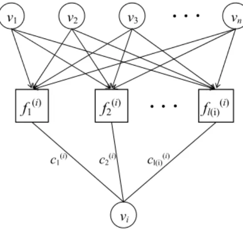
Probabilistic Boolean networks were proposed in [27] as a generalization of the classical Boolean networks with more flexibility due to its non-deterministic struc-ture. In a probabilistic Boolean network, every node vi is assigned by a set Fi= { f₁(i), . . . f_l(i)(i)}, where each f_j(i): {0, 1}n_{→ {0, 1} is a possible Boolean function} de-termining the value of gene vi. Clearly, a probabilistic Boolean network becomes a classical Boolean network if there is only one possible Boolean function for every node vi, that is, the value of l(i)is 1, for all i = 1, . . . , n.

c1(i) v1 v2 v3 vn f1 (i) f2 (i) fl(i) (i) vi

c2(i) cl(i)(i)

Fig. 5 The basic building block for the expression of gene viin a probabilistic Boolean model

We will also refer to the function f(i)_j as a predictor which is one of the possible Boolean function assigned to the expression of gene vi. For every node vi in V , one of the predictors in Fiwould be selected randomly by a predefined probability distribution at any given time step. Therefore, at a given instant of time, a realization of a probabilistic Boolean network is determined by a vector of Boolean functions. We illustrate the basic building block for the expression of gene viof a probabilistic Boolean network in Fig. 5.

Suppose in total there are N different realizations in a probabilistic Boolean net-work, the N vector functions, f1, f2, . . . , fNare defined as fm= ( fm(1)1, f

(2)

m2, . . . , f

(n)

mn),

where 1 ≤ mi≤ l(i)and fm(i)i ∈ Fi(i = 1, 2, . . . , n), for m = 1, 2, . . . , N. Each vector

proba-bilistic Boolean networks. Hence, if the values of all genes (v1, v2, . . . , vn) is known at time t and the realization fm is chosen, fm(v1, v2, . . . , vn) = (v01, v02, . . . , v0n) gives us the state of the genes at time t + 1.

If the predictor for each gene is chosen independently, that is, Pr{ f(i)= fm(i)i, f( j)= f ( j) mj} = Pr{ f(i)= f (i) mi}Pr{ f( j)= f ( j) mj},

for all i, j, mi, mj with 1 ≤ mi≤ l(i), 1 ≤ mj≤ l( j), then the probabilistic Boolean

network is said to be pairwise independent. Under the assumption of independence of the random variables f(1)_{, f}(2)_{, . . . , f}(n)_{, the number of possible probabilistic}

Boolean network realizations is N =

_∏

l(i) [27].

Although the domain of each predictor function f(i)_j is {0, 1}n_{, there should be} many fictitious variables that are not needed in the function. A variable vi is de-scribed as fictitious for a function f , if the state of viwould not affect the output of function f , that is,

f (v1, . . . , vi−1, 0, vi+1, . . . , vn) = f (v1, . . . , vi−1, 1, vi+1, . . . , vn) (2) for all v1, . . . , vi−1, vi+1, . . . , vn. Consequently, there are only a few input genes that actually regulate gene xiat any given time. Let f be a random vector, representing the realization of a probabilistic Boolean network, then f = ( f(1)_{, f}(2)_{, . . . , f}(n)_),

where f(i)∈ Fifor all i = 1, 2, . . . , n. Hence, for a node vi, the probability that f(i)j is selected as the predictor (1 ≤ j ≤ l(i)) is

c(i)_j = P( f(i)_{= f}(i)

j ) =

∑

m: f_mi(i)= f(i)_j

Pr{ f = fm} (3)

If we define the N × n matrix M as

M =                    1 1 · · · 1 1 1 1 · · · 1 2 .. . ... . .. ... ... 1 1 · · · 1 l(n) 1 1 · · · 2 1 1 1 · · · 2 2 .. . ... . .. ... ... 1 1 · · · 2 l(n) .. . ... . .. ... ... l(1) l(2) · · · l(n − 1) l(n)                    .

each one corresponding to a possible network configuration, then the probability of network i being selected is

Pi= Pr{Network i is selected} = n

∏

c( j)_{Mi j}, (4)

where Mi jis the i jth entry in matrix M.

Next, we establish a 2n_{× 2}n_{state transition matrix A by} A(v, v0) = Pr{(v1, . . . , vn) → (v01, . . . , v0n)} =

_∑

It was shown that the state transition matrix A is a Markov matrix and the proba-bilistic Boolean network is a homogeneous Markov process [27].

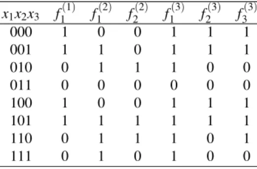
Let us illustrate the above construction with an example. We consider a proba-bilistic Boolean network consisting of three genes V = {v1, v2, v3} and the function

sets F = {F1, F2, F3} with F1= { f1(1)}, F2= { f1(2), f (2) 2 }, F3= { f1(3), f (3) 2 , f (3) 3 }. The

rule of each function is given by the following truth table.

Table 1 One example of probabilistic Boolean network model

x1x2x3 f₁(1) f₁(2) f₂(2) f₁(3) f₂(3) f₃(3) 000 1 0 0 1 1 1 001 1 1 0 1 1 1 010 0 1 1 1 0 0 011 0 0 0 0 0 0 100 1 0 0 1 1 1 101 1 1 1 1 1 1 110 0 1 1 1 0 1 111 0 1 0 1 0 0

By assuming the independence of the probabilistic Boolean network, there are 6 possible realizations in this example and the matrix M becomes

M =         1 1 1 1 1 2 1 1 3 1 2 1 1 2 2 1 2 3         .

The network i represented by the ith row of M is selected meaning that the predictors ( f_M(1)_i1, f_M(2)_i2, f_M(3)_i3) will be used.

Let Pi be the probability that network i is selected. In this example, the state transition matrix A is given by

A =             0 0 0 0 0 1 0 0 0 0 0 0 0 P4+ P5+ P60 P1+ P2+ P3 0 0 P2+ P3+ P5+ P6 P1+ P4 0 0 0 0 1 0 0 0 0 0 0 0 0 0 0 0 0 1 0 0 0 0 0 0 0 0 0 1 0 0 P2+ P5 P1+ P3+ P4+ P60 0 0 0 P5+ P6P4 P2+ P3 P1 0 0 0 0             .

3.2 Inference of probabilistic Boolean networks

For a given gene, there is a set of predictors that could be selected. One approach to estimate the probability is the method of coefficient of determination (COD) which was used in an optimal nonlinear filter design [5, 18]. Let v1be a target gene that we

wish to predict by a set of predictors function f₁(i), f₂(i), . . . , f_l(i)(i). For each predictor f(i)_j , one can use the COD to find a set of genes v(i)_j such that f_j(i)(v(i)_j ) are the optimal predictors.

Specifically, the CODs for virelated to the predictor f(i)_j (v(i)_j ) for each j is defined as

θi_j=εi−ε(vi, f

(i)

j (v(i)j ))

εi ,

whereεiis the error of the best estimate of viwithout any conditional variables and ε(vi, fj(i)(v(i)j )) is the error measure of vigiven the predictor f(i)j . It is clear that the value of COD is between 0 and 1. The large value of COD indicate higher evidence that the corresponding predictor with its input genes are plausible.

Let us now assume predictors f₁(i), f₂(i), . . . , f_l(i)(i) with a class of gene sets v(i)₁ , v(i)₂ , . . . , v(i)_l(i) are selected with the highest CODs. Then, for a given gene vi, the probability that predictor f(i)_j is selected is estimated by

C(i)_j = θ i j l(i)

∑

The number of predictors, l(i), is a parameter selected by the user based on the amount of training data available and existing biological information.

3.3 Influences between pairs of genes in probabilistic Boolean

networks

In the probabilistic Boolean network model, every gene is influenced by a set of Boolean functions with several input genes. However, the contribution of every input gene is not always the same. Hence, it is important to distinguish genes that have major impacts on the predictor from those that have minor impacts.

Since every gene is controlled by a set of Boolean functions, we first consider the influence of variables on a Boolean function. One method is to quantify the influence of a variable on a Boolean function, as proposed in [27, 29]. The influence of the variable vjon the function f is defined as

Ij( f ) = ED[_∂∂_vf

j] = Pr{ f (v) 6= f (v

( j)_)}

where ED[ ] is the expectation operator with respect to distribution D(v) and v( j) is the same as v with jth component is toggled (from 0 to 1, or from 1 to 0). For a probabilistic Boolean network, Fi denotes the set of predictor for gene vi with corresponding probabilities c(i)₁ , . . . , c(i)_l(i). Hence, the influence of gene vmon gene vi can be defined as Im(vi) = l(i)

∑

where Im( f(i)j ) is the influence of variable xm on the predictor f(i)j . The influence matrixΓ with elements ofΓi j= Ii(vj) collects the information of influence between every pair of genes.

We consider the probabilistic Boolean network shown in Table 1 with c(1)₁ = 1, c(2)₁ = 0.4, c(2)₂ = 0.6, c(3)₁ = 0.2, c(3)₂ = 0.4, c(3)₃ = 0.4. We let the initial joint probability distribution D be an uniform distribution, that is, D(v) = 1/8 for all v ∈ [0, 1]3_{. Suppose we would like to compute the influence of variable v}

1on variable

I1( f1(2)) = ED[ ∂f₁(2)(v) ∂v1 ] = 0.25, I1( f2(2)) = ED[∂f (2) 2 (v) ∂v1 ] = 0.25.

Hence, the influence of variable v1on variable v2would be

I1(v2) = I1( f1(2)) · c(2)1 + I1( f2(2)) · c(2)2 = 0.4 · 0.25 + 0.6 · 0.25 = 0.25.

By computing every pair of gene similar to the process above, we can obtain the influence matrix Γ =  0 0.25 0.15_{1 0.75 0.75} 0 0.75 0.15   .

4 Directed acyclic Boolean networks

In the previous section, we introduced the classical Boolean network model and the probabilistic Boolean network model in order to analyze the expression profiles of genes with time courses. However, in some experiments, the expressions of genes only can be observed at a specific time. Therefore, in this section, we will discuss a directed acyclic Boolean network model for handling the static and dynamic expres-sion profiles of genes [20]. A directed acyclic Boolean network is uniquely deter-mined by the state space of its elements: all possible on-off states that are compat-ible with the network structure. Our goal is to reconstruct directed acyclic Boolean networks from possibly noisy array data.

4.1 The structure of directed acyclic Boolean networks

Firstly, we will introduce the structure of directed acyclic Boolean networks. Sup-pose there are m elements, v1, v2, . . . , vmin a Boolean network. For any two elements viand vj, we have two kinds of pairwise relationships: prerequisite and similarity. We say that viis prerequisite for vjif the on-status of viis necessary for the on-status of vjand this relationship is denoted by vi≺ vj. That is, if we know the status of vj is 1 and vi≺ vj, then the status of vimust be 1. Therefore for any pair of elements (vi, vj) with a prerequisite relation, there are a total of four possible relationships: vi≺ vj, vi≺ ¯vj, ¯vi≺ vjand ¯vi≺ ¯vj. The prerequisite relationship is transitive, thus if vi≺ vjand vj≺ vk, then we have vi≺ vk. For any pair of elements (vi, vj) which

have prerequisite relationship vi≺ vj, we say they are covering pair if there are no other element vksuch that vi≺ vkand vk≺ vj.

The other types of relationships between pairs of elements is similarity and neg-ative similarity. We say that vi and vj are similar if the status of two elements is consistent. That is, the status of these two elements is on and off simultaneously, and this is denoted by vi∼ vj. There is another relationship of negative similarity and there are two possible relationships: vi∼ vjand vi∼ ¯vj.

In the diagram, if vi is prerequisite to vj, we draw a directed arrow from the vertex vito vj, and if viis similar to vj, we use an undirected line to connect viand vj. For the purpose of making the prerequisite relationships more clear in the graph, we only represented all partial orders by arrows between covering pairs.

v4

v1

v2 v3

v5

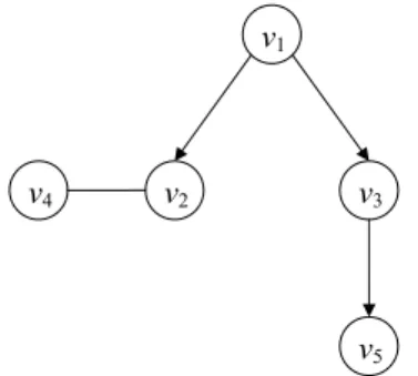
Fig. 6 A diagram of directed acyclic Boolean network with the corresponding table of states

We will illustrate the above construction by an example with Fig. 6 which has five elements with one similarity and four prerequisite relationship. For five Boolean elements, there are totally 25_{= 32 possibilities in the state space and only 7 states}

are compatible with the diagram.

Table 2 The table of states for directed acyclic Boolean network shown in Fig. 6

Case 1 2 3 4 5 6 7 v1 0 1 1 1 1 1 1 v2 0 0 0 0 1 1 1 v3 0 0 1 1 0 1 1 v4 0 0 0 0 1 1 1 v5 0 0 0 0 0 0 1

The 7 states that are compatible with Fig. 6 are enumerated in Table 2. Sup-pose we generate n samples from the directed acyclic Boolean network in Fig. 6. That is, we sample with replacement from Table 2 and arrange the data in a

ma-trix (yi j), where i = 1, . . . , n, j = 1, . . . , 5. We can identify the relationship of each pair of elements as prerequisite or as similar relationships from the corresponding two columns of data matrix (yi j), which is the transposition of Table 2. Then, the directed acyclic Boolean network would be reconstructed by integrating the pair relationships together. For each pair of elements, we count the frequencies in four cells of (vi, vj) for (0, 0), (0, 1), (1, 0), (1, 1) from the samples and arrange them in a 2 × 2 table. We mark a cell ” + ” if the frequency count is positive and mark it ”0” otherwise. Then, we check the table with those six pairwise relationships listed in Table 3. For example, if we consider the paired elements v1and v2, the frequency

counts of (v1, v2) for (0, 0), (1, 0) and (1, 1) are positive and there is no incident for

(0, 1), therefore, the relationship between v1and v2would be v1≺ v2.

Table 3 Count patterns for the basic six relationships assuming exhaustive sampling and no mea-surement error vi∼ vj vi≺ ¯vj ¯vi≺ vj vi/vj 0 1 vi/vj 0 1 vi/vj 0 1 0 + 0 0 0 + 0 + + 1 0 + 1 + + 1 + 0 vi∼ ¯vj vi≺ vj ¯vi≺ ¯vj vi/vj 0 1 vi/vj 0 1 vi/vj 0 1 0 0 + 0 + 0 0 + + 1 + 0 1 + + 1 0 +

4.2 Identification algorithm with noisy array

In subsection 4.1, we discussed an identification method for data without noise. In this subsection we will consider the situation of noisy array data. We assume that every element in the entry of (yi j), j = 1, 2, . . . , m switches to its reverse status with a misclassification probability p independently; that is

xi j= ½

yi j with probability 1 − p;

1 − yi jwith probability p. (6)

Thus, the observed array (xi j) contains misclassification error. Our goal is to recon-struct directed acyclic Boolean networks from noisy array of binary data (xi j).

In the first step, we investigate every pair of elements for possible relationships. Next, we use the probabilistic model of equation (6) to estimate misclassification probability p. We treat the data in the 2 × 2 table as a multinomial distribution with

four cells whose probabilities are q00, q01, q10, q11, respectively, where q00+ q01+

q10+ q11= 1.

The observed data n00, n01, n10, n11are generated from the multinomial

distribu-tion with probability r00, r01, r10, r11, where r00+ r01+ r10+ r11= 1. The

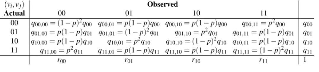
relation-ship between qi jand ri jis displayed in Table 5 and explained below.

Table 4 Splitting counts caused by misclassification error

(vi, vj) Observed Actual 00 01 10 11 00 m00,00 m00,01 m00,10 m00,11 m00 01 m01,00 m01,01 m01,10 m01,11 m01 10 m10,00 m10,01 m10,10 m10,11 m10 11 m11,00 m11,01 m11,10 m11,11 m11 n00 n01 n10 n11 n

Table 5 Splitting probabilities caused by the misclassification error

(vi, vj) Observed Actual 00 01 10 11 00 q00,00= (1 − p)2q00 q00,01= p(1 − p)q00 q00,10= p(1 − p)q00 q00,11= p2q00 q00 01 q01,00= p(1 − p)q01 q01,01= (1 − p)2q01 q01,10= p2q01 q01,11= p(1 − p)q01 q01 10 q10,00= p(1 − p)q10 q10,01= p2q10 q10,10= (1 − p)2q10 q10,11= p(1 − p)q10 q10 11 q11,00= p2q11 q11,01= p(1 − p)q11 q11,10= p(1 − p)q11 q11,11= (1 − p)2q11 q11 r00 r01 r10 r11 1

Because of the misclassification error, a portion of samples of m00may change to

the other three cells. We use the notations of m00,00, m00,01, m00,10, m00,11to represent

the counts of four cells changed from m00. Analogous notations are defined for

m01, m10and m11. Consequently, their generating probabilities (q00, q01, q10, q11) are

calculated as follows: qi j,kl= p|i−k|+| j−l|(1 − p)2−|i−k|−| j−l|qi j. Here, we adopt the notation qi j,kl analogous to mi j,kl. The above parameters and splits are shown in Table 4 and Table 5. By these two table, it is easy to find that the correspondence between two sets of counts and probabilities is the following:

     nkl=

∑

∑

     mi j=

∑

∑

For the complete data {mi j,kl}, the log-likelihood is given by

L =

_∑

i, j,k,l=0,1

mi j,kllog qi j,kl, (8)

where qi j,kl are those splitting probabilities. Since the complete data {mi j,kl} are not observable, we use the M algorithm to maximize the log-likelihood. In the E-step, the splitting counts of complete data {mi j,kl} are evaluated by the conditional expectations using the current values of the parameters by the following formula

Ep,q00,q01,q10,q11(mi j,kl|nkl) =

nklqi j,kl

∑

qi0_j0_,kl, (9)

where i, j, k, l = 0, 1. One or two probabilities of q00, q01, q10, q11are zero in those

different hypotheses specified in Table 6. In the M-step, we maximize the condi-tional expectation of the log-likelihood for the complete data to obtain the maxi-mum likelihood estimates (MLEs) of the parameters. According to the MLEs, we can compute the p-score or s-score for every pair of elements, which are obtained by the estimate for the misclassification probability under prerequisite or similar relationship.

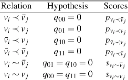
Table 6 The six basic relationships and their corresponding probabilistic hypotheses and scores

Relation Hypothesis Scores vi≺ ¯vj q00= 0 pvi≺ ¯vj vi≺ vj q01= 0 pvi≺vj ¯vi≺ vj q10= 0 p¯vi≺vj ¯vi≺ ¯vj q11= 0 p¯vi≺ ¯vj vi∼ ¯vj q01= q10= 0 svi∼ ¯vj vi∼ vj q00= q11= 0 svi∼vj

For the first step, we would like to determine the most probable relationships between elements and select candidate pairs of genes for the watch list. Next, we reconstruct a directed acyclic Boolean network by integrating the relationship of those genes selected.

For a pair of genes viand vj, we define the p-scores pvi≺ ¯vj, pvi≺vj, p¯vi≺ ¯vj, p¯vi≺vj

are, respectively, the maximum likelihood estimates of p under the triangular model: q00= 0, q01= 0, q10= 0, q11= 0. The s-scores svi∼vj and svi∼ ¯vj are the maximum

likelihood estimates of p under the diagonal model: q01= q10= 0 and q00= q11= 0,

respectively.

According to the E-M algorithm described above, we can evaluate the s-score and p-score for every pair of elements. We use the MLE ˆp to measure how well each hypothesis fits: the smaller the score, the more evidence that the corresponding hypothesis could be true.

For each pair of elements, we find the diagonal model which have the smaller s-score and the triangular model which have the smallest p-score. Then we evaluate their BIC values by

BIC = − log likelihood +d log n

2 ,

where d is the number of parameters for one possible relationship. We treat the model with the smaller BIC value as the most probable relationship for the pair elements and the s-p-score is defined as the corresponding score under the model. Next, for every pair of elements, we rank its s-p-score in the ascending order. The smaller the s-p-score is, the more likely the relationship could be true.

If the samples are generated from a directed acyclic Boolean network, s-p-scores are quite useful for the discovery of pairwise relationships. Here we could consider the maximum compatibility criterion: to choose the maximum threshold value so that the selected relationships contain no conflicts [20]. We collect those relation-ships whose s-p-scores are smaller than a threshold. Known biological results could be helpful for the determination of a threshold. For example, if we know the re-lationshp v1≺ v3is true, then the s-p-scores smaller than pv1≺v3 should be in our

watch list. As more relationships are included in the watch list, the more likely we are to observe incompatible ones. In general, we can choose the threshold which allows the maximum number of relationships with no conflicting relationships.

We now evaluate the computational complexity of statistical reconstruction method of SPAN described above. The key procedure is the computation of s-p-score for every pair of elements. If the number of elements is m, their are totally ¡_m

2

¢

pairs of elements and the complexity for the computation of MLE is O(m2_{). We}

can rank the s-p-score of every pair elements in the order of O(m2_{log m). Thus, in}

this statistical reconstruction algorithm, the time complexity is O(m2_{log m) and the}

memory complexity is O(m2_{) as described in [20].}

5 Conclusion

We have introduced a variety of models including classical Boolean networks, prob-abilistic Boolean networks and directed acyclic Boolean networks for dealing with genetic regulatory networks. These variants of Boolean networks can be used in the exploration of large genetic networks because of the simple structure of Boolean networks. Based on the reconstruction of Boolean networks, more flexible models, like Bayesian networks, can be applied to investigate more complex problems.

There are several advantages in estimating gene regulatory networks with Boolean networks. First of all, a variety of software packages have recently been developed for constructing Boolean networks. Matlab implementations of classical Boolean network toolbox and for probabilistic Boolean networks were developed in [25] and [27]. Moreover, Li and Lu also provided an implementation for the s-p-scoring method in Matlab [20]. Other genetic regulatory network tools such as NetBuilder for simulating genetic Boolean network are also available [24]. Second, recent re-search indicates that various complex biological processes can be described by seemingly simplistic Boolean formalisms [34, 35]. The dynamic behaviors of living systems can be explained effectively by Boolean networks [9, 30]. Moreover, for large-scale gene regulatory networks, Kim et al. [17] have used Boolean network with chi-square test on the yeast cell cycle microarray gene expression data sets. Kauffman et al. [16] have used a random Boolean network to get possible inter-action rules for transcriptional network models in yeast. Furthermore, the dynamic behaviors of cellular states are also represented by attractors in Boolean network in [9].

One characteristic of a Boolean network is that all the variables in the graph are binary. If the data we observed is continuous or quantized to have more than two levels, we need to discretize them. For microarray data, the ratios of expression level would be one possible approach of discretization. That is, we can treat the gene as on (active) if the log-ratio of its expression is larger than zero and off (inactive) otherwise. In general, biological background knowledge will be helpful for setting thresholds for discretizaion. On the other hand, if the samples are obtained from a time course, then we can consider the gene as on or off by detecting the gene is either increasing or decreasing with time.

For future developments on Boolean networks, we can consider more compli-cated structures such as Boolean networks with time delay. Furthermore, we can develop models of Boolean networks that have more flexible structures than these models proposed in literature. Since Boolean network models have been shown to be useful for reconstructing genetic network from real biological gene expression profiles, the evaluation of Boolean network models’ effectiveness will be an impor-tant task in the future.

Acknowledgements The authors would like to express their gratitude to the English editing of Yang Wang and Arthur Tu. This research was partially supported by the National Science Council, National Center for Theoretical Sciences and Center of Mathematical Modeling and Scientific Computing (CMMSC) at the National Chiao Tung University in Taiwan.

References

[1] Akutsu, T., Kuhara, S., Maruyama, O., Miyano, S.: Identification of gene reg-ulatory networks by strategic gene disruptions and gene overexpression. Proc.

9th ACM-SIAM Symp. Discrete Algorithms pp. 695–702 (1998)

[2] Akutsu, T., Miyano, S.: Identification of genetic networks from a small num-ber of gene expression patterns under the Boolean network model. Pacific Symposium on Biocomputing 4, 17–28 (1999)

[3] Akutsu, T., Miyano, S., Kuhara, S.: Inferring qualitative relations genetic net-works and metabolic pathways. Bioinformatics 16, 727–734 (2000)

[4] Bornholdt, S.: Less is more in modeling large genetic networks. Science 310(5747), 449–451 (2005)

[5] Dougherty, E.R., Kim, S., Chen, Y.: Coefficient of determination in nonlinear signal processing. Signal Processing 80, 2219–2235 (2000)

[6] Friedman, N., Linial, M., Nachman, I., Pe’er, D.: Using Bayesian networks to analyze expression data. Journal of Computational Biology 7, 601–620 (2000) [7] Harvey, I., Bossomaier, T.: Time out of joint: attractors in asynchronous ran-dom Boolean network. Proceedings of the Fourth European Conference on Artificial Life pp. 67–75 (1997)

[8] Heckerman, D., Geiger, D., Chickering, D.M.: Learning Bayesian networks: the combination of knowledge and statistical data. Machine Learning 20, 197– 243 (1995)

[9] Huang, S.: Gene expression profiling, genetic networks and cellular states: An integrating concept for tumorigenesis and drug discovery. Journal of Molecu-lar Medicine 77, 469–480 (1999)

[10] Imoto, S., Goto, T., Miyano, S.: Estimation of genetic networks and functional structures between genes by using Bayesian network and nonparametric re-gression. Pacific Symposium on Biocomputing 7, 175–186 (2002)

[11] Imoto, S., Higuchi, T., Goto, T., Tashiro, K., Kuhara, S., Miyano, S.: Combin-ing microarrays and biological knowledge for estimatCombin-ing gene networks via Bayesian networks. Journal of Bioinformatics and Computational Biology 2, 77–98 (2004)

[12] Jensen, F.V.: An introduction to Bayesian networks. University College Lon-don Press, LonLon-don (1996)

[13] Jensen, F.V.: Bayesian networks and decision graphs. Springer, New York (2001)

[14] Kauffman, S.A.: Metabolic stability and epigenesis in randomly constructed genetic nets. Journal of Theoretical Biology 22(3), 437–467 (1969)

[15] Kauffman, S.A.: The Origins of Order: self-organization and selection in evo-lution. Oxford University Press, New York (1993)

[16] Kauffman, S.A., Peterson, C., Samuelsson, B., Troein, C.: Random Boolean network models and the yeast transcriptional network. Biophysics 100(25), 14,796–14,799 (2003)

[17] Kim, H., Lee, J.K., Park, T.: Boolean networks using the chi-square test for inferring large-scale gene regulatory networks. BMC Bioinformatics 8, 37 (2007)

[18] Kim, S., Dougherty, E.R., Chen, Y., Sivakumar, K., Meltzer, P., Trent, J.M., Bittner, M.: Multivariate measurement of gene expression relationships. Ge-nomics 67, 201–209 (2000)

[19] Laubenbacher, R., Stigler, B.: A computational algebra approach to the reverse engineering of gene regulatory networks. Journal of Theoretical Biology 299, 523–537 (2004)

[20] Li, L.M. and Lu, H.H.-S.: Explore biological pathways from noisy array data by directed acyclic Boolean networks. Journal of Computational Biology 12(2), 170–185 (2005)

[21] Liang, S., Fuhrman, S., Somogyi, R.: REVEAL, a general reverse engineering algorithm for inference of genetic network architectures. Pacific Symposium on Biocomputing 3, 18–29 (1998)

[22] Moler, E.J., Radisky, D.C., Mian, I.S.: Integrating naive Bayes models and external knowledge to examine copper and iron homeostasis in S. cerevisiae. Physiol Genomics 4(2), 127–135 (2000)

[23] Pearl, J.: Probabilistic reasoning in intelligent systems: networks of plausible inference. Morgan Kaufmann, San Mateo (1988)

[24] Schilstra, M.J., Bolouri, H.: Modeling the regulation of gene expression in genetic regulatory networks. URL http://strc.herts.ac.uk/bio/ maria/NetBuilder

[25] Schwarzer, C.: Matlab random Boolean network toolbox. Swiss Federal Institute of Technology Lausanne(EPFL) (2003). URL http://www. teuscher.ch/rbntoolbox/

[26] Shannon, C.E., Weaver, W.: The mathematical theory of communication. Uni-versity of Illinois Press (1963)

[27] Shmulevich, I., Dougherty, E.R., Kim, S., Zhang, W.: Probabilistic Boolean networks: a rule-based uncertainty model for gene regulatory networks. Bioin-formatics 18(2), 261–274 (2002)

[28] Shmulevich, I., Dougherty, E.R., Zhang, W.: From Boolean to probabilistic Boolean networks as models of genetic regulatory networks. Proceeding of the IEEE 90(11), 1778–1792 (2002)

[29] Shmulevich, I., Dougherty, E.R., Zhang, W.: Gene perturbation and interven-tion in probabilistic Boolean networks. Bioinformatics 18(10), 1319–1331 (2002)

[30] Shmulevich, I., Gluhovsky, I., Hashimoto, R.F., Dougherty, E.R., Zhang, W.: Steady-state analysis of genetic regulatory networks modelled by probabilistic Boolean networks. Comparative and Functional Genomics 4, 601–608 (2003) [31] Somogyi, R., Sniegoski, C.A.: Modeling the complexity of genetic networks: Understanding multigene and pleiotropic regulation. Complexity 1, 45–63 (1996)

[32] Sontag, E., Veliz-Cuba, A., Laubenbacher, R., Jarrah, A.S.: The effect of nega-tive feedback loops on the dynamics of Boolean networks. Biophysical Journal 95, 518–526 (2008)

[33] Spirtes, P., Glymour, C., Scheines, R.: Causation, prediction and search. MIT Press, Cambridge, MA (2000)

[34] Szallasi, Z., Liang, S.: Modeling the normal and neoplastic cell cycle with ”realistic Boolean genetic networks”: their application for understanding car-cinogenesis and assessing therapeutic strategies. Pacific Symposium on Bio-computing 3, 66–76 (1998)

[35] Thomas, R., Thieffry, D., Kaufman, M.: Dynamical behaviour of biological regulatory networksXI. Biological role of feedback loops and practical use of the concept of the loop-characteristic state. Bulletin of Mathematical Biology 57(2), 247–276 (1995)

[36] Wolfram, S.: Statistical mechanics of cellular automata. Reviews of Modern Physics 55(3), 601–644 (1983)

[37] Wolfram, S.: Universality and complexity in cellular automata. Physica 10D 10(1), 1–35 (1984)

[38] Wuensche, A.: Genomic regulation modeled as a network with basins of at-traction. Pacific Symposium on Biocomputing 3, 89–102 (1998)