國
立
交
通
大
學
資訊學院
資訊工程學系
博
士
論
文
物件追蹤感測網路中與位置管理相關的通訊協定
Communication Protocols for Location Management in Object
Tracking Sensor Networks
研 究 生:林致宇
指導教授:曾煜棋 教授
物件追蹤感測網路中與位置管理相關的通訊協
Communication Protocols for Location Management in Object Tracking Sensor
Networks
研 究 生:林致宇 Student:Chih-Yu Lin
指導教授:曾煜棋 Advisor:Yu-Chee Tseng
共同指導教授:彭文志 Co-advisor:Wen-Chih Peng
國 立 交 通 大 學 資 訊 學 院
資 訊 工 程 學 系
博 士 論 文
A DissertationSubmitted to Department of Computer Science College of Computer Science
National Chiao Tung University in partial Fulfillment of the Requirements
for the Degree of Doctor of Philosophy
in
Computer Science
September 2007
Hsinchu, Taiwan, Republic of China
物件追蹤感測網路中與位置管理相關的通訊協定
學生:林致宇
指導教授
:曾煜棋 教授
彭文志 教授
國立交通大學資訊工程學系﹙研究所﹚博士班
摘
要
無線通訊與感測技術的快速發展使得無線感測網路成為一門新興的科技,無線感測網路的應用 也因此被廣泛地討論。在無線感測網路中物件追蹤是一個重要的議題,它包含了許多的應用, 例如軍事上入侵者的偵測、野生動物棲息地的監控等。物件追蹤包含了幾個重要的步驟,例如 事件的偵測、目標物的辨識、位置的估算等,在無線感測網路中,當物件的位置被估算出來之 後,為了能讓使用者去查詢物件的位置,或者為了能讓感測到物件的感測器做回報,一個位置 管理機制是需要的。本論文的主題即討論無線感測網路上位置管理相關的通訊協定。我們所提 出的位置管理機制利用了無線感測網路的網路內資料處理的能力,以分散式的方式去執行物件 位置的更新與查詢。我們更考量了在多資料匯集端的網路下的位置管理機制,在這樣的環境下 我們假設使用者可在任一個地方發出位置的查詢。而由於感測資料的不精確是感測網路先天上 特有的特性,我們也考慮了在使用者可容忍一些誤差的網路環境下,位置管理機制該如何達成 的問題。而不管在哪一種網路環境下,位置管理機制的目的都是為了要降低位置更新與位置查 詢所產生的通訊成本。此外,我們觀察到網路底層封包的遺失與碰撞可能導致物件追蹤網路中 產生不正確的位置資訊,而物件追蹤網路是一種以事件驅動為主的網路,因此我們也針對以事 件驅動為主的感測網路提出了一個鏈結層通訊協定來降低封包碰撞的問題。 物件追蹤通常包含了兩個基本的操作:位置更新與位置查詢。一般而言,位置更新是在當一個 物件從一個感測區域移動到另一個感測區域時發生,而位置查詢則是當使用者有需要知道物件 的位置而發生查詢。無線感測網路處理位置更新與查詢的方法有很多,一個處理更新與查詢最 簡單的做法是將使用者的查詢送給網路上的每一個感測節點,而偵測到物件的感測器在收到查 詢後就會回覆物件的位置給資料匯集端,我們可以發現在這個方法中,感測器不需要主動地做 位置的更新,然而,很顯然這個方法在網路規模很大或者是查詢頻率很高時會非常地沒有效 率,因為使用者的查詢必須被廣播到整個網路上。第二種處理更新與查詢的方法則是要求感測 器偵測到物件時就必須主動地將物件的新位置傳送給資料匯集端,如此資料匯集端就隨時有物 件的位置資訊,因此資料匯集端本身就可以馬上回覆使用者的查詢,而不再需要將查詢送到感 測網路上,然而這方法在物件移動相當頻繁時會產生許多的位置更新訊息,因此我們可以很明 顯地看出上述兩個方法是各有利弊。在這篇論文中,我們首先針對單一資料匯集端的網路環境 提出一個樹狀的位置管理機制,在建樹的過程中,我們考量了網路實際上的拓樸對通訊代價產 生的影響。建樹的程序主要分成兩個階段,在第一個階段我們主要目的是降低位置更新所產生 的通訊代價,我們利用了避免偏向(deviation-avoidance)與高移動頻率優先(high-weight-first)這 個特性去降低通訊代價。而在第二個階段,我們則是以第一階段所產生的樹再加上位置查詢的
考量而去做調整。 接著,我們則考慮了一個多資料匯集端的感測網路。擁有多重資料匯集端的一個好處是可降低 位置查詢的回應時間,除此之外也能降低資料匯集端附近網路流量擁塞的問題,亦即可達到較 好的負載平衡。為了要支援多資料匯集端的環境,我們可考慮將單一資料匯集端的方法做延 申,也就是每個資料匯集端都建構一個樹,然而這也就意謂著更新多個樹是需要的,因此如何 去降低更新多個樹所產生的通訊代價便是我們要去解決的問題。在這篇論文中,為了解決此問 題,我們利用了資料匯集的概念提出了有效率的位置更新機制。有了這個機制,我們發現在多 重資料匯集端的環境下,位置更新的通訊代價只會增加少許。此外,我們也根據前述的更新機 制推導出更新代價的公式,並以此公式設計出兩個分散式的建樹演算法。 在物件移動的環境中要維持物件正確的位置資訊幾乎是不可能的,原因除了定位技術本身就不 是很準確,物件的移動與資料傳送的延遲也都使得查詢者得到的位置資訊並不精確。然而幸運 的是在物件追蹤的應用中,不精確的位置資訊通常是能夠被容忍的,例如生物科學家為了要追 蹤某動物時,生物學家可能只需要知道大概的移動方向即可而不需要知道正確的位置,除此之 外,當科學家只是為了要觀察動物的日常作息時,幾個小時前的位置資訊對科學家們仍是有用 的資訊。因此我們也提出了一個位置管理機制去支援能夠容忍不精確位置資訊的物件追蹤感測 網路。我們認為這個位置管理機制應該要能達成兩個目標,第一,位置查詢的通訊代價應該跟 精確程度成正比,第二,多精確程度的支援。我們觀察到樹狀架構的位置管理機制可以很容易 地達成這兩個目標,因此我們也提出了一個建樹的演算法。 藉著實驗的模擬我們觀察到封包的碰撞與遺失會導致使用者得到不正確的物件位置資訊,因此 我們也提出了一個鏈結層協定來減輕碰撞的問題。無線感測網路一般可分成兩類,一是事件驅 動另一則是時間驅動。在事件驅動的感測網路中,感測器會在偵測到事件時做回報的動作,而 這樣的回報可能造成事件發生區域的感測器遭受到較高的傳輸競爭。在這篇論文中,我們結合 了兩個議題來解決這個問題,一是利用感測資料的空間相關性,另一則是設計一個新的媒介存 取協定。我們提出了一個結合 TDMA(Time Division Multiple Access)與 CSMA(Carrier Sense Multiple Access)的鏈結層協定,它與傳統以 TDMA 為基礎的協定有幾個不同的特色。第一, 在 TDMA 的部份我們只需要較寬鬆的時間同步且是經由事件的驅動而啟動 TDMA,而 CSMA 則在非事件發生區域被採用以達到低傳送延遲。第二,時槽分配策略考量了感測資料的空間相 關性,我們發現藉著允許一個感測器可使用和其鄰居相同的時槽,可使得整個網路所需要的時 槽數大幅地降低。第三,藉著拉長一個時槽的長度,我們可在封包離開事件區域後能像水流一 樣依序地前進,每個封包會相隔一定的距離以避免干擾。除此之外,利用 TDMA 的特性及感 測資料的空間相關性,我們也提出了一個降低回報量的機制。而為了達到省電的目的,我們也 討論如何將 LPL (Low Power Listening)的技術結合到我們的方法。
關鍵詞:無線感測網路、物件追蹤、網路內資料處理、資料匯集、行動計算、位置管理、媒 介存取控制、空間相關性、TDMA、CSMA
Communication Protocols for Location Management in
Object Tracking Sensor Networks
Student:Chih-Yu Lin
Advisors:Dr. Yu-Chee Tseng
Dr. Wen-Chih Peng
Department of Computer Science
National Chiao Tung University
ABSTRACT
The rapid progress of wireless communication and embedded micro-sensing MEMS
technologies has made wireless sensor networks (WSNs) possible. Applications of WSNs have been studied widely. Object tracking is one of the important issues of WSNs, which has applications in such as military intrusion detection and habitat monitoring. The key steps involved in object tracking include event detection, target classification, and location estimation. In a WSN, when the locations of objects are successfully determined, a location management scheme for reporting objects'
locations and disseminating users' queries is required. The main theme of this dissertation is location management. The proposed location management schemes explore the in-network data processing capability of WSNs by executing distributed location updates and queries inside the network. We further consider the multi-sink system, in which a user can issue queries from anywhere in a WSN. Since inaccuracy of sensing data is inherent for WSNs, we also consider the scenarios where users can tolerate a certain degree of imprecision in their query results. The goal of location management schemes is to reduce the communication cost. Besides, we observe that packet collision can lead to incorrect location information. Thus, we also propose a link-layer protocol to relieve the collision problem for event-driven WSNs.
Object tracking typically involves two basic operations: update and query. In general, updates of an object's location are initiated when the object moves from one sensor to another. A query is invoked each time when there is a need to find the location of an interested object. Location updates and queries may be done in various ways. A naive way for delivering a query is to flood the whole network. The sensor whose sensing range contains the queried object will reply to the query. Clearly, this approach is inefficient because a considerable amount of energy will be consumed when the network scale is large or when the query rate is high. Alternatively, if all location information is
stored at a specific sensor (e.g., the sink), no flooding is needed. But whenever a movement is detected, update messages have to be sent. One drawback is that when objects move frequently, abundant update messages will be generated. The cost is not justified when the query rate is low. Clearly, these are tradeoffs. In this dissertation, we first propose a tree-based location management scheme for single-sink WSNs. We develop several tree structures for in-network object tracking which take the physical topology of the sensor network into consideration. The optimization process has two stages. The first stage tries to reduce the location update cost based on a deviation-avoidance principle and a highest-weight-first principle. The second stage further adjusts the tree obtained in the first stage to reduce the query cost.
We then explore the possibility of having multiple sinks in the network. One advantage of having multiple sinks is to reduce the response time of queries. In addition, using multiple sinks can also relieve the traffic congestion problem associated with a single-sink system (i.e., using multiple sinks can achieve load balance more easily). In order to support location management in a multi-sink WSN, we can extend the tree structure used in the single-sink system by constructing a logical tree for each sink. However, this implies that updating multiple trees is required when a movement event is detected. It is desirable to further reduce the update cost when multiple trees coexist in the
network. In this dissertation, by exploring the concept of data aggregation, we propose an algorithm to efficiently update multiple trees. With proper design, we show that the update cost increases slightly when the number of trees (i.e., the number of sinks) increases. Based on the foregoing update algorithm, we formulate the update cost that gives us hints to develop efficient
tree-construction algorithms. Two distributed multi-tree construction algorithms are also presented.
In moving object environments, maintaining the exact locations of objects anytime is almost infeasible. Not only the positioning results are error-prone, but also the data transfer delay and object mobility make the locations of objects inaccurate. Fortunately, imprecision is tolerable in many object tracking applications. For example, when life scientists intend to track an animal, it may be sufficient to know its moving direction rather than its exact location. In addition, the location information recorded several hours ago, instead of at the current time, may be still available for the life scientists to understand the animal's daily life. Therefore, we also we propose an in-network location management scheme to support imprecision-tolerant queries for object tracking sensor networks. We argue that an imprecision-tolerant location management solution should achieve two desirable goals. First, the query cost should be proportional to the precision level. Second, multiple precision levels should be provided. We observe that the tree-based location management schemes could achieve these two goals inherently. Thus, we also propose a tree construction algorithm for imprecision-tolerant location management model.
By simulation, we observe that packet collision can lead to incorrect location information in object tracking sensor networks. Thus, we also propose a link-layer protocol to relieve the collision
problem for event-driven WSNs. Wireless sensor networks (WSNs) can generally be classified into two categories: time-driven and event-driven. In an event-driven WSN, sensors report their readings only when they detect events. In such behavior, sensors in the event area may suffer from higher contention. In this dissertation, we solve this problem by jointly considering two subissues. One is exploiting the spatial correlation of data reported by sensors in the event area and the other is designing a specific MAC protocol. We propose a novel hybrid TDMA/CSMA protocol with the following interesting features that differentiate itself from conventional TDMA-based protocols. First, the TDMA part is based on very loose time synchronization and is triggered by the appearance of events. On the other hand, the CSMA part is adopted in the non-event area to achieve low latency transmission. Second, the slot assignment strategy associated with the TDMA part takes the spatial correlation of sensor data into consideration and thus allows less strict slot allocation than
conventional TDMA schemes. Interestingly, by intentionally allowing one-hop neighbors to share the same time slot, the number of slots required per frame is significantly reduced. Third, by
enlarging the slot size on purpose, our scheme enforces packets, after leaving the event area, to form a pipeline in such a way that packets flow like streams, each of which is separated sufficiently in distance to avoid interference. In addition, by exploiting TDMA's features and the spatial correlation of sensor data, we show how to reduce redundant reports. We also discuss how to combine our protocol with the LPL (Low Power Listening) technique to achieve energy efficiency.
Keywords: wireless sensor network, object tracking, in-network processing, data aggregation,
mobile computing, location management, imprecision-tolerant, MAC, TDMA, CSMA, spatial correlation.
Acknowledgements
Special thanks goes to my advisor Professor Yu-Chee Tseng for his guidance in my
dissertation work. I also thank my co-advisor Professor Wen-Chih Peng for his
continuous support in the Ph.D. program. Besides my advisors, I would like to thank
Professor Ten Hwang Steve Lai for his kindness and guidance during the period that I
visited the Ohio State University last year. I would also like to thank my dissertation
committee members: Professor Jang-Ping Sheu, Professor Tsung-Chuan Huang,
Professor Yuh-Shyan Chen, Professor Rong-Hong Jan, and Professor Hsi-Lu Chao.
They asked me some good questions and gave me useful comments so that I can
improve my work in the future.
Let me also say ‘thank you’ to all members of High-Speed Communication &
Computing Laboratory for their assistance and kindly helping both in the research and
the daily life during these years. Finally, I will dedicate this dissertation to my
Contents
Abstract(in Chinese) i
Abstract(in English) iii
Acknowledgements vi
Contents vii
List of Tables xi
List of Figures xii
1 Introduction 1
1.1 Location Management for Single-Sink WSNs . . . 2
1.2 Location Management for Multi-Sink WSNs . . . 3
1.3 Imprecision-tolerant Location Management Model . . . 4
1.4 A Link-layer Protocol for Event-driven WSNs . . . 5
1.5 Organization of This Dissertation . . . 5
2 Related Works 7 2.1 Object Tracking Using Wireless Sensor Networks . . . 7
2.3 MAC Protocols for Wireless Sensor Networks . . . 8
3 In-network Location Management for the Single-sink System 10 3.1 Preliminaries . . . 11
3.2 Tree Construction Algorithms . . . 15
3.2.1 Algorithm DAT (Deviation-Avoidance Tree) . . . 15
3.2.2 Algorithm Z-DAT (Zone-based Deviation-Avoidance Tree) 20 3.2.3 Algorithm QCR (Query Cost Reduction) . . . 22
3.3 Simulation Results . . . 29
3.4 Summary . . . 35
4 In-network Location Management for the Multi-sink System 37 4.1 Preliminaries . . . 38
4.1.1 Network Model . . . 38
4.1.2 From Single-sink to Multi-sink WSNs . . . 38
4.2 Update and Query Mechanisms in Multi-Sink WSNs . . . 41
4.2.1 Notations and Data Structures . . . 41
4.2.2 The Location Update Mechanism . . . 42
4.2.3 The Location Query Mechanism . . . 46
4.3 Multi-Tree Construction Algorithms . . . 48
4.3.1 The MT-HW Algorithm . . . 48
4.3.2 The MT-EO Algorithm . . . 49
4.4 Simulation Results . . . 49
4.4.1 Impact of Objects’ Speeds . . . 51
4.4.2 Impact of Query Rates . . . 56
4.4.4 Multi-Sink Systems with Partial Storage . . . 59
4.5 Summary . . . 62
5 Imprecision-tolerant Location Management Model 64 5.1 Preliminaries . . . 65
5.1.1 Background and Motivations . . . 65
5.1.2 Network Model . . . 67
5.2 Imprecision-tolerant Location Management Model . . . 68
5.2.1 Imprecision-tolerant Update and Query Mechanisms . . . 68
5.2.2 Tree Optimization . . . 71
5.3 Simulation Results . . . 80
5.4 Summary . . . 85
6 A Link-layer Protocol for Event-driven WSNs 86 6.1 Preliminaries . . . 86
6.1.1 Background and Motivations . . . 86
6.1.2 Some Observations . . . 89
6.2 The Proposed Schedule-based Approach . . . 90
6.2.1 Overview . . . 90
6.2.2 Operations in the ES Mode . . . 92
6.2.3 Operations in the NES Mode . . . 103
6.2.4 Extension for Achieving Energy Efficiency . . . 103
6.3 Simulation Results . . . 104
6.3.1 Evaluation of SC-MAC . . . 106
6.3.2 Evaluation of Parameters in SC-MAC . . . 109
7 Conclusions and Future Directions 115
Bibliography 118
List of Tables
3.1 Summary of notations used in Chapter 3. . . 14 4.1 Summary of notations used in Chapter 4. . . 42 4.2 Parameters used in the simulation for multi-sink systems. . . 51 5.1 Parameters used in the simulation for imprecision-tolerant
loca-tion management model. . . 81 6.1 Parameters used in the simulation for our proposed link-layer
List of Figures
3.1 (a) The Voronoi graph of a sensor network. (b) The graph G
cor-responding to the sensor network in (a). . . 11
3.2 (a) An object tracking tree T . (b) The events generated as Car1 moves from sensor K to G and Car2 moves from H to C. . . . 13
3.3 Four possible location tracking trees for the graph in Fig. 3.1(b). . 17
3.4 Snapshots of an execution of DAT. . . 19
3.5 Possible structures of subtrees with nine sensors. . . 20
3.6 An example of the Z-DAT algorithm with α = 4. . . . 22
3.7 Making a non-leaf node v a leaf node. . . . 24
3.8 Connecting a leaf node vi to p(p(vi)). . . 25
3.9 An execution example of algorithm QCR. . . 26
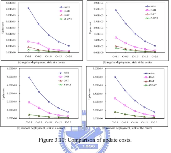
3.10 Comparison of update costs. . . 31
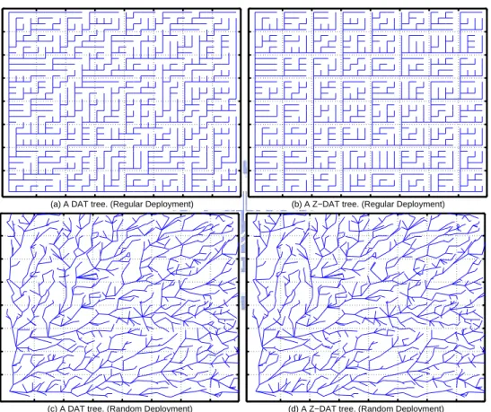
3.11 Snapshots of tree T obtained by DAT and Z-DAT under regular and random deployments. . . 32
3.12 Comparison of update costs under different (α, δ) for Z-DAT. . . . 33
3.13 Comparison of query costs. (C = 1.0) . . . . 34
3.14 Comparison of total costs. (C = 1.0) . . . . 35
4.2 (a) The DLs stored in sensors. (b) An example where Car2
moves from G to I and Car1 moves from H to C. . . . 40
4.3 (a) The query graph G0Car1 of Fig. 4.2(a) for Car1. (b) Another example of a two-tree system. (c) The query graph of (b) for Car1, which contains a cycle. . . 47
4.4 Performance study with objects’ speeds varied, where sensors are deployed regularly and four sinks are deployed. . . 52
4.5 Performance study with objects’ speeds varied, where sensors are deployed regularly and 256 sinks are deployed. . . 54
4.6 Performance study with objects’ speeds varied, where sensors are deployed randomly and four sinks are deployed. . . 55
4.7 Performance study with query rates varied, where sensors are de-ployed regularly and four sinks are dede-ployed. . . 57
4.8 Performance study with query rates varied, where sensors are de-ployed regularly and 256 sinks are dede-ployed. . . 58
4.9 Performance study with the number of sinks varied, where the objects’ speed is set to be 0.333 unit/second. . . 60
4.10 Performance study with the number of sinks varied, where the objects’ speed is set to be 0.111 unit/second. . . 61
4.11 The performance of the partial storage technique. . . 62
5.1 Examples of spatial imprecision and temporal imprecision. . . 66
5.2 A tree-based location management scheme. . . 67
5.3 The values of be queried of sensors collected by (a) ideal-collection and (b) tree-collection, where the DAT tree is used. . . 72
5.4 Some observations. . . 73
5.5 (a) The basic idea of constructing a tree. (b) The problem arising when connecting two subtrees. . . 74
5.6 The impact of objects’ speeds. . . 82
5.7 The impact of query rates. . . 83
5.8 Comparison of ratios of update cost to query cost. . . 83
5.9 The impact of objects’ speeds under two different query scenarios 84 5.10 The impact of query rates under two different query scenarios. . . 84
6.1 Two examples of event reporting in an event-driven WSN. . . 87
6.2 The hidden terminal problem, where Rtran denotes the transmis-sion range of sensors. . . 90
6.3 The redundancy problem. . . 91
6.4 Comparison of slot assignment strategies. . . 96
6.5 The impact of slot size beyond event areas. . . 97
6.6 The advantage of separating flows in time. . . 98
6.7 The synchronization problem. . . 111
6.8 Combining our scheme with LPL. . . 111
6.9 Comparison of different schemes, where Rcorr > Rtran. . . 112
6.10 Comparison of different schemes, where Rcorr < Rtran. . . 113
6.11 The impact of α under different ratios of Rcorr to Rtran. . . 113
6.12 The impact of `, where Rcorr is 15 units, Rtranis 10 units, and the value of α is 0.3. . . . 114
6.13 The impact of `, where Rcorr is 5 units, Rtranis 10 units, and the value of α is 1.0. . . . 114
Chapter 1
Introduction
The emerging wireless sensor network (WSN) technology may greatly facilitate human life. A WSN may consist of many inexpensive wireless nodes, each ca-pable of collecting, processing, and storing environmental information, and com-municating with other nodes. A lot of research efforts have been dedicated to WSNs, including deign of physical and medium access layers [26, 35] and rout-ing and transport protocols [10, 13]. Applications of WSNs have been studied in [2, 6, 17].
Object tracking is an important application of WSNs (e.g., military intrusion detection and habitat monitoring). The key steps involved in tracking include event detection, target classification, and location estimation [3, 5, 15, 18]. In a WSN, when the locations of objects are successfully determined, a location man-agement scheme for reporting objects’ locations and disseminating users’ queries is required [14, 16]. The main theme of this dissertation is location management. In particular, we explore the in-network data processing capability of WSNs by executing distributed location updates and queries inside the network. Updates of an object’s location are initiated when the object moves from one sensor to an-other. A query is invoked each time when there is a need to find the location of an interested object. Location updates and queries may be done in various ways. A naive way for delivering a query is to flood the whole network. The sensor whose sensing range contains the queried object will reply to the query. Clearly,
this approach is inefficient and not scalable because a considerable amount of en-ergy will be consumed when the network scale is large or when the query rate is high. Alternatively, if all location information is stored at a specific sensor (e.g., the sink), no flooding is needed. But whenever a movement is detected, update packets have to be sent to the sink. Thus, when objects move frequently, abundant update packets will be generated. The cost is not justified when the query rate is low. Clearly, these are tradeoffs.
1.1
Location Management for Single-Sink WSNs
In [14], a Drain-And-Balance (DAB) tree structure is proposed to address the issue of location management. As far as we know, this is the first in-network object tracking approach in sensor networks where query messages are not required to be flooded and update messages are not always transmitted to the sink. However, [14] has two drawbacks. First, a DAB tree is a logical tree not reflecting the physical structure of the sensor network; hence, an edge may consist of multiple communication hops and a high communication cost may be incurred. Second, the construction of the DAB tree does not take the query cost into consideration. Therefore, the result may not be efficient in some cases.
In this dissertation, we propose a tree-based location management scheme for single-sink WSNs. We develop several tree structures for in-network object track-ing which take the physical topology of the sensor network into consideration. The optimization process has two stages. The first stage aims at reducing the up-date cost, while the second stage aims at further reducing the query cost. For the first stage, several principles, namely deviation-avoidance and highest-weight-first ones, are pointed out to construct an object tracking tree to reduce the communi-cation cost of locommuni-cation update. Two tree construction algorithms are proposed: Deviation-Avoidance Tree (DAT) and Zone-based Deviation-Avoidance Tree (Z-DAT). The latter approach tries to divide the sensing area into square-like zones, and recursively combine these zones into a tree. Our simulation results indicate
that the Z-DAT approach is very suitable for regularly deployed sensor networks. For the second stage, we develop a Query Cost Reduction (QCR) algorithm to adjust the object tracking tree obtained in the first stage to further reduce the to-tal cost. The way we model this problem allows us to analytically formulate the update and query costs of the solution based on several parameters of the given problem, such as rates that objects cross the boundaries between sensors and rates that sensors are queried. We have also conducted extensive simulations to evaluate the proposed solutions. The results do validate our observations.
1.2
Location Management for Multi-Sink WSNs
We further explore the possibility of having multiple sinks in the network. One advantage of having multiple sinks is to reduce the response time of queries. In addition, using multiple sinks can also relieve the traffic congestion problem as-sociated with a single-sink system (i.e., using multiple sinks can achieve load balance more easily). In order to support location management in a multi-sink sensor network, we can extend the tree structure used in the single-sink system by constructing a logical tree for each sink. However, this implies that updating mul-tiple trees is required when a movement event is detected. Assuming that there are m sinks coexisting in the network, if each tree is updated independently, the update cost will become approximately m times. It is desirable to further reduce the update cost when multiple trees coexist in the network. In this dissertation, by exploring the concept of data aggregation, we propose an algorithm to efficiently update multiple trees. With proper design, we show that the update cost increases slightly when the number of trees (i.e., the number of sinks) increases. Based on the foregoing update algorithm, we formulate the update cost that gives us hints to develop efficient tree-construction algorithms. Two distributed multi-tree con-struction algorithms are presented. Experimental results show that the increased update cost with multiple trees can be compensated by lower query cost and the query cost also depends on m, the number of sinks. This allows us to further
investigate how to choose the value of m under different scenarios.
1.3
Imprecision-tolerant Location Management Model
Since inaccuracy, or even error, of sensing data is inherent for WSNs, applica-tions of WSNs usually have to tolerate some degree of imprecision. This property has been exploited in the design of network protocols for WSNs. For example, precision-constrained data aggregation is considered in [28], and a storage sys-tem that supports drill-down queries with different precision levels is proposed in [11]. Similarly, in moving object environments, maintaining the exact locations of objects anytime is almost infeasible. Not only the positioning results are error-prone, but also the data transfer delay and object mobility make the locations of objects inaccurate. Fortunately, imprecision is tolerable in many object tracking applications. For example, when life scientists intend to track an animal, it may be sufficient to know its moving direction rather than its exact location. In addition, the location information recorded several hours ago, instead of at the current time, may be still available for the life scientists to understand the animal’s daily life.
In this dissertation, we propose an in-network location management scheme to support imprecision-tolerant queries for object tracking sensor networks. We intend to develop a location management model that can achieve two goals. First, multiple imprecision levels should be provided. Second, the query cost should be proportional to the imprecision level. To achieve these two goals, we propose a tree-based imprecision-tolerant location management model. To begin with, we present the update and query mechanisms that can support imprecision-tolerant queries. We then propose a tree construction algorithm to reduce the query cost while minimize the increment of update cost.
1.4
A Link-layer Protocol for Event-driven WSNs
By simulation, we observe that packet loss may make the location information incorrect in object tracking sensor networks. Thus, we also propose a link-layer protocol to relieve the contention and collision problems for event-driven WSNs. We solve these problems by jointly considering two subissues. One is exploiting the spatial correlation of data reported by sensors in the event area, and the other is designing a specific MAC protocol. We propose a novel hybrid TDMA/CSMA protocol with the following interesting features that differentiate itself from con-ventional TDMA-based protocols. First, the TDMA part is based on very loose time synchronization and is triggered by the appearance of events. On the other hand, the CSMA part is adopted in the non-event area to achieve low latency transmission. Second, the slot assignment strategy associated with the TDMA part takes the spatial correlation of sensor data into consideration and thus allows less strict slot allocation than conventional TDMA schemes. Interestingly, by in-tentionally allowing one-hop neighbors to share the same time slot, the number of slots required per frame is significantly reduced. Third, by enlarging the slot size on purpose, our scheme enforces packets, after leaving the event area, to form a pipeline in such a way that packets flow like streams, each of which is separated sufficiently in distance to avoid interference. In addition, by exploiting TDMA’s features and the spatial correlation of sensor data, we show how to reduce redun-dant reports. We also discuss how to combine our protocol with the LPL (Low Power Listening) technique to achieve energy efficiency.
1.5
Organization of This Dissertation
This dissertation is organized as follows. Related works are surveyed in Chap-ter 2. In ChapChap-ter 3, we present the proposed location management scheme for single-sink WSNs. In Chapter 4, we further explore the possibility of having mul-tiple sinks. Based on the tree-based location management schemes, we propose an
imprecision-tolerant location management model in Chapter 5. In Chapter 6, we propose a link layer protocol to solve the packet loss problem that may make loca-tion informaloca-tion incorrect. Finally, we conclude our research results and propose some future directions in Chapter 7.
Chapter 2
Related Works
In this chapter, we first review some papers addressing the object tracking issues in wireless sensor networks. Because the main theme of this dissertation is loca-tion management. In Sec. 2.2, we discuss some existing localoca-tion managements schemes proposed for WSNs. As we mentioned above, packet loss may make location information incorrect. Packet loss is usually caused by contention and collision. We propose a link layer protocol to relieve the contention and collision problems. Because MAC (Medium Access Control) protocols are usually used to solve the contention and collision problems, we review some medium access schemes developed for wireless sensor networks in Sec. 2.3.
2.1
Object Tracking Using Wireless Sensor Networks
A significant amount of research effort has been elaborated upon issues of object tracking problems. The authors in [34] explored a localized prediction approach for power efficient object tracking by putting unnecessary sensors in sleep mode. Techniques for cooperative tracking by multiple sensors have been addressed in [3, 7, 18, 37]. In [7], a dynamic clustering architecture that exploits signal strength observed by sensors is proposed to identify the set of sensors to track an object. In [37], a convoy tree is proposed for object tracking using data aggregation to reduce energy consumption.
2.2
Location Management in Object Tracking
Sen-sor Networks
In [14], a Drain-And-Balance (DAB) tree structure is proposed to address the location management issue. As far as we know, this is the first in-network object tracking approach in sensor networks where query messages are not required to be flooded and update messages are not always transmitted to the sink. However, [14] has two drawbacks. First, a DAB tree is a logical tree not reflecting the physical structure of the sensor network; hence, an edge may consist of multiple communication hops and a high communication cost may be incurred. Second, the construction of the DAB tree does not take the query cost into consideration. Therefore, the result may not be efficient in some cases.
A location management scheme supporting imprecision-tolerant queries for object tracking sensor networks has been studied in [33]. The location information of an object is stored in a centric storage node and a local storage node. When a user intends to know the location of an object, the query will be forwarded from the querying node to the centric storage node of that object. If the precision level is satisfactory, the centric storage node will reply to this query. Otherwise, the query will be forwarded to the local storage node, which has more precise location information of that object. This scheme has two major drawbacks. First, when the querying node is very close to the local storage node of the queried object, the query will still be forwarded to the centric storage node, which may be far from the querying node. Second, only two precision levels are provided.
2.3
MAC Protocols for Wireless Sensor Networks
A significant amount of research effort has been dedicated to the design of MAC protocols for WSNs [1, 20, 22, 24, 27, 29, 30, 35]. The energy efficiency issue has been studied in S-MAC [35] and T-MAC [29] by synchronizing sensors on a com-mon wakeup/sleep schedule. In order to eliminate the synchronization overhead,
B-MAC [20] adopts a preamble sampling technique. Some hybrid TDMA/CSMA MAC protocols have been proposed recently. In Z-MAC [24], some sensors will adopt a CSMA-based MAC protocol and those suffering from high contention will adopt a TDMA-based MAC protocol. By doing so, Z-MAC enjoys the benefits of low latency of CSMA and high channel utilization of TDMA. Funneling-MAC [1] is also a hybrid TDMA/CSMA MAC protocol that aims to solve the funneling ef-fect near the sink. However, these protocols do not address the spatial correlation of sensor data, and thus the contention problem, in event-driven WSNs.
Exploiting the spatial correlation of sensor data on the MAC layer has been discussed in [31], where the relation between the spatial positions of sensors and the event estimation reliability is investigated. Specifically, a distortion function is derived and a term correlation radius (Rcorr) is introduced. Then, CC-MAC
(spatial Correlation-based Collaborative Medium Access Control) is proposed. CC-MAC consists of two components: E-MAC (Event MAC) and N-MAC (Net-work MAC). E-MAC aims to filter out correlated reporting (i.e., determine which sensors can report). On the other hand, N-MAC is mainly used for sensors not in the event area to forward reporting packets. However, CC-MAC has the fol-lowing drawbacks: (i) E-MAC is a pure contention-based protocol. Although some sensors may withdraw from reporting, those sensors that decide to report will still cause a lot of contention, because they will report simultaneously. (ii) The RTS/CTS mechanism is adopted, which causes high overheads when packet sizes are small. (iii) In CC-MAC, when a sensor x overhears a packet reported by another sensor y, x will judge whether the distance between itself and y is smaller than Rcorr. If so, x will suspend its report. As to be shown later, this simple
condition cannot completely avoid redundant reporting. (iv) The report reduction technique proposed in CC-MAC highly depends on overhearing; thus, redundancy may still exist when when one misses overhearing.
Chapter 3
In-network Location Management
for the Single-sink System
In this chapter, we present our proposed location management scheme designed for the single-sink sensor networks. We propose a tree structure for in-network object tracking in a sensor network. The location update part of our solution can be viewed as an extension of [14]. In particular, we take the physical topology of the sensor network into consideration. We take a two-stage approach. The first stage aims at reducing the update cost, while the second stage aims at further reducing the query cost. For the first stage, several principles, namely deviation-avoidance and highest-weight-first ones, are pointed out to construct an object tracking tree to reduce the communication cost of location update. Two solutions are proposed: Deviation-Avoidance Tree (DAT) and Zone-based Deviation-Avoidance Tree (Z-DAT). The latter approach tries to divide the sensing area into square-like zones, and recursively combine these zones into a tree. Our simulation results indicate that the Z-DAT approach is very suitable for regularly deployed sensor networks. For the second stage, we develop a Query Cost Reduction (QCR) algorithm to adjust the object tracking tree obtained in the first stage to further reduce the total cost. The way we model this problem allows us to analytically formulate the update and query costs of the solution based on several parameters of the given problem, such as rates that objects cross the boundaries between sensors and rates that sensors are queried. We have also conducted extensive simulations to evaluate
36 17 16 23 8 15 A B 12 6 C 23 12 D 7 3 9 3 E 5 11 17 6 F 21 12 2 5 G H I J K 12 8 1 0 2 5 11 9 8 6 9 6 10 9 13 25 5 8 13 15 9 12 (a) A B C D E F G H I J K 33 18 10 35 23 12 16 15 7 39 23 20 14 20 53 19 38 13 28 7 1 21 (b)
Figure 3.1: (a) The Voronoi graph of a sensor network. (b) The graph G corre-sponding to the sensor network in (a).
the proposed solutions. The results do validate our observations.
3.1
Preliminaries
We consider a wireless sensor network deployed in a field for the purpose of object tracking. Sensors’ locations are already known at a special node, called sink, which serves as the gateway of the sensor network to the outside world. We adopt a simple nearest-sensor model, which only requires the sensor that receives the strongest signal from the object to report to the sink (this can be achieved by [7]). Therefore, the sensing field can be partitioned into a Voronoi graph [4], as depicted in Fig. 3.1(a), such that every point in a polygon is closer to its corresponding sensor in that polygon than to any other. In practice, a sensor under our model may represent the clusterhead of a cluster of reduced-function sensors. In this work, however, we are only interested in the reporting behavior of these clusterheads.
Our goal is to propose a data aggregation model for object tracking. We as-sume that whenever an object arrives at or departs from the sensing range (poly-gon) of a sensor, a detection event will be reported (note that this update message
are not always forwarded to the sink, as will be elaborated later). Two sensors are called neighbors if their sensing ranges share a common boundary on the Voronoi graph; otherwise, they are non-neighbors. Multiple objects may be tracked con-currently in the network, and we assume that from mobility statistics, it is possi-ble to collect the event rate between each pair of neighboring sensors to represent the frequency of objects travelling from one sensor to another. For example, in Fig. 3.1(a), the arrival and departure rates between sensors are shown on the edges of the Vonoroi graph. Note that before the statistics is done, the initial weights can be the same value for all edges. In addition, the communication range of sensors is assumed to be large enough so that neighboring sensors (in terms of their sensing ranges) can communicate with each other directly. Thus, the network topology can be regarded as an undirected weighted graph G = (VG, EG) with VG
rep-resenting sensors and EG representing links between neighboring sensors. The
weight of each link (a, b) ∈ EG, denoted by wG(a, b), is the sum of event rates
from a to b and b to a. This is because both arrival and departure events will be reported in our scheme. In fact, G is a Delaunay triangulation of the network [4]. Fig. 3.1(b) shows the corresponding Delaunay triangulation of the sensor network in Fig. 3.1(a). Note that the number labelled on each edge represents its weight.
In light of the storage in sensors, the sensor network is able to be viewed as a distributed database. We will exploit the possibility of conducting in-network data aggregation for object tracking in a sensor network. Similar to the approach in [14], a logical weighted tree T will be constructed from G. Note that T may not be a spanning tree in which each node’s parent is its neighbor. For example, Fig. 3.2(a) shows an object tracking tree T constructed from the network G in Fig. 3.1(b), where the dotted lines are the forwarding path of a query for Car1. Movement events of objects are reported based on the following rules. Each node
a in T will maintain a detected list DLa = (L0, L1, . . . , Lk) such that L0 is the set
of objects currently inside the coverage of sensor a itself, and Li, i = 1, · · · , k,
is the set of objects currently inside the coverage of any sensor who is in the subtree rooted at the i-th child of sensor a, where k is the number of children of a.
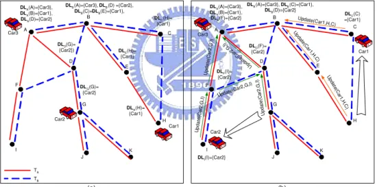
A B C D E F G H I J K Q u er y (C a r1 ) Car1 Car2 Car3
DLA({Car3}, {Car1}, NIL,NIL , {Car2})
DLB(NIL, {Car2}, NIL, NIL )
DLF(NIL, {Car1}) w T(I,J) = 1 w T (F ,I ) = 1 w T(J,K) = 1 w T (A ,F ) = 1 DLD(NIL) w T(A ,G ) = 2 w T(A ,D ) = 1 DLC(NIL ) w T(B,C) = 1 wT(A,B) = 1 w T(B ,E ) = 1 w T(B ,H ) = 2 DLG(NIL) DLE(NIL) DLH({Car2} ) DLK({Car1} ) DLJ(NIL, {Car1} )
DLI(NIL, {Car1} )
Q u e ry (C a r1 ) Query(Car1) Query(Car1) A is the sink. (a) A B C D E F G H I J K (b) A is the sink. Car1 Car2 Car3
DLA({Car3}, NIL, {Car1}, NIL, {Car2})
DLB(NIL, NIL, NIL, {Car2})
DLC({Car2}) DLE(NIL) DLF(NIL, NIL) DLG({Car1}) dep( C ar2, H , C) arv(Car2, C, H) arv (C ar1 , G , K ) Q ue ry (C ar1 ) DLH(NIL) DLK(NIL) dep(Car1, K, G) DLJ(NIL, NIL) DLI(NIL, NIL) d ep (C a r1 , K , G ) dep(Car1, K, G) d e p (C ar 1 , K , G ) DLD(NIL)
Figure 3.2: (a) An object tracking tree T . (b) The events generated as Car1 moves from sensor K to G and Car2 moves from H to C.
When an object o moves from the sensing range of a to that of b ((a, b) ∈ EG), a
departure event dep(o, a, b) and an arrival event arv(o, b, a) will be reported by a and b, respectively, alone the tree T . On receiving such an event, a sensor x takes the following actions:
• If the event is dep(o, a, b), x will remove o from the proper Li in DLxsuch
that sensor a belongs to the i-th subtree of x in T . If x = a, o will be removed from L0 in DLx. Then x checks whether sensor b belongs to the
subtree rooted at x in T or not. If not, the event dep(o, a, b) is forwarded to the parent node of x in T .
• If the event is arv(o, b, a), x will add o to the proper Li in DLx such that
sensor b belongs to the i-th subtree of x in T . If x = b, o will be added to
L0in DLx. Then x checks whether sensor a belongs to the subtree rooted at
x in T or not. If not, the event arv(o, b, a) is forwarded to the parent node
of x in T .
The above data aggregation model guarantees that, disregarding transmission delays, the data structure DLialways maintains the objects under the coverage of
Table 3.1: Summary of notations used in Chapter 3.
distG(u, v) The minimum hop count between u and v in G.
distT(u, v) The sum of wTs of edges on the path connecting u and v in T .
wG(u, v) The event rate between u and v.
wT(u, v) The weight of edge (u, v) in T . (= distG(u, v)).
lca(u, v) The lowest common ancestor of u and v.
p(v) The parent of v in T .
Subtree(v) Members of the subtree rooted at v.
root(v) The root of the temporary subtree containing v during the construction of T .
q(v) The query rate of v.
neighbors(v) Neighbors of v. children(v) Children of v.
any descendant of sensor i in T . Therefore, searching the location of an object can be done efficiently in T ; a query is only required to be forwarded to a proper subtree and no flooding is needed. For example, Fig. 3.2(a) shows the forwarding path of a query for Car1 in T . Fig. 3.2(b) shows the reporting events as Car1 and Car2 move and the forwarding path of a query for the new location of Car1.
Our goal is to construct an object tracking tree T = (VT, ET) that incurs
the lowest communication cost given a sensor network G = (VG, EG) and the
corresponding event rates and query rates, where VT = VG and ET consists of
|VT| − 1 edges with the sink as the root. Intuitively, T is a logical tree constructed
from G, in which each edge (u, v) ∈ T is one of the shortest paths connecting sensors u and v in G. Therefore, the weight of each edge (u, v) in T , denoted by
wT(u, v), is modelled by the minimum hop count between u and v in G. The cost
function can be formulated as C(T ) = U (T ) + Q(T ), where U (T ) denotes the update cost and Q(T ) is the query cost.
3.2
Tree Construction Algorithms
This section presents our algorithms to construct efficient object tracking trees. In Section 3.2.1, we develop algorithm DAT targeted at reducing the update cost. Then, in Section 3.2.2, based on the concept of divide-and-conquer, we devise algorithm Z-DAT to further reduce the update cost. In Section 3.2.3, algorithm QCR is developed to adjust the tree obtained by algorithm DAT/Z-DAT to further reduce the total cost.
3.2.1
Algorithm DAT (Deviation-Avoidance Tree)
Object tracking typically involves two basic operations: update and query. Based on the aggregation model in Section 3.1, updates will be initiated when an object
o moves from sensor a to sensor b. It can be seen that both the departure event dep(o, a, b) and the arrival event arv(o, b, a) will be forwarded to the root of the
minimum subtree containing both a and b. Therefore, the update cost U (T ) of a tree T can be formulated by counting the average number of messages transmitted in the network per unit time:
U(T ) = X
(u,v)∈EG
wG(u, v) × (distT(u, lca(u, v)) + distT(v, lca(u, v))), (3.1)
where lca(u, v) denotes the root of the minimum subtree in T that includes both u and v (from now on, we will call lca(u, v) the lowest common ancestor of u and
v), and distT(x, y) is the sum of weights of the edges on the path connecting x
and y in T . For example in Fig. 3.2(a), distT(F, K) = wT(F, I) + wT(I, J) +
wT(J, K) = 3. In order to identify which factors affecting the value of U(T ), we
show that U (T ) also can be formulated in a different way as follows.
Theorem 1. Given any logical tree T of the sensor network G, we have
U(T ) = X (p(v),v)∈ET wT(p(v), v) × X (x,y)∈EG∧x∈Subtree(v) ∧y /∈Subtree(v) wG(x, y) , (3.2)
where Subtree(v) is the subtree of T rooted at node v and p(v) is the parent of v.
Proof. This can be proved by observing which events will be reported along an edge in T . Given (p(v), v) ∈ ET, for any (x, y) ∈ EG where x ∈ Subtree(v)
and y /∈ Subtree(v), since the lowest common ancestor of x and y must not in Subtree(v), any event generated on (x, y) will be transmitted from v to p(v). Otherwise, no message will be transmitted from v to p(v). This leads to the theo-rem.
From Eq. 3.1 and Eq. 3.2, we make three observations about U (T ):
• Eq. 3.1 contains the factor distT(u, lca(u, v)). Its minimal value is
distG(u, lca(u, v)), which denotes the minimum hop count between sensor
u and sensor lca(u, v) in G. Therefore, we would expect that distT(u, sink) = distG(u, sink) for each u ∈ VG; otherwise, we say that u deviates from
its shortest path to the sink. If distT(u, sink) = distG(u, sink) for each
u ∈ VG, we say that tree T is a deviation-avoidance tree. Fig. 3.3 shows
four possible object tracking trees for the graph G in Fig. 3.1(b). The one in Fig. 3.3(b) is not a deviation-avoidance tree since distT(E, A) = 3 >
distG(E, A) = 2. The other three are deviation-avoidance trees.
• Eq. 3.2 contains the factor wT(u, v). Its minimal value is 1 when u 6= v.
Consequently, it is desirable that each sensor’s parent is one of its neigh-bors. Only the tree in Fig. 3.3(d) satisfies this criterion. By selecting neighboring sensors as parents, the average value of distT(u, lca(u, v)) +
distT(v, lca(u, v)) in Eq. 3.1 can be minimized. For example, the
aver-age values of distT(u, lca(u, v)) + distT(v, lca(u, v)) are 3.591, 2.864, and
2.227 for the trees in Fig. 3.3(a), 3.3(c), and 3.3(d), respectively.
• In Eq. 3.1, the weight wG(u, v) will be multiplied by distT(u, lca(u, v)) +
A B C D E F G H I J K (a) A is the sink. w T(A,B) = 1 w T(A,C) = 2 w T(A,E ) = 2 w T(A ,H ) = 3 w T(A ,D ) = 1 w T(A ,K ) = 3 w T(A ,G ) = 2 w T(A ,J ) = 3 w(AT ,F) = 1 wT (A ,I) = 2 A B C D E F G H I J K A is the sink. wT(A,B) = 1 w T(A,C) = 2 wT(C ,E) = 1 w T(D ,H) = 2 w T(A ,D ) = 1 w T(F,K ) = 2 w T (D ,G ) = 1 w T(F ,J) = 2 w T (A ,F ) = 1 w T (F ,I ) = 1 (b) A B C D E F G H I J K A is the sink. wT(A,B) = 1 w T(A,C) = 2 w T(D,E) = 1 w T(D ,H ) = 2 w T(A ,D ) = 1 w T(F,K ) = 2 w T (D ,G ) = 1 w T(F ,J) = 2 w T (A ,F ) = 1 w T (F ,I ) = 1 (c) A B C D E F G H I J K A is the sink. wT(A,B) = 1 w T(B,C) = 1 w T(D,E) = 1 w T(E ,H ) = 1 w T(A ,D ) = 1 w T(G ,K ) = 1 w T (D ,G ) = 1 w T (G ,J ) = 1 w T (A ,F ) = 1 w T (F ,I) = 1 (d)
Figure 3.3: Four possible location tracking trees for the graph in Fig. 3.1(b).
> wG(u0, v0), it is desirable that distT(u, lca(u, v)) + distT(v, lca(u, v)) <
distT(u0, lca(u0, v0)) + distT(v0, lca(u0, v0)). Combining this observation
with the second observation, an edge (u, v) with a higher wG(u, v) should
be included into T as early as possible and p(v) should be set to u if
distG(u, sink) < distG(v, sink), and vice versa. We call this the
highest-weight-first principle.
Based on above observations, we develop our algorithm DAT. Initially, DAT treats each node as a singleton subtree. Then we will gradually include more links to connect these subtrees together. In the end, all subtrees will be connected into one tree T . The detailed algorithm is shown in Algorithm 1, where notation
root(x) represents the root of the temporary subtree that contains x. To begin
on the third observation, algorithm DAT will examine edges in L one by one for possibly being included into tree T . For each edge (u, v) in L being examined by algorithm DAT, (u, v) will be included into T only if u and v are currently located in different subtrees. Also, (u, v) will be included into T only if at least one of u and v is currently the root of its temporary subtree and the other is on a shortest path in G from the former node to the sink (these conditions are reflected by the
if statements in lines 5 and 7). An edge in G passing these checks will then be
included into T . Note that without these conditions, deviations may occur. It can be seen that T is always a subgraph of G and wT(u, v) = 1 for all (u, v) ∈ ET.
For example, Fig. 3.4(a) is a snapshot of an execution of DAT. The solid lines are those edges that have been included into T . When (F, G) is examined by DAT, it will not be included into T , because neither F nor G is the root of its temporary subtree. Another snapshot is shown in Fig. 3.4(b). When (B, D) is examined, it will not be included into T . Although D is the root of its temporary subtree, B is not on the shortest path from D to A, i.e., distG(D, A) 6= distG(B, A)+1. (A, D)
will be then examined after (B, D). (A, D) can be included into T , because D is the root of its temporary subtree and A is on the shortest path from D to A.
Algorithm 1 DAT(G)
1: Let T = (VT, ET) such that VT = VGand ET = φ
2: Sort EGinto a list L in a decreasing order of their event rates.
3: for each (u, v) ∈ EGin L do
4: if (root(u) 6= root(v)) then
5: if (u = root(u)) ∧ (distG(u, sink) = distG(v, sink) + 1) then
6: Let ET = ET ∪ (u, v) and let the root of the new subtree be root(v).
7: else if (v = root(v)) ∧ (distG(v, sink) = distG(u, sink) + 1) then
8: Let ET = ET ∪ (u, v) and let the root of the new subtree be root(u).
9: end if
10: end if
11: end for
Theorem 2. If G is connected, the tree T constructed by algorithm DAT is a
A B C D E F G H I J K 33 18 10 35 23 12 16 15 7 39 23 20 14 20 53 19 38 13 28 7 1 21 (a) Root node Non-root node (Sink) A B C D E F G H I J K 33 18 10 35 23 12 16 15 7 39 23 20 14 20 53 19 38 13 28 7 1 21 (b) (Sink) Root node Non-root node
Figure 3.4: Snapshots of an execution of DAT.
Proof. First, we show that T is connected. Each sensor is the root of a singleton subtree in the beginning and we will prove that only one senor will be the root in the ending. Since G is connected, when a sensor x 6= sink is the root of a subtree (i.e., x = root(x)), it always can find a neighboring sensor y such that distG(x, sink) = distG(y, sink) + 1. It is clear that root(y) 6= x, because
distG(root(y), sink) ≤ distG(y, sink). Hence, edge (x, y) can be included into
T , and x will not be the root anymore. By repeating such arguments, T must be
connected and rooted at the sink. Second, we show that T is a deviation-avoidance tree. This can be derived from two observations. First, when an edge (u, v) is included into T , DAT will choose v as the child of u if distG(v, sink) is larger
than distG(u, sink), and vice versa. Therefore, if the path from the sink to sensor
u is one of the shortest paths, the path from the sink to sensor v is also one of the
shortest paths. Second, assuming distG(v, sink) = distG(u, sink) + 1, DAT will
include (v, u) only when v itself is the root of a subtree. This guarantees that all descendant nodes in Subtree(v) will not deviate from their shortest paths to the sink. Hence, the theorem follows.
3.2.2
Algorithm Z-DAT (Zone-based Deviation-Avoidance Tree)
The Z-DAT is derived based on the following locality concept. Assume that u is v’s parent in T . According to Eq. 3.2, for any edge (x, y) ∈ EG such that
x ∈ Subtree(v) and y /∈ Subtree(v), arrival/departure events between x and y
will cause a message to be transmitted on (p(v), v), thus increasing the value of
P
(x,y)∈EG∧x∈Subtree(v)∧y /∈Subtree(v)wG(x, y). Therefore, the perimeter that bounds
the sensing area of sensors in each Subtree(v) will impact the update cost U (T ). A longer perimeter would imply more events crossing the boundary. For example, in the three subtrees in Fig. 3.5, although all subtrees have the same number of sensors, the perimeter of the subtree in Fig. 3.5(a) is smaller than that in 3.5(b), which is in turn less than that in 3.5(c). In geometry, it is clear that a circle has the shortest perimeter to cover the same area as compared with other shapes. Circle-like shapes, however, are difficult to be used in an iterative tree construction. As a result, Z-DAT will be developed based on square-like zones.
(a) (b) v v (c) v p(v) p(v) p(v)
Figure 3.5: Possible structures of subtrees with nine sensors.
Z-DAT is derived based on the deviation-avoidance principle and the above locality concept. The algorithm builds T in an iterative manner based on two parameters, α and δ, where α is a power of 2 and δ is a positive integer. To begin with, Z-DAT first uses (α − 1) horizontal lines to divide the sensing field into α strips. For each horizontal line between two strips, we are allowed to further move it up and down within a distance no more than δ units. This gives 2δ + 1 possible locations of each horizontal line. For each location of the horizontal line, we can
calculate the total event rate that objects may move across the line. Then we pick the line with the lowest total event rate as its final location. After all horizontal lines are determined, we then further partition the sensing field into α2regions by using (α − 1) vertical lines. Following the adjustment as above, each vertical line is also allowed to move left and right within a distance no more than δ units and the one with the lowest total event rate is selected as its final location.
After the above steps are completed, the sensing field is divided into α2 square-like zones. First, we run DAT on the sensors in each zone. This will result in one or multiple subtrees in each zone. Next, we will merge subtrees in the above α2 zones recursively as follows. First, we combine these zones together into α2 × α2 larger zones, such that each larger zone contains 2 × 2 neighboring zones. Then we merge subtrees in these 2 × 2 zones by sorting all inter-zone edges (i.e., edges connecting these 2×2 zones) according to their event rates into a list L and feeding
L to steps 3 ∼ 11 of the original DAT algorithm. Second, we further combine the
above larger zones together into α4 × α4 even larger zones, such that each even larger zone contains 2 × 2 neighboring larger zones. This process is repeated until one single tree is obtained. The algorithm is summarized in Algorithm 2. An illustrated example is shown in Fig. 3.6. In the first iteration, we divide the field into α×α zones and adjust their boundaries according to δ as shown in Fig. 3.6(a). In the second iteration, each 2 × 2 neighboring zones is combined into a larger zone as shown in Fig. 3.6(b).
Algorithm 2 Z-DAT(G, α, δ)
1: Divide the network into α × α zones based on parameters α and δ.
2: Run DAT on the sensors in each zone.
3: i ← 1
4: while 2αi 6= 0 do
5: The network is divided into 2αi ×2αi zones.
6: Run DAT on each zone to merge its subtrees.
7: i ← i + 1
8: end while
Zone12 Zone11 Zone10 Zone9 Zone8 Zone5 Zone6 Zone2 Zone1 Zone15 Zone14 Zone7 Zone3 Zone4 Zone13 Zone16 (a) 2 Zone2 Zone4 Zone3 Zone1 (b)
Figure 3.6: An example of the Z-DAT algorithm with α = 4.
in a different order. By partitioning the sensing field into zones, each subtree in
T is likely to cover a square-like region, thus avoiding the problem pointed out
in Fig. 3.5. Also, by using the parameter δ to fine-tune the lowest-level zones, Z-DAT tends to avoid high-weight links becoming inter-zone edges. In fact, this is a consequence of the the highest-weight-first design principle.
Theorem 3. If G is connected, the tree T constructed by algorithm Z-DAT is a
connected deviation-avoidance tree rooted at the sink.
Proof. Z-DAT will examine all links of G, but in a different order from DAT. However, the proof of Theorem 5 is independent of the order of the links being examined for being included into T . Therefore, the same proof is still applicable here.
3.2.3
Algorithm QCR (Query Cost Reduction)
The above DAT and Z-DAT only try to reduce the update cost. The query cost is not taken into account. QCR is designed to reduce the total update and query cost by adjusting the object tracking tree obtained by DAT/Z-DAT. To begin with, we define the query rate q(v) of each sensor v as the average number of queries that refer to objects within the sensing range of v per unit time in statistics.
Given a tree T , we first derive its query cost Q(T ). Suppose that an object x is within the sensing range of v. When x is queried, if v is a non-leaf node, the query message is required to be forwarded to v since p(v) only indicates that x is in the subtree rooted at v. On the other hand, if v is a leaf node, the query message only has to be forwarded to p(v), because sensor p(v) knows that the object is currently monitored by v. The following equation gives Q(T ) by taking into account the number of hops that query requests and query replies have to travel on T .
Q(T ) = 2 × X v∈VT ∧ v /∈leaf node q(v) × distT(v, sink) + X v∈VT ∧ v∈leaf node q(v) × distT(p(v), sink) ,(3.3)
We make two observations on Q(T ). First, because distT(p(v), sink) is
al-ways smaller than distT(v, sink), Eq. 3.3 indicates that placing a node as a leaf
can save the query cost instead of placing it as a non-leaf. For example, when query rates are extremely high, it is desirable that every node will become a leaf node and T will become a star-like graph. Second, the second term in Eq. 3.3 implies that the value of distT(p(v), sink) should be made as small as possible.
Thus, we should choose a node closer to the sink as v’s parent (however, this is at the expense of the update cost).
Based on the above observations, QCR tries to adjust the tree T obtained by DAT or Z-DAT. In QCR, we examine T in a bottom-up manner and try to adjust the location of each node in T by the following operations.
1. If a node v is not a leaf node, we can make it a leaf by cutting the links to its children and connecting each of its children to p(v). (Note that we can do so because T is regarded as a logical tree.) Let T0 be the new tree after
modification. We derive that C(T ) − C(T0) = Q(T ) − Q(T0) + U(T ) − U(T0) = 2 × q(v) + X i∈children(v)∧ i∈leaf node q(i) − X i∈neighbors(v) ∧i∈Subtree(v) wG(v, i) − X i∈children(v) X (x,y)∈EG∧y /∈Subtree(i) ∧x∈Subtree(i) wG(x, y) + X (x,y)∈EG∧y /∈Subtree(v) ∧x∈Subtree(v)∧x6=v wG(x, y). (3.4)
If the amount of reduction is positive, we replace T by T0. Otherwise, we keep T unchanged. Fig. 3.7 illustrates this operation.
w
v
u
1u
kw
v
u
1u
ku
2u
2Figure 3.7: Making a non-leaf node v a leaf node.
2. If a node v is a leaf node, we can make p(v) closer to the sink by cutting v’s link to its current parent p(v) and connect v to its grandparent p(p(v)). Let
T0 be the new tree. We derive that
C(T ) − C(T0) = Q(T ) − Q(T0) + U(T ) − U(T0) = 2 × (q(v) + q0(v)) − 2 × X (x,y)∈EG∧y /∈Subtree(v)∧ x∈Subtree(v)∧y∈Subtree(p(v)) wG(x, y) , (3.5)
where
q0(v) = ½
0 if p(v) has more than one child in T
q(p(v)) otherwise .
If the amount of reduction is positive, we replace T by T0. Otherwise, T remains unchanged. Fig. 3.8 illustrates this operation.
w
u
v
1v
iv
kw
u
v
1v
iv
kFigure 3.8: Connecting a leaf node vito p(p(vi)).
Note that Eq. 3.4 and Eq. 3.5 allow us to compute the reduction of cost without computing U (T0) and Q(T0). This saves computational overhead. Also note that
T is examined in a bottom-up manner in a layer-by-layer manner. Nodes that are
moved to an upper layer will have a chance to be reexamined. However, to avoid going back and forth, nodes that are not moved will not be reexamined.
For example, suppose that we are given a DAT tree in Fig. 3.9(a) (which is constructed from Fig. 3.1(b)), where the number labelled on each node is its query rate. When examining the bottom layer, we will apply step 2 to sensors H, J , and
K and obtain reductions of 1974, −62, and −6, respectively. Hence, only H is
moved upward as shown in Fig. 3.9(b). When examining the second layer, we will apply step 1 to sensor G and I and apply step 2 to sensors C, E, and H. Only when applying to sensor H, it will result in a positive reduction of 1970. This updates the tree to Fig. 3.9(c). Finally, sensors B, D, and F are examined. Only
D has a positive reduction of 1842. Thus, D will become a leaf and all its children
are connected to D’s parent as shown in Fig. 3.9(d). Overall, the cost is reduced from 7124 to 5150, 3180, and then 1338 after each step respectively.