人眼視覺導向之低功耗液晶顯示器背光管理

(1)

國立交通大學

電機學院光電顯示科技產業研發碩士班

碩士論文

人眼視覺導向之低功耗液晶顯示器背光管理

Visual Perception-Guided Low-Power LCD

Backlight Management

研究生：趙健富

指導教授：鄭惟中博士

(2)

人眼視覺導向之低功耗液晶顯示器背光管理

Visual Perception-Guided Low-Power LCD

Backlight Management

研究生: 趙健富

Student: Chien-Fu Chao

指導教授: 鄭惟中博士 Advisor: Dr. Wei-Chung Cheng

國立交通大學

電機學院光電顯示科技產業研發碩士班

碩士論文

A Thesis

Submitted to College of Electrical and Computer Engineering

National Chiao Tung University

in Partial Fulfillment of the Requirements

for the Degree of

Master

in

Industrial Technology R & D Master Program on

Photonics and Display Technologies

February 2007

Hsinchu, Taiwan, Republic of China

(3)

人眼視覺導向之低功耗液晶顯示器背光管理

碩士研究生：趙健富指導教授：鄭惟中博士

國立交通大學電機學院

中文摘要

以人眼視覺感受為導向，我們提供了一個三色背光調節(backlight scaling)的演算法，藉著影像的統計圖，分別調節該影像紅、藍、綠三色的背光強度。該演算法分成二部分，第一部分為色度調節，在一個給定的色差條件下找出紅、藍、綠三色光的比率。第二部分為亮度調節，在可察覺的明度差異下調節背光模組的亮度，同時，我們利用心理物理實驗去找到最佳的亮度轉移函數。為了實現該演算法，我們並架設一組實驗平台來量測實行演算法之後的效果。在所有選定的測試影像(benchmark image)中，我們量測出最多可以節省55%的LED背光模組功率消秏，且兼顧該顯示影像的品質。

(4)

Visual Perception-Guided Low-Power LCD

Backlight Management

Student：Chien-Fu Chao Advisor：Dr. Wei-Chung Cheng

National Chiao Tung University

ABSTRACT

This study presents an algorithm for minimizing power consumption of LED backlights in transmissive TFT-LCD monitors. The proposed algorithm reduces power consumption by scaling the luminous intensity of the red, green, and blue LED backlights independently according to the image histograms of each color channel. The algorithm consists of two phases. The first phase, chromaticity scaling, finds the optimal ratios of red, green, and blue backlights subject to a perceived color difference constraint. The second phase, luminance scaling, finds the optimal dimming factor subject to a perceived lightness difference constraint. The perceived color and lightness differences are measured by the CIELAB Color Difference Equation 2 ∆Eab* , a standard metric for measuring color variation. Psychophysical experiments were performed to uncover the optimal luminance scaling function. The Chromaticity-Luminance Scaling algorithm was implemented in a prototype. Within limited perceivable difference 2∆Eab* , up to 55% of power consumption can be reduced for the benchmark images.

(5)

致謝

回憶這兩年的日子，有歡欣的微笑也有辛勤的汗水。一路上，受到眾人的扶持與關懷，讓我能夠順利完美地劃下句點。在此，謹以該論文表達對你們誠摯的謝意。兩年的研究生活與論文的完成，首先要感謝鄭惟中老師，您不只提供優良的學習環境，也給予我學習機會，並且花費不少精神和時間指導我，不僅讓我在專業工具、語言、做事方法各方面都具有相當顯著的提升，更重要的是讓我有更具彈性的思維以及正向的思考，並用不同層面的觀點來看待事物及問題，在此誠心的謝謝您！在這段求學的日子裡，感謝所有研究所的好夥伴枝福、淑萍、建智、俊文、俞文、映頻、愷均、浩瑜、佳峰、明倫等，在課業上、研究上、生活上的幫助與分享，因為有你們，我的研究生活變得十分有趣，另可能尚有未提及但是曾經幫助過我的朋友們，在此均一併致謝。你們的陪伴讓我在兩年的研究生活過的快樂又充實。在此，特別要感謝枝福和淑萍，不論是我在研究過程或是生活方面遇到挫折或困難，你們都不吝於給我幫助和建議，充分予我堅持到底的力量，讓我順利完成我的學位，謝謝你們！最後感謝我的家人們，是你們在我背後默默的支持，讓我毫無後顧之憂，專注在自己的學習崗位上。因為你們的付出與鼓勵，堅定我辭去工作重拾書本的信念，最後我才可以順利完成我的研究，沒有你們的付出和支持，我相信今天的我不會有如此的成就，在這裡表達我最由衷的感謝，也將這篇論文獻給我最摯愛的家人們。

(6)

List of Tables

Table 6-1. The FPGA chip usage... 55 Table 7-1. Benchmark images. ... 61 Table 7-2. Optimal solutions for benchmark images subject to ∆Eab* ≤1 and

2 * ≤

(9)

List of Figures

Figure 1-1. TFT-LCD Architecture. ... 3

Figure 1-2. LCD subsystem architecture... 3

Figure 1-3. PC system and LCD component architecture. ... 4

Figure 1-4. Power, backlight, transmittance, and luminance. ... 4

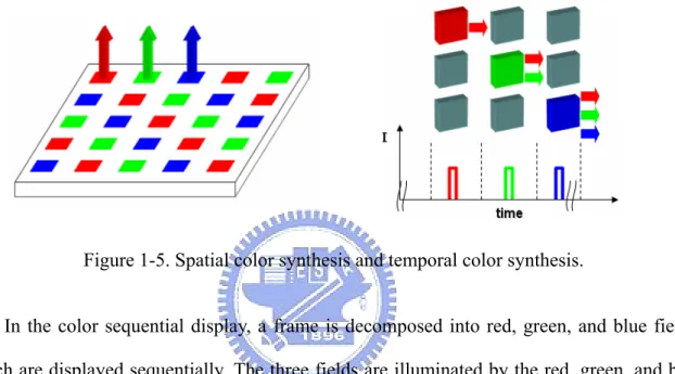
Figure 1-5. Spatial color synthesis and temporal color synthesis... 6

Figure 1-6. The red, green, and blue field of a frame... 6

Figure 2-1. Night Watch (a) Rembrandt (b) Choi (c) Iranli (d) Cheng... 9

Figure 3-1. Illustration of LED backlight and photometric terms. ... 12

Figure 3-2. The CIE color matching functions for the 1931 Standard Colorimetric Observer... 14

Figure 3-3. The CIE x,y chromaticity diagram. ... 15

Figure 3-4. CIE-Lab chromaticity diagram. ... 16

Figure 3-5. Results of determining the brightness functions under different states of adaptation [24]... 19

Figure 3-6. Change in lightness contrast as function of adapting luminance according to the Stevens effect [25]. ... 20

Figure 3-7. Changes in lightness contrast as a function of surround relative luminance according to the results of Bartleson and Breneman [22][29]... 20

Figure 4-1. The experimental apparatus. ... 23

Figure 4-2. The sinusoidal grating pattern with varied apparent brightness and contrast. ... 23

Figure 4-3. Contrast versus related luminance. ... 25

Figure 4-4. The setup of darkroom. ... 26

Figure 4-5. The LED lights... 26

Figure 4-6. TFT-LCD monitors used in the experiments. ... 27

Figure 4-7. GretagMacBeth Eye-One XT... 27

Figure 4-8. Matching the original softcopy (left) with the contrast-adjusted one (right). ... 28

Figure 4-9. The image contrast was modulated between high (left) and low (right). ... 28

Figure 4-10. Subject count vs. contrast adjustment for ascending (bottom) and descending (top) trials. ... 29

Figure 4-11. Contrast fidelity vs. contrast. ... 30

Figure 5-1. Photo and R, G, and B histogram... 31

(10)

Figure 5-3. Transfer functions of chromaticity and luminance scaling... 34

Figure 6-1. Backlight scaling of portable electronic device... 35

Figure 6-2. Our notion of backlight scaling. ... 36

Figure 6-3. Block diagram of image processing flow. ... 37

Figure 6-4. Fetching the image data as the image data is delivered by graphic card. ... 38

Figure 6-5. Fetching the image data as the image data passes the scaler board... 38

Figure 6-6. Simplified diagram of LVDS driver and receiver. ... 39

Figure 6-7. VX912 monitor and panel... 40

Figure 6-8. Block diagram of the AUO panel. ... 41

Figure 6-9. Xilinx Spartan-3 Starter Kit Board [31]. ... 42

Figure 6-10. LED and LED backlight. ... 43

Figure 6-11. Block diagram of backlight module... 43

Figure 6-12. LED backlight driving board. ... 43

Figure 6-13. Chroma meter... 44

Figure 6-14. Power supply... 44

Figure 6-15. Multimeter... 44

Figure 6-16. Layout of experimental system... 45

Figure 6-17. Waveform chart of video signal (a). ... 47

Figure 6-18. Waveform chart of video signal (b). ... 47

Figure 6-19. Waveform chart of video signal (c). ... 48

Figure 6-20. TTL data inputs mapped to LVDS outputs [32]... 49

Figure 6-21. Basic hierarchy of the HDL code... 50

Figure 6-22. The histogram calculation module... 50

Figure 6-23. The boundary determination block. ... 51

Figure 6-24. The circuit scheme of backlight adjusting hierarchy. ... 52

Figure 6-25. The PWM Generator. ... 52

Figure 6-26. The circuit scheme of transmittance adjusting hierarchy... 53

Figure 6-27. The block diagram of the FPGA chip. ... 54

Figure 6-28. Experimental setup. ... 56

Figure 7-1. Pixel transmittance versus power consumption of a pixel in the normally white TFT-LCD panel. ... 58

Figure 7-2. Power consumption vs. PWM duty cycle... 58

Figure 7-3. Luminance vs. PWM duty cycle... 59

Figure 7-4. Photos of prototype LED backlit (left) and CCFL-lit (right) system, where bR=0.9, bG=0.8, and bB=0.7. From top to bottom: bL=1.0, 0.8, and 0.6... 60

Figure 7-5. Comparison between the original images and the scaling images. ... 63

Figure 7-6. Color shift of the panel of VX912 at different viewing angles... 64

(11)

Chapter 1 Introduction

Power consumption has become the critical issue for battery powered electronics. In literature, researchers have found that the display consumes a major portion of the total power consumption in portable devices. These devices, which are developed to trend toward smaller and lighter, are usually powered by small-sized rechargeable batteries. Unfortunately, the rechargeable battery capacities are increasing at a much slower pace than the overall power dissipation of these devices. Therefore, it is critical to develop low-power design technique for reducing the power consumption of these electronic devices.

However, battery lifetime becomes the most important feature for mobile electronics. Recently, Liquid Crystal Displays (LCDs) have appeared in applications ranging from medical equipment to mobile electronics such as cell phones, personal digital assistants, digital still cameras, camcorders, laptop computers, etc. The LCD displays currently available require two power sources, a backlight supply and a panel supply. Previous studies point out that the display subsystem dominates the energy consumption of a mobile system [1]. Moreover, in a transmissive display, the backlight contributes most of the power consumption. The dominant backlighting technology for the conventional LCDs is the Cold Cathode Fluorescent Lamp (CCFL), which uses a DC-to-AC converter as the driver. The driver consumes the largest amount of power in the display system. In addition, the CCFL backlight has disadvantages, includes larger size, low response time, with mercury, etc. Due to these issues, more advanced backlight devices have emerged to replace the CCFL such as light-emitting diode (LED).

In the past, LCD power consumption has been treated primarily from a hardware optimization viewpoint. Several hardware optimization techniques focus on the mixed-signal

(12)

circuits that drive the pixel matrix [2][3][4], or on the methods for storing charge in the matrix capacitors [5], which are beyond the scope of our work.

To prolong battery lifetime, a low-power design technology has been developed for minimizing the power consumed by the backlight. The concept of Backlight Scaling was proposed by the researchers [6][7][8]. The approach of backlight scaling technology is lowering the power consumption of the LCD backlight system. Furthermore, the image quality is conserved.

1.1 TFT-LCDs architecture

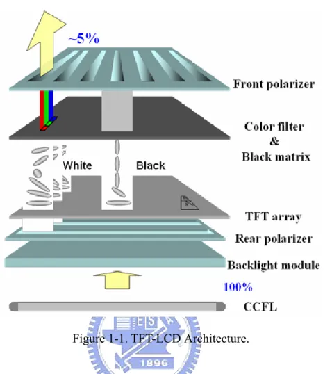
The main components of a transmissive TFT-LCD display subsystem include the video controller, frame buffer, video interface, TFT-LCD panel, and backlight. The frame buffer is a portion of memory used by software applications to deliver video data to the video controller. The video data, which is received from the processing unit, is first saved into the frame buffer memory by the video controller and is subsequently transmitted to the LCD controller through an appropriate analog (VGA) or digital (Digital Video Interface -- DVI) interface.

The video interface carries the video signals between the video controller and the TFT-LCD display. The TFT-LCD display receives the video data and generates proper transmittance for each pixel according to its pixel value. All of the pixels on the transmissive LCD panel are illuminated by the backlight from behind. To the observer, if the transmittance of a displayed pixel is high, the pixel looks bright. On the other hand, a displayed pixel looks dark if its transmittance is low. If the transmittance can be adjusted to more than two different levels, then the pixels can be displayed in grayscale. If the shade can be colored as red, green, or blue by using different color filters, then pixels can be displayed in color by mixing three sub-pixels in different colors at different grayscales. In other words, the perceived brightness of a pixel is determined by its transmittance and the backlight luminous intensity. A

(13)

normally-white TFT-LCDs architecture is shown in Figure 1-1.

Figure 1-1. TFT-LCD Architecture.

Figure 1-2 shows the typical architecture of the digital LCD subsystem including the video controller/frame buffer memory and LCD controller/panel.

Figure 1-2. LCD subsystem architecture.

Figure 1-3 shows the LCD components. The data received from the video bus is used to infer timing information and respective grayscale levels. Then, this timing information is used to select the appropriate row in the LCD matrix. Next, the pixel values are converted to the

(14)

the selected row. The backlight is powered with the aid of a DC-AC converter, to provide the required illumination.

Figure 1-3. PC system and LCD component architecture.

1.2 Backlight Scaling

The concept of backlight scaling is simply dimming the backlight to conserve power consumption and to increase image quality.

Figure 1-4. Power, backlight, transmittance, and luminance.

The luminance of LCD perceived by the user is the product of the backlight luminous intensity (b) and the panel transmittance (t):

(15)

t

b

L

=

⋅

(1-1)

The power consumption of the backlight is a strong function of its output luminance. On the contrary, the power consumption of the LCD panel is almost constant so that it is independent of the panel transmittance. Therefore, we can decrease the backlight luminous intensity b to save the power consumption P. The panel transmittance t is increased accordingly such that the luminance L remains the same. In addition, higher transmittance can reduce the light leakage phenomenon of liquid crystals and increase the image quality.

Consider a pixel consisting of red, green, and blue sub-pixel. Its color is determined by the product of the backlight luminous intensity and the transmittance of each sub-pixel:

⎥

⎦

⎤

⎢

⎣

⎡

⋅

=

⎥

⎦

⎤

⎢

⎣

⎡

B G R W B G R

t

b

L

(1-2)

LR:LG:LB is the luminance ratio of red, green, and blue. For example, white is obtained at the

ratio of 3:6:1. An LCD generates different colors by changing the transmittance ratio of sub-pixels tR:tG:tB.

If the backlight module uses red, green, and blue backlight instead of a single white backlight, then the pixel color can be represented by

⎥

⎦

⎤

⎢

⎣

⎡

⎥

⎦

⎤

⎢

⎣

⎡

=

⎥

⎦

⎤

⎢

⎣

⎡

B G R B G R B G R

t

b

L

0

(1-3)

In this case, the pixel color depends on not only the transmittance ratio but also the ratio of RGB backlights bR:bG:bB. This equation can be applied to both spatial and temporal methods of

synthesizing colors.

(16)

Most displays use either spatial or temporal method to synthesize colors (Figure 1-5). The CRT and TFT-LCD monitors use the spatial method. On the 2-dimensional screen, a color pixel consists of three sub-pixels: red, green and blue. The temporal method is used by projector displays, which produce the red, green, and blue components sequentially in a very short time period such that human vision cannot perceive the separation. This method is called

field sequential display or color sequential display.

Figure 1-5. Spatial color synthesis and temporal color synthesis.

In the color sequential display, a frame is decomposed into red, green, and blue fields, which are displayed sequentially. The three fields are illuminated by the red, green, and blue backlight accordingly, while the luminance of each color is controlled by panel transmittance.

Figure 1-6. The red, green, and blue field of a frame.

Unlike the spatial method, where a pixel consists of three sub-pixels, in a color sequential display, the RGB components of a pixel share the same estate on panel. Therefore, the pixel

(17)

density of a color sequential display can be increased to three times, which translates into 3 times display resolution (i.e., smaller pixel pitch for finer images) or 1/3 display size (for miniature displays such as head-mounted displays). The color sequential technology has been widely used in projection displays based on either the digital light processor (DLP) or LCD technology.

1.4 Motivation and Objective

The backlight dominates the power consumption of an LCD system. Our goal is to reduce the power consumption of the LCD backlight. The battery lifetime of mobile electronic devices can be prolonged. The technique, backlight scaling is used to reduce the power consumption of LCD backlight.

This scaling requires an algorithm to process. Using Brute-force algorithm in backlight scaling is a conventional method to save power consumption, but it reduces brightness, and thus, the display quality is degraded. Our objective is to dim the backlight intensity without sacrificing the visual quality. To achieve the maximum power savings for a given color distortion limit, we propose algorithms of backlight scaling for minimizing power consumption of LED backlights.

1.5 Organization

This thesis is organized as follows. The previous works and the features of backlight scaling will be presented in Chapter 2. In Chapter 3, the principles including photometric definitions, colorimetry, color appearance terminology and psychophysics will be discussed. In Chapter 4, two psychophysical experiments and experimental results will be described. The proposed algorithm of backlight scaling will be introduced in Chapter 5. In Chapter 6, the fabrication of experimental platform and measurement equipments will be illustrated. The

(18)

experimental results will be shown in Chapter 7. Finally, the conclusion of the thesis and the future work are given in Chapter 8.

(19)

Chapter 2 Previous Works of Backlight Management

In this chapter the previous works of backlight management are summarized.

2.1 Summary

Backlight scaling is by far the most effective technique for reducing power consumption in a transmissive display. This technique scales down the backlight luminous intensity to save power consumption at the cost of reduced image luminance, which results in lower visual quality. To compensate for the visual quality loss due to reduced luminance, proper image enhancement is necessary.

(a) (b)

(c) (d)

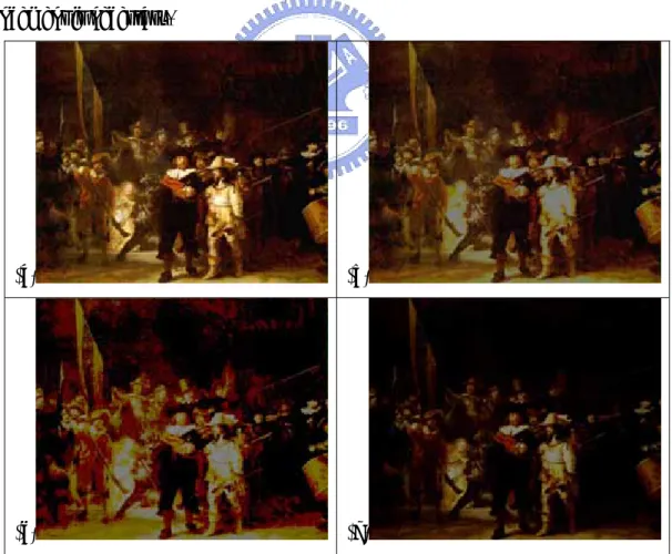
Figure 2-1. Night Watch (a) Rembrandt (b) Choi (c) Iranli (d) Cheng.

(20)

scaling have been proposed in the past years. Choi et al. proposed a technique that increases the pixel values (t) to recover the original luminance (L) [7]. However, the transmittance t in Equation 1-1 is bounded by 0 and 1. When t needs to be greater than 1, the original luminance can not be recovered and image distortion occurs. Choi’s algorithm can preserve the luminance of the dark regions, but the bright regions will be over-saturated. In their work, the number of over-saturated pixels was chosen to evaluate the image quality loss. Apparently the approach of preserving luminance L is too conservative, so preserving alternative objectives, such as a transformation on the luminance, L*=f(L), have been proposed by the other groups [13]. In addition, a series of studies were proposed in [14][15][16][17]. All of their algorithm used the same image-enhancement method for preserving luminance and restrict to image quality loss by the different conditions. They implemented their algorithm by a server and network.

Iranli et al. proposed using histogram equalization, an image processing algorithm that balances the number of pixels on each graylevel, to perform the image enhancement [12]. The transformation is the cumulative distribution function of the histogram. Histogram equalization can reproduce each graylevel distinctly without over-saturation or under-saturation. However, the proportional difference between bright and dark regions, i.e.,

tonality, will be distorted greatly when the original histogram tends to be irregular. Figure 2-1

shows such an example.

While the other researchers treat the backlight scaling problem in the brightness domain (pixel values), the same authors proposed another work that emphasizes on the mapping between luminance and brightness, commonly referred as gamma correction [18]. Gamma correction is one of the standard features for modern displays such that the end users can adjust their monitors for different viewing condition, user preferences, manufacturing variations, and luminance/color degradation as aging.

(21)

the contrast [10]. The following linear transformation was used:

⎥

⎦

⎤

⎢

⎣

⎡

−

=

⎥

⎦

⎤

⎢

⎣

⎡

gl

L

gl

L

gl

L

c

L

B G R B G R * * * (2-1)

Although Cheng’s algorithm is a compromise between preserving the brightness and preserving the contrast, it does preserve the original tonality. The relationship between brightness and contrast, however, was employed without substantial support.

The visual effects of different image enhancement algorithms are shown in Figure 2-1. The original image with 100% backlighting is shown in Figure 2-1a, in which most pixels are either very bright or very dark. Figure 2-1 show Choi’s, Iranli’s, and Cheng’s results with backlight scaled to 50%.

The minimal perceivable radiant flux from a display was calculated from the aspect of human factors by Zhong et al. in [19]. The authors concluded that the comfortable reading luminance is seven orders of magnitude larger than the just-perceptible threshold. However, such pure radiometric calculation is oversimplified without considering the other dominating human vision factors such as light adaptation and dark adaptation [20]. For example, for the classical just-noticeable difference (JND) data to be valid, the ambient light cannot be ignored, since the adaptation mechanism of human eyes can change visual sensitivity by five orders of magnitude.

In a nutshell, the principle of backlight scaling is to trade perceived image quality for power savings.In our work, we employ the results and methods that were well established in vision study, color science, psychophysical experiments to design our proposed backlight scaling algorithm.

(22)

Chapter 3 Principle: Assess Visual Quality

The research of backlight scaling involves photometry, colorimetry, psychophysics, etc. The key concepts and terminologies are reviewed in this section.

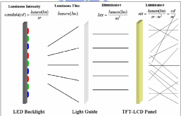
3.1 Photometric Definitions

Though light is a form of electromagnetic radiation, measurement of luminous intensity from a light source requires extra information about the relative sensitivity of the human eye to different wavelengths. Photometry is the science of measurement of the intensity of visible light and its illuminating power according to the sensitivity of the human eye. The following photometric quantities are illustrated around a TFT-LCD display in Figure 3-1.

Figure 3-1. Illustration of LED backlight and photometric terms.

Luminous flux (lumen): is the emission rate of light energy corrected for the standardized

(23)

Luminous intensity (candela): is defined as cd=lm/sr, one lumen of luminous flux per

steradiam (unit of solid angle). Luminous intensity can be used to characterize the optical power emitted from a spot light source, such as a light bulb.

Illuminance (lux): is defined as one lumen of luminous flux per area (lm/m2). Illuminance can be used to characterize the luminous power emitted from a surface. Most light meters (e.g., for photographic purpose) measure the illuminance quantity. The luminous flux may not travel in parallel after passing the surface, so that the light intensity decreases as the travel distance increases.

Luminance (nit) is physical measure, and defined as lumen per area per steradiam (lm/m2 /sr

or _cd_{/ m}2_{) [10][20].}

Luminance is used to rate the maximum brightness of CRT or LCD monitors. We use backlight factor to express the percentage of the backlight illumination, and transmissivity to express the transparency of the TFT-LCD. The backlight factor and TFT-LCD transmissivity determine the perceived luminance from the TFT-LCD display.

3.2 Colorimetry

The human eyes have three types of cones perceiving light at different wavelengths. The

L-, M-, and S-cones respond to, roughly, the wavelengths of red, green, and blue – the primaries. Mixing the three primaries in different ratios generates different colors. The colors

can be ordered in different ways and be represented by different color spaces. Computers use the RGB color space, which is convenient for the graphics adaptor and displays. Printers use the CMY color space or its variation. In color science, a color space usually consists of the one-dimensional luminance and the two-dimensional chromaticity. For a color, luminance indicates its magnitude, while chromaticity indicates the ratio between red, green and blue.

(24)

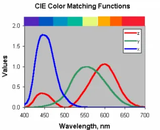
the observer, illuminator, viewing geometry, etc. Most de facto color spaces were defined by

CIE, the International Commission on Illumination. The CIE standard observer was defined

by standardizing the color matching functions, the response function of red (x), green (y), and blue (z) as shown in Figure 3-2.

Figure 3-2. The CIE color matching functions for the 1931 Standard Colorimetric Observer. Once the standard observer is defined, the CIEXYZ color space can be obtained by defining the X, Y, and Z values (in uppercase) as the product of spectral power distribution of the object Φ and the color matching function (x,y,z) across wavelength λ:

, ) ( ) (

∫

Φ = λ λ λ λ x d k X , ) ( ) (

∫

Φ = λ λ λ λ y d k Y . ) ( ) (

∫

Φ = λ λ λ λ z d k Z (3-1)

To separate the luminance component from chromaticity, the x, y, z values are defined as

, Z Y X X x + + = , Z Y X Y y + + = . Z Y X Z z + + = (3-2)

(25)

chromaticity coordinate can always be obtained from the other two by noting that the three always sum to unity. Thus z can be calculated from x and y using Equation (3-3.

y x

z= 01. − − _(3-3)

The x, y, and z value represent chromaticity, the ratio between red, green, and blue, which is independent of luminance. The z value is redundant because it can be obtained from

x and y. The two-dimensional chromaticity diagram of CIEXYZ is shown in Figure 3-3. The

horseshoe shape depicts the range of visible colors. The Euclidean distance between two different colors can be used to measure their color difference. However, CIEXYZ is not an ideal color space because the color difference is not perceived uniformly. For example, for the same color difference, a pair of blue colors is perceived more differently than a pair of green colors.

Figure 3-3. The CIE x,y chromaticity diagram. A more uniform color space, CIELAB, is defined by

, 16 ) ( 116 13 *₌ ₋ n Y Y L , ) ( ) ( 500 13 13 * ⎟⎟ ⎠ ⎞ ⎜⎜ ⎝ ⎛ − = n n Y Y X X a . ) ( ) ( 200 13 13 * ⎟⎟ ⎠ ⎞ ⎜⎜ ⎝ ⎛ − = n n Z Z Y Y b (3-4)

(26)

The CIELAB * ab

E

∆ color difference is defined by

. ) ( *2 *2 *2 * _L _a _b E_ab = ∆ +∆ +∆ ∆ (3-5) The * ab E

∆ color difference is considered as a uniform metric and has been widely used and implemented in commercial colorimeters.

Figure 3-4. CIE-Lab chromaticity diagram.

3.3 Color Appearance Terminology

The following definitions introduced in this chapter have been culled from the International Lighting Vocabulary [20].

Brightness: attribute of a visual sensation according to which an area appears to emit amore or

less light.

Lightness: the brightness of an area judged relative to the brightness of a similarly illuminated

area that appears to be white or highly transmitting.

Besides, another very important concept is contrast. The following definitions are adopted from Fairchild [22]. There are two different definitions for contrast. One definition for contrast, which is used in tone reproduction, is the rate of change of the relative luminance of image elements of a reproduction as a function of the relative luminance of the same image elements of the original image. On log-log coordinates, the contrast is the slope of the relationship between the reproduction and original. The contrast defined in this way is an

(27)

attribute of the system transfer function.

Another definition for contrast, which is used in visual science, is the difference between minimum and maximum luminance in an image. This contrast is an attribute of the image. The perceived image contrast is the perceived lightness difference between dark part and the light part of an image.

3.4 Psychophysics

Psychophysics is the scientific study of the relationships between the physical

measurements of stimuli and the sensations and perceptions that those stimuli evoke. Psychophysics can be considered a discipline of science similar to the more traditional disciplines such as physics, chemistry, and biology.

The tools of psychophysics are used to derive quantitative measures of perceptual phenomena that are often considered subjective. It is important to note that the results of properly designed psychophysical experiments are just as objective and quantitative as the measurement of length with a ruler or any other physical measurement. One important difference is that the uncertainties associated with psychophysical measurements tend to be significantly larger than those of physical measurements. However, the results are equally useful and meaningful as long as those uncertainties are considered as they always should be for physical measurements as well. Psychophysics is used to study all dimensions of human perception.

In our work, two threshold techniques proposed by Fechner were used [22][23]. The threshold experiments were designed to determine the just-perceptible change in a stimulus, sometimes referred to as a just-noticeable difference, which is used to measure the observers’ sensitivity to changes in a given stimulus. Absolute thresholds are defined as the just-perceptible difference for a change from no stimulus, while difference thresholds

(28)

represent the just-perceptible difference from a particular stimulus level greater than zero.

3.4.1 Method of Adjustment

The method of adjustment is the simplest and most straightforward technique for deriving threshold data. In this method, the observer controls the stimulus magnitude and adjusts it to a point that is just visible. The threshold is taken to be the average setting across a number of trials by one or more observers.

3.4.2 Method of Limits

The method of limits is only slightly more complex than the method of adjustment. With this method, the experimenter presents the stimuli at predefined discrete intensity levels in either ascending or descending series. In the ascending series, the experimenter presents a stimulus, beginning with one that is certain to be imperceptible, and asks the observers to respond ‘yes’ if they perceive it and ‘no’ if they do not. If they respond ‘no’, the experimenter increases the stimulus intensity. The descending series begins with a stimulus intensity that is clearly perceptible and continues until the observers respond ‘no’, they cannot perceive the stimulus. The threshold is taken to be the average stimulus intensity at which the transition from ‘no’ to ‘yes’ responses occurs for a number of ascending and descending series.

3.5 Stevens Effect

According to the classic psychophysical brightness scaling experiment from Stevens, perceived brightness could be expressed as power function of physical luminance [24].

β

ψ

=

k

(

L

−

L

₀

)

_(3-6)

where k is a constant, β is brightness (psychological magnitude), L is luminance, L0 is the

(29)

adaptation. The exponent β increases from 0.33 for the dark-adapted eye to 0.44 for the eye adapted to 1 lambert.

Furthermore, in J. C. Stevens and S. S. Stevens’ study, observers were asked to perform magnitude estimations on the brightness of stimuli across various adapting conditions. The results illustrated that the relationship between perceived brightness and measured luminance tended to follow a power function.

Figure 3-5. Results of determining the brightness functions under different states of adaptation [24].

A relationship that follows a power function when plotted on linear coordinates becomes a straight line on log-log coordinates, and shows in Figure 3-6. The Stevens effect indicates that, as the luminance level increases, dark colors will appear darker and light colors will appear lighter. While Stevens effect was demonstrated by viewing an image at high and low luminance levels, a black-and-white image is particularly effective for this demonstration. At a low luminance level, the image will appear of rather low contrast. White areas will not appear very bright, and the dark areas will not appear very dark. If the image is then moved to a significantly higher level of illumination, white areas appear substantially brighter and dark areas darker, it meant the perceived contrast has increased.

(30)

Figure 3-6. Change in lightness contrast as function of adapting luminance according to the Stevens effect [25].

3.6 Bartleson-Breneman Effect

Bartleson and Breneman conducted psychophysical experiments to investigate the perceived contrast of elements in complex stimuli (images) and how it varied with luminance level and surround [26]. Their experimental results were similar to those described by the Stevens effect with respect to luminance changes. They also observed some interesting results with respect to changes in the relative luminance of an image’s surround.

Figure 3-7. Changes in lightness contrast as a function of surround relative luminance according to the results of Bartleson and Breneman [22][29].

(31)

Their experimental results, obtained through matching and scaling experiments, showed that the perceived contrast of images increased when the image surround was changed from dark to dim to light. This effect occurs because the dark surround of an image causes areas to appear lighter while having little effect on light areas. Thus, since there is more of a perceived change in the dark areas of an image than in the light areas, there is a resultant change in perceived contrast.

(32)

Chapter 4 Psychophysical Experiments

4.1 Objective and Background

In Chapter 3, two well-known visual phenomena are introduced. They both are associated with contrast. The Stevens’ effect predicts that the perceived contrast of a simple stimulus (e.g. color) increases with the surround illumination [24]. The Bartleson-Breneman effect predicts that the perceived contrast of complex stimuli (e.g. an image) increases with the surround illumination [26]. Recently, the relationship between image contrast and surround illumination was studied by Liu [27]. However, the interaction between brightness and apparent contrast of complex stimuli has not been investigated yet.

The goal of this study is to establish the relation between perceived brightness and apparent contrast of natural images, and apply the results to display designs such as power minimization of transmissive TFT-LCDs. Our objective is to answer the following question: When the brightness of an image is reduced, can we compensate for it by increasing its contrast? If the answer is positive, then this concept can be used in low-power applications.

In this study, psychophysical experiments were employed to find the answer of the question. The psychophysical experiment consists of two steps. In the first step, the sinusoidal grating pattern was equipped for validating the interaction between perceived contrast and brightness. Furthermore, the complex stimuli were used to explore the same approach.

4.2 Perceived Brightness versus Contrast in Sinusoidal Grating Pattern

The psychophysical experiments were conducted in a dedicated darkroom. The experimental setup and apparatus are shown in Figure 4-1. A 17” CRT monitor (Viewsonic

(33)

E71f ) was used to display the sinusoidal grating patterns, which were generated by MATLAB. The resolution of the CRT is 1024×768, and the sinusoidal grating pattern in center of the display is 256×256. The distance between the observer and the monitor is 150cm.

Figure 4-1. The experimental apparatus.

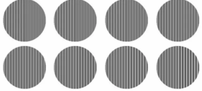
The sinusoidal grating pattern, which had 1.6 circles per degree (CPD), was vertically divided into two parts as left-hand side and right-hand side. The pattern of left-hand side presented the original pattern, which had reduced brightness; the right-hand side one presented the contrast-enhanced pattern. However, the patterns of both sides can be switched randomly for the purpose of psychophysical experiments, which are shown inFigure 4-2.

Figure 4-2. The sinusoidal grating pattern with varied apparent brightness and contrast. We used method of adjustment, a classical psychophysical method [23]. The original pattern was reduced brightness from 100% to 60%. The experiment was divided into eight trials. Each trial consists of a series of differently contrast-enhanced patterns according to reduced brightness of the original pattern. If the variation of contrast enhanced patterns was

(34)

contrast-enhanced pattern was limited to 200%. Each observer was asked to compare the original pattern against a series of differently contrast-enhanced patterns, and to find the most resemble one. In order to avoid the observer guessing the resemble pattern, the patterns of right-hand side and left-hand side were switched randomly. It meant the original pattern and contrast-enhanced pattern were not fixed on the same side.

Four observers were enlisted as subjects in the experiments. They were Asian male, aged from 23 to 29, and have normal vision after lens correction. Before starting the experiments, the subjects were asked to adapt the surround illumination for 30 seconds. Figure 4-3 shows the experimental results of four subjects as contrast vs. related brightness in the eight trials. Each curve represents an individual observer. All curves show the same tendency. This tendency points out the subjects agreed on the same isoluminance point under increasing contrast while the brightness was reduced. However, we were specifically interested in the region of brightness between 0.7 and 0.9. The experimental results show the relation between the contrast-enhancement and related brightness is close to linear in this region. The results indicate the subjects had similar perception while they viewed the two sinusoidal patterns -- one without adjustment and the other with reduced brightness and enhanced contrast -- in a specific region. Thus, the interaction between the apparent contrast and brightness is validated.

(35)

0.6 0.7 0.8 0.9 1.0 0.6 0.8 1.0 1.2 1.4 1.6 1.8 2.0 C ont rast Related Brightness Corey Geoff Andy May

Figure 4-3. Contrast versus related luminance.

4.3 Perceived Brightness versus Perceived Contrast in Complex Stimuli

In this study, we investigated the relationship between perceived image brightness and contrast by conducting psychophysical experiments. Thirty-seven observers were enlisted to perform visual experiments of determining the optimal contrast enhancement with reduced brightness.

4.3.1 Darkroom and Apparatus

The experiments were conducted in a light-proof darkroom, in which the measurable illumination is less than 0.03 lx (cf. Figure 4-4).

(36)

Figure 4-4. The setup of darkroom.

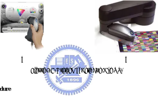
A set of six identical LED lights were installed for controlling the surround illumination. Each LED light contains three channels -- red, green, and blue. The luminance and chromaticity of the six LED lights can be controlled freely (cf. Figure 4-5). The surround illumination was projected on a white screen as the field of view. A pair of identical transmissive 19” TFT-LCD monitors (Viewsonic VX912) was used to display the test images (cf. Figure 4-6). They were driven by the same computer, and color-corrected by a GretagMacBeth Eye-One XT spectrophotometer (cf. Figure 4-7).

(a) LED light. (b) The LED lights project white surround.

(37)

Figure 4-6. TFT-LCD monitors used in the experiments.

a b

Figure 4-7. GretagMacBeth Eye-One XT.

4.3.2 Procedure

The psychophysical experiments were performed for three different levels of surround – 0%, 50%, and 100% of the full luminance of the monitors. The test image was chosen from a popular set of benchmark images from the HDR research community (www.devevec.org). The original softcopy was displayed by the left-hand-side monitor with 100% of backlighting. The contrast-adjusted softcopy was displayed by the right-hand-side monitor with 70% of backlighting. The adjusted image was displayed on the right with 70% of backlight intensity after the following contrast enhancement

255 / 126 }, 0 }, ) ( , 1 { , 0 { − + =

= MAX MIN p m slope m m

pL L (4-1)

Most of the thirty-seven observers were Asian male, aged from 22 to 28, and have normal vision after lens correction. The subjects were screened by a simple Ishihara Color

(38)

Deficiency Test, and two of them were excluded based on the test results.

Figure 4-8. Matching the original softcopy (left) with the contrast-adjusted one (right). The experiment started with a 30 seconds period for the subject to adapt to the surround illumination while the monitors displayed gray fields of the same luminance. The subject was asked to match the original softcopy with the contrast-adjusted one (cf. Figure 4-8). The classical psychophysical method, Method of Limits [23], was used. A series of differently contrast-enhanced images in ascending/descending order was displayed sequentially (cf. Figure 4-9).

Figure 4-9. The image contrast was modulated between high (left) and low (right). The subject had to decide if the point of isoluminance was reached. The corresponding contrast adjustment at the point of isoluminance was recorded for analysis. The experiments were repeated for three times with surround at 0%, 50%, and 100%.

4.3.3 Experimental Results

Figure 4-10 shows the experimental data as subject count vs. contrast adjustment in the ascending and descending trials. The top/bottom curve represents the descending/ascending

(39)

data. Each point indicates the number of subjects who agreed on the same isoluminance point. Both ascending and descending distributions are near Gaussian with a mean value around 120% contrast-adjustment. It indicates that most subjects agreed on this point of isoluminance. The mean of the ascending trial is greater than that of the descending trial. The reason is the persistence of visual perception, which is common in experiments using Method of Limits. 0 1 2 3 4 5 -2 0 2 4 6 8 10 12 14 16 18 Count Contrast Descending Ascending

Figure 4-10. Subject count vs. contrast adjustment for ascending (bottom) and descending (top) trials.

4.4 Summary

According to the experimental results, decreased brightness can be compensated by increasing luminance contrast. The experimental results can be applied to low-power display design. In a transmissive TFT-LCD, reducing the backlight intensity to save power consumption, at the cost of degraded image quality, is a common practice. Based on our findings, one can increase the contrast to recover the image quality.

(40)

same image. The relation between image quality and contrast enhancement is shown in Figure 4-11.

Figure 4-11. Contrast fidelity vs. contrast.

We found high resemblance between Figure 4-10 and Figure 4-11. In other words, for the given image, our psychophysical findings are in accordance with the analytical model in [10]. Although further experiments are undergoing for more concrete conclusions, in this work we adopted the CBCS algorithm.

(41)

Chapter 5 Proposed Algorithm

We propose a backlight scaling algorithm for an LED backlit display. The proposed algorithm consists of two phases. In the first phase, chromaticity scaling, the image is chromatically scaled subject to the perceivable colorfulness difference. The optimal ratio of RGB backlights is found to achieve maximum power savings at the same luminance. In the second phase, luminance scaling, the luminance is scaled down to achieve maximum power savings subject to the perceivable lightness difference.

5.1 Chromaticity Scaling

Figure 5-1. Photo and R, G, and B histogram.

The motivation of chromaticity scaling is that most images have different distributions in their RGB histograms. To achieve more power savings, the RGB channels can be scaled differently. For example, in Figure 5-1, in average the red channel has higher luminance than the blue channel does. This observation implies that the blue backlight can be scaled down more than the red backlight. However, the side effect of scaling RGB channels differently is color shift. Therefore, we use the color difference defined by Equation (3-5) to govern the chromaticity scaling. We define the following notation to represent an image after

(42)

chromaticity scaling.

⎩

⎨

⎧

>

≤

=

≡

_∈ i i i i i i B G R i B G R

_p

_b

b

p

b

p

b

I

,

)

,

(

_{ _, _, _} _(5-1)

When the red, green, and blue backlight are down-scaled from 1.0 to bR, bG, and bB

respectively, the red, green, and blue sub-pixel will be clipped by bR, bG, and bB respectively.

We use ∆E(I1, I2) to indicate the average color difference between the original image I1 and

chromaticity-scaled image I2. Given Q as the color shift constraint, the following algorithm

finds the optimal chromaticity scaling factors that save the most power consumption with the least color shift. The procedure of finding backlight factor shows in Figure 5-2.

Chromaticity_Scaling: ); ( / )) , , ( ), 1 , 1 , 1 ( ( ); ( / )) , , ( ), 1 , 1 , 1 ( ( ); ( / )) , , ( ), 1 , 1 , 1 ( ( * * * δ δ δ δ δ δ − − ∆ = − − ∆ = − − ∆ = B B B G R ab B G G B G R ab G R R B G R ab R b P b b b I I E S b P b b b I I E S b P b b b I I E S

Find MIN(SR,SG,SB), whose ∆Eab ≤Q

* ;

if (found) then

Depend onMIN(SR,SG,SB), update either bR, bG, or bB with bR－δ, bG－δ, or bB－δ

accordingly;

goto Chromaticity_Scaling; else

(43)

Figure 5-2. Procedure of finding backlight factor. 5.2Luminance Scaling

The original CBCS algorithm [10] is used in the second phase. The affined linear transformation of a pixel pL can be parameterized by

, , ), ( , 0 ) , , 0 , ( * L L L L L L L p gu gu p gl gl p b gl p c p b gu gl CBCS < ≤ ≤ < ⎪ ⎩ ⎪ ⎨ ⎧ − = ≡ _(5-2)

where bL is the backlight factor and

. gl gu b c L − = _(5-3)

The image quality is defined by

),

(

)

(

x

PDF

x

f

F

gu gl c C

=

∑

(5-4) where

(44)

0, 0 , , 0 1 0, 1 ( ) x gl c gl x gu c c gu x f x ⎧ ≤ < ⎪ _{≤ ≤} _{≤ ≤} ⎨ ⎪ _{< ≤} ⎩ = (5-5)

and PDF(x) is the probability density function of pixel value x. The RGB backlights are scaled simultaneously by a factor bL such that no more color shift will be introduced. Since

the ratio between the RGB is fixed, this phase is called luminance scaling. The following LED power equation is used.

P

R

(b

L

b

R

)+P

G

(b

L

b

G

)+P

B

(b

L

b

B

)

(5-6)

The objective function is to find the optimal gl, gu, and bL that minimize Equation (5-6)

subject to the given image quality constraint FC.

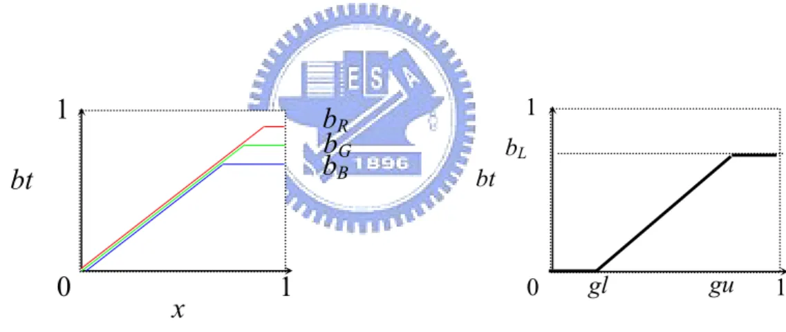
Sample transfer functions of chromaticity and luminance scaling are shown in Figure 5-3.

Figure 5-3. Transfer functions of chromaticity and luminance scaling. 5.3 Summary

In our algorithm, the chromaticity scaling is employed to find the maximum power consumption which can be saved in an image while the color difference ∆E is determined. We reduce the backlight intensity by using the results of chromaticity scaling.

Luminance scaling uses CBCS algorithm. The transfer function changes the pixel data for compensating the luminance loss while the backlight intensity is reduced. The algorithm is the foundation that constructing a platform of the low power display.

0 x

bt

1

1 _b

R

b

G

b

B 0 bL bt 1 1 gl gu

(45)

Chapter 6 Prototype

6.1 Framework

For implementing our algorithms of backlight scaling, a prototype of experimental platform is necessary. Unfortunately, it is too difficult to get an appropriate hardware for matching the portable electronic device. Furthermore, the structure and optical mechanism of the portable electronic device can be easily shifted or damaged after the panel refitted. Therefore, it is critical to determine a prototype to overcome these difficulties.

Figure 6-1. Backlight scaling of portable electronic device.

The design of our prototype is changed from the portable electronic device system (small size panel) to the laptop computer system (large size panel) through the support of CPT Corporation. Because our purpose is to reduce the power consumption of the TFT-LCD backlight, this switch has no influence on our implementation. There are several benefits in this switch. A ready hardware (FPGA board) from the support of CPT Corporation can be used to design this prototype. Refitting the large size panel is easier than refitting the small ones for us. Moreover, for a panel manufacturer, they can apply the technology of large size

(46)

panel to the small size panel readily. The power consumption of the LCD backlight can be measured more conveniently.

In our framework, the backlight scaling algorithm is realized in a Field Programmable Gate Array (FPGA) board. The FPGA board is used for image processing and backlight controller, which connects the TFT-LCD and the personal computer. The TFT-LCD displays the images before/after the backlight scaling process with the FPGA, while we measure the power consumption of TFT-LCD backlight.

Figure 6-2. Our notion of backlight scaling. 6.1.1 Image Processing Flow

In image data processing flow of the personal computer, first, the image data is stored in the frame buffer by the CPU, and then graphic card fetches this image data and generates appropriate analog or digital image data to the video interface. The image data is carried by VGA or DVI interface and delivered to the scaler board.

According to the panel characteristic, the scaler board automatically scales the image data to appropriate frame resolution and frame rate. Moreover, some scaler chips include extra functionality, such as video decoding, video processing and 3D graphics accelerator, etc. Finally, the image data is translated into the signal format of TTL or Low Voltage Differential Signaling (LVDS) by scaler board and is delivered to panel controller board.

(47)

Figure 6-3. Block diagram of image processing flow.

6.2 Block Diagram of Prototype

Our goals are to reduce the power consumption of the LCD backlight and to maintain the image brightness with our backlight scaling algorithms. This consideration of fetching and processing image data from the PC will be used to design the experimental platform. There are different methods available to fetch the image data; one is to fetch the image data as it is delivered by graphic card, and another is to fetch the image data as it passes the scaler board.

It is more complex to process image data with the first method. Furthermore, some scaler boards include the functionality of image processing. While the image data passes the scaler board, the image data is probably adjusted or changed by scaler board. Base on the above reasons, we chose the second method. Unfortunately, because of the higher resolution TFT-LCD panel, the image data is translated into LVDS signal format by the scaler board while the image data passes the scaler board. LVDS signal format will complicate the image

(48)

fetching and processing.

Figure 6-4. Fetching the image data as the image data is delivered by graphic card.

Figure 6-5. Fetching the image data as the image data passes the scaler board. 6.2.1 Low Voltage Differential Signaling

(49)

performance data transmission applications. The LVDS standard is becoming the most popular differential data transmission standard in the industry.

In the TFT-LCD field, the LVDS standard is usually used in the signal transmission of the higher-resolution LCD because it requires more data flow than low-resolution LCD.

LVDS delivers high data rates while consuming significantly less power than competing technologies. In addition, it brings many other benefits, which include:

• Low-voltage power supply compatibility • Low noise generation

• High noise rejection

• Robust transmission signals

• Ability to be integrated into system level ICs

LVDS technology allows products to address high data rates ranging from 100’s of Mbps to greater than 2 Gbps. For all of the above reasons, it has been deployed across many market segments wherever the need of speed and low power exists.

Figure 6-6. Simplified diagram of LVDS driver and receiver.

LVDS is a low swing, differential signaling technology, which allows single channel data transmission at hundreds or even thousands of megabits per second (Mbps). Its low swing and

(50)

a wide range of frequencies.

LVDS outputs consist of a current source (nominal 3.5 mA) that drives the differential pair lines. The basic receiver has a high DC input impedance, so the majority of driver current flows across the 100Ω termination resistor generating about 350 mV across the receiver inputs. When the driver switches, it changes the direction of current flow across the resistor, thereby creating a valid “one” or “zero” logic state.

6.3 Platform

6.3.1 Experimental Panel

The experimental panel is equipped with a 1280×1024, 19”, 24-bit color, transmissive, color TFT-LCD monitor, ViewSonic VX912.

In our work, LED was used to fabricate backlight module. The backlight scaling panel and backlight was evaluated by a conventional TFT-LCD monitor. The prototype was built on a VX912 monitor. Originally the LCD panel has two side-lit CCFL backlights on the top and bottom. We custom made two LED backlights to replace the CCFL backlights.

(51)

The display panel manufactured by AUO Corporation includes a major application specific integrated circuit (ASIC) and an SXGA TFT-LCD panel [30]. The image data feeds into the AUO ASIC, which includes the timing controller and RSDS transmitter. The connector receives the LVDS signal which is from the scaler board, and then delivers to the AUO ASIC. The LVDS signal is translated into RSDS by the AUO ASIC, and then delivers to TFT-LCD.

Figure 6-8. Block diagram of the AUOpanel.

6.3.2 FPGA Board

In the beginning, we implement the panel controller and backlight controller with an FPGA board which is supplied by CPT Corporation and Xilinx Spartan-3 Starter Kit [31], respectively. The CPT FPGA board includes an LVDS transmitter and receiver, and an FPGA chip. The Xilinx Spartan-3 starter kit houses 200,000-gate Xilinx Spartan-3 XC3S200 FPGA in a 256-ball thin ball grid array package (XC3S200FT256), 2Mbit Xilinx XCF02S platform flash, in-system programmable configuration PROM, 1M-byte of fast asynchronous SRAM, 3-bit, 8-color VGA display port, 9-pin RS-232 serial port, 50 MHz oscillator, and several I/O ports.

(52)

Figure 6-9. Xilinx Spartan-3 Starter Kit Board [31].

The CPT FPGA board includes three major ports; they are LVDS receiver, FPGA chip, and LVDS transmitter. The function of the LVDS receiver is to translate the LVDS signal format of image data to TTL signal format. Next, the TTL signal is delivered to the FPGA chip.

Our backlight scaling algorithm was programmed in HDL code, and then written into the FPGA chip. The TTL signal format of image data is processed by the FPGA chip, and then translated into LVDS signal format through the LVDS transmitter.

6.3.3 LED backlight

Our prototype LED backlight uses top-emitting LED chips. Each LED chip houses four LEDs – one red, two green in series, and one blue. The 1:2:1 ratio was determined by chromatic sensitivity and device efficiency. The three colors were driven separately such that the output chromaticity can be adjusted.

The LED backlights were used to replace the CCFL backlights of the VX912. Each LED backlight consists of 24 LED chips, wired as 4 parallel sets of 6 serial chips. Each channel is driven by a dedicated current mirror driver on a custom designed PCB. The driving current is controlled by a pulse-width modulation (PWM) signal.

(53)

Figure 6-10. LED and LED backlight.

Figure 6-11. Block diagram of backlight module.

Figure 6-12. LED backlight driving board.

6.3.4 Instruments and Equipment

The color and brightness of image are the most important properties of a systemthat we want to evaluate. The chroma meter (Konica-Minolta chroma meter CS-200) was used to measure these properties. It utilizes three high-sensitivity silicon photo-cells, which are filtered to match the CIE standard observer response. It can be used to measure various chromaticity coordinates by calculating three measurements, such as Lxy, Luv, Lu’v’, dominant wavelength, color temperature, etc. With this compact, reliable color analyzer, we

(54)

can easily get the chromaticity coordinates and luminance of the displayed image. The chroma meter CS-200 was also used to calibrate the white point of our prototype.

The programmable power supplies, GW PPT-3615, were used to support the LED

driving board and LED backlights power. The digital multimeters, GDM 8246, were used to measure the current of LED backlights. We can obtain the voltage data of the LED backlights from the power supplies, and also obtain the current data from the multimeters. The power consumption can be calculated as the product of the voltage and current.

Figure 6-13. Chroma meter. Figure 6-14. Power supply. Figure 6-15. Multimeter.

6.3.5 Platform Block Diagram

In the final block diagram, we combined the backlight controller and panel controller onto the CPT FPGA board. The algorithm was also implemented in VHDL, the CPT FPGA Board. The following block diagrams are illustrated around the experimental setup in Figure 6-16.

z PC: Generating the image signals for the scaler board.

z Scaler Board: Scaling the image data to appropriate frame resolution and frame rate where the image signal is LVDS format.

z FPGA Board: Receiving LVDS signals and then translating signal to the TTL format. Furthermore, performing the proposed algorithm image processing, and then outputting the VGA signal to drive the 19” TFT-LCD panel. At the same time, The FPGA board also generates the pulse width modulators (PWM) to control the

(55)

backlight intensity of the RGB channels.

z Multimeter: Measuring the driving current of the LEDs. z Power Supply: Powering LED and their drivers.

z LED Driver: Driving the LEDs.

Figure 6-16. Layout of experimental system.

6.4 FPGA Architecture

The critical component of our experimental platform is the CPT FPGA board. The algorithm of backlight scaling is programmed with very high speed integrated circuit hardware description language (VHDL) code and then writes into the FPGA chip, which is on the CPT FPGA board. The two major assignments are executed by FPGA chip adjust the image data from the scaler board and adjust the backlight intensity.

6.4.1 Display Signal

(56)

on an afterimage of human eyes. As we reduce the refresh rate of the CRT display that exceeds the minimum period for an afterimage on the human eye, we start to feel flicker. In other words, the image on the CRT display is always flickering; but human eyes do not recognize it as long as the flickering frequency is high enough. Meanwhile, the image on the TFT LCD panel also flickers, but the flicker on the LCD panel is of a different nature. As far as the refresh rate is higher than the time constant of the storage capacitors, the image on the LCD display does not flicker at all. Consequently, we can reduce the refresh rate of the LCD display as long as it is shorter than the time constant of the storage capacitors. Actually, modern LCD displays adopt flicker free techniques, and the time constant is much longer than that of the CRT display. In addition, as we increase the refresh rate of the CRT display far exceeding the minimum period for the afterimage, we do feel better quality; so we often use 120Hz or higher refresh rate for high quality image. However, once the refresh rate is higher than the time constant of the storage capacitors, the image quality of the LCD display is not enhanced further. Therefore, most LCD panels support fixed refresh rate, unlike CRT displays.

Vertical synchronization (Vsync) is a signal used to describe the process or set a value telling the monitor when to draw the next vertical line. Vsync determines the frame frequency of the display. The frame rate of CRT display can be adjusted, but LCDs cannot, due to the LC response time is limited. So, most LCDs support fixed frame rate, unlike CRT display. Meanwhile, the frame rate of the TFT-LCDs is usually 60Hz. Horizontal synchronization (Hsync) is a signal telling the monitor to stop drawing the current horizontal line, and starts drawing the next line. Each high state of the DE (data enable) signal matches the high state of a Hsync signal.

(57)

Figure 6-17. Waveform chart of video signal (a).

The DE signal determines the data writing in the period of the high state. In the period of high state of the DE signal, which is active time and the data of an image is valid. As the DE signal is low state, the data of the image is invalid even though the Hsync is high state.

Figure 6-18. Waveform chart of video signal (b).

The DCLK means the pixel clock. Each period of the DCLK represents the transmission data of a pixel is valid and the amount of the pixels is 1280 while the DE is high state. Meanwhile, the data width is 24 bits, which means that the data width of R, G, and B of an image has 8 bits.

人眼視覺導向之低功耗液晶顯示器背光管理

國立交通大學

電機學院光電顯示科技產業研發碩士班

碩士論文

人眼視覺導向之低功耗液晶顯示器背光管理

Visual Perception-Guided Low-Power LCD

Backlight Management

研究生：趙健富

指導教授：鄭惟中 博士

人眼視覺導向之低功耗液晶顯示器背光管理

Visual Perception-Guided Low-Power LCD

Backlight Management

研 究 生: 趙健富

Student: Chien-Fu Chao

指導教授: 鄭惟中 博士 Advisor: Dr. Wei-Chung Cheng

國立交通大學

電機學院光電顯示科技產業研發碩士班

碩士論文

A Thesis

Submitted to College of Electrical and Computer Engineering

National Chiao Tung University

in Partial Fulfillment of the Requirements

for the Degree of

Master

in

Industrial Technology R & D Master Program on

Photonics and Display Technologies

February 2007

Hsinchu, Taiwan, Republic of China

人眼視覺導向之低功耗液晶顯示器背光管理

碩士研究生：趙健富 指導教授：鄭惟中 博士

國立交通大學 電機學院

中文摘要

Visual Perception-Guided Low-Power LCD

Backlight Management

Student：Chien-Fu Chao Advisor：Dr. Wei-Chung Cheng

National Chiao Tung University

ABSTRACT

致 謝

Table of Contents

List of Tables

List of Figures

Chapter 1

Introduction

t

b

L

=

⋅

⎥

⎥

⎥

⎦

⎤

⎢

⎢

⎢

⎣

⎡

⋅

=

⎥

⎥

⎥

⎦

⎤

⎢

⎢

⎢

⎣

⎡

t

t

t

b

L

L

L

⎥

⎥

指導教授：鄭惟中博士

研究生: 趙健富

指導教授: 鄭惟中博士 Advisor: Dr. Wei-Chung Cheng

碩士研究生：趙健富指導教授：鄭惟中博士

國立交通大學電機學院

致謝