National Chiao Tung University
Department of Transportation and Logistics
Management
Thesis
一個國家的物流能力是否會傳染給與其主要貿易夥伴?
從全球供應鏈管理的觀點
Is the Quality a Country’s Logistics Contagious to Its Major Trading
Partners? A Perspective from Global Supply Chain Management
Student
: Misbakhul Anam
Advisor
: Kun Feng Wu, Ph.D
Andi Cakravastia, Ph.D
一個國家的物流能力是否會傳染給與其主要貿易夥伴?從全球供應鏈管理
的視角
Is the Quality a Country’s Logistics Contagious to Its Major Trading
Partners? A Perspective from Global Supply Chain Management
研究生
: 安銘思
Student
: Misbakhul Anam
指導教授 : 吳昆峰
Andi Cakravastia
Advisor
: Kun Feng Wu
Andi Cakravastia
國立交通大學
運輸與物流管理學系
碩士論文
A Thesis
Submitted to Department of Transportation and Logistics Management College of Management
National Chiao Tung University in partial Fulfillment of the Requirements
for the Degree of Master
In
Logistics Management
August 2014
Hsinchu, Taiwan, Republic of China
一個國家的物流能力是否會傳染給與其主要貿易夥伴?從全球
供應鏈管理的視角
研究生:安銘思 指導教授:吳昆峰
Andi Cakravastia運輸與物流管理學系
國立交通大學
摘
要
一個國家的物流品質一直以來被視為一個國家競爭力的重要因素之一,所 以過去已有許多研究針對影響國家物流績效的因素進行探討。由過去研究 之成果,本研究從全球供應鏈觀點假設一個國家的貿易夥伴物流績效表現 會影響到該國的物流績效表現,並利用國與國間之貿易值來檢視本研究假 定國與國之間的空間相關性。繼而,本研究嘗試構建空間迴歸模型,主要 用以檢測控制其他影響因素下之空間效果。另外,本研究採用經由世界銀 行制定以衡量每一個國家的物流績效指數(LPI)以作為衡量一個國家服務 品質,亦針對印尼42個主要貿易夥伴,約佔印尼全年總貿易額的93%。研 究結果顯示一個國家的物流績效指數對主要貿易夥伴的物流績效表現影 響是非常顯著的。 關鍵字:全球供應鏈、物流績效指數、空間迴歸分析、空間相關、貿易額 iIs the Quality a Country’s Logistics Contagious to Its Major Trading Partners? A Perspective from Global Supply Chain Management
Student : Misbakhul Anam Advisors : Kun Feng Wu, Ph.D Andi Cakravastia, Ph.D
ABSTRACT
The quality of a country’s logistics has long been considered as one of the most important factors for a country’s competitiveness. Hence, many studies have been researching into factors influencing countries’ logistics performance. Among many of which, this study hypothesizes that the logistics performances of a country’s trading partners may play a large role in affecting the country’s logistics performance from a global supply chain perspective. This research utilizes spatial analysis to investigate the hypothetical spatial correlation in terms of countries trading values. Spatial regression models are employed to test the spatial effect while controlling for other confounding factors. This study adopts the World Bank’s Logistics Performance Index (LPI) as a measure of the quality of a country’s logistics. This study focuses on 42 Indonesia’s trading partners as all of which accounts for about 93 percent of the annual total trading value. Our results show that a country’s LPI is significantly influenced by its major trading partner’s LPI.
Key words : global supply chain, logistics performance index, spatial regression analysis, spatial
correlation, trading value
ACKNOWLEDGEMENTS
We convey our gratitude to the World Bank and World trade Organization for the data in this research. The second author is also grateful to National Chiao Tung University in Taiwan, Bandung Institute of Technology (ITB) in Indonesia, and The Ministry of Industry (MOI) of Indonesia for the support by which this piece of collaborative research could be made.
iv TABLE OF CONTENTS 摘要 ... i Abstract ... ii Acknowledgement ... iii Table of Contents ... iv List of Tables ... v List of Figures ... vi 1. INTRODUCTION ... 1 2. LITERATURE REVIEW ... 3
2.1 The Logistics Performance Index ... 3
2.2 Factors Identification ... 5
2.3 Spatial Correlation ... 6
2.4 Research Hypothesis and Design ... 7
3. METHODOLOGY ... 8
3.1 The Spatial Regression Model ... 8
3.2 The Neighborhood Design ... 11
3.3 Data ... 15
4. DATA ANALYSIS ... 16
4.1 Analyses by LPI Components ... 16
4.2 Analyses by Different Commodity ... 17
4.3 The Overall Spatial Correlation ... 19
5. CONCLUSION ... 21
REFERENCES ... 22
LIST OF TABLES
Table 1. The factors affect to LPI from literature study ... 5
Table 2. The studies analyze the factor affecting to LPI by considering spatial effect ... 6
Table 3. The result of analyses by LPI components ... 16
Table 4. The result of analyses by different commodity ... 18
LIST OF FIGURES
Figure 1. The neighbor countries coordinates based on geographical distance ... 13 Figure 2. The neighbor countries coordinates based on trading value ... 14 Figure 3. The comparison of neighbor countries coordinates based on
trading value and geographical distance ... 14 Figure 4. The comparison of spatial correlation value of sector analysis ... 19
1. INTRODUCTION
The quality of a country’s logistics has long been considered as one of the most important factors for a country’s competitiveness. Arvis (2012) proposed that the most important elements of national competitiveness is the national logistics and it plays a critical role in promoting regional and international trade. The most commonly used set of indicators for measuring logistics efficiency across countries is the World Bank’s Logistics Performance Index. Based on a survey of about conducted by one thousand logistics professionals, shows that the LPI is an index number between one and five summarizing performance in six key areas, namely efficiency of the clearance process, quality of trade and transport infrastructure, ease of arranging competitively priced shipments, competence and quality of logistics services, ability to track and trace consignments, and timeliness of shipments in reaching their destination.
Some empirical studies have also revealed factors which is related to the logistics performance. Gunner et. al (2012) found that social and government regulations such as political stability, government efficiency, control of corruption and human development index have significant relationship with the LPI. Goh and Ang (2000) mentioned that road and port infrastructure affects the logistics performance. Puertas et. al (2013) also mentioned that gross domestic products, customs, and port infrastucture have significant relationship to logistics performance as well as trading activity which also have relationship with logistics performance (Hausman, et. al, 2010).
It is indeed, in the context of global supply chain, that international trading is something that is inevitable leading to countries becoming borderless and can trade their products to one another easily and can source from the other countries for their needs which are not available within their reach. At company level, global supply chain give many advantages for the effectivity and efficiency of a company and there is a possibility of it to set up a subsidiary company, production site and warehouse in other countries courtesy of global supply chain. Moreover not all raw materials can be available to satisfy the needs of the company and in order for the company to satisfy its need in terms of raw materials would need to outsource from other countries that have it. Thus will lead to inter-state trade called international trade.
The international trading activity encourage countries to improve their logistics performance. A better logistics performance of a country ensures the effectiveness and
efficiency of international trading activity in terms of cost and time. Francois et. al (2007) stated that there are many factors related to international trade such as tax, custom, infrastructure (port and road), freight transport, and logistics service. Sheperd et. al (2011) also stated that there is an extensive evidence indicating that better trade logistics tend to boost international trade performance.
There are some studies which investigate the relationship between trading and logistics performance. This has been conducted with the consideration of spatial effect and found that a country’s logistics performance is influenced by gross domestic product (GDP) and the distance of the country. Meanwhile, Wilson et. al (2004) found that quality of port and customs affects the logistics performance. Moreover, Andersoon and Wincoop (2004) stated that freight cost and tax influence the logistics performance. Hausman et. al. (2012) found that there are negative correlation between trading value and distance. However, in real condition trading, it is not always having negative correlation to distance. Countries which have far distance may have greater trading value than other countries which are more close. For example, Indonesia’s total trading value to USA in 2012 is 26,52 million USD greater than Indonesia’s total trading value to Philippines at 4,5 million USD. Based on this data, the trading value is used as a basis to define the spatial terms instead of distance. Meanwhile, the method used in this research is spatial regression analysis which makes is possible to define the spatial terms based on trading value.
This research comes up with the hypothesis that the logistics performances of a country’s trading partners may play a large role in affecting the country’s logistics performance. The data used in this research is LPI data issued by World Bank and the Indonesia’s trading value data with 41 trading partner countries as all of which accounts for more than 93 percent of the annual total trading value.
This paper has five sections. After this introduction, section two presents literature review on logistics performance index (LPI), the factor related to LPI, and spatial correlation. Section three introduces the proposed methodology. Section four presents the data analysis. The final section is conclusion of this research and suggestions for further studies.
2. LITERATURE REVIEW
This chapter presents the literature review about the logistics performance index, identification to the factors which influencing to logistics performance, the spatial correlation, and the research hypothesis and design.
2.1 The Logistics Performance Index
The Logistics Performance Index and its indicators have been constructed from information gathered in a worldwide survey of the companies responsible for moving goods and facilitating trade around the world, the multinational freight forwarders and the main express carriers. It relies on the experience and knowledge of professionals. Their views matter: they have a direct impact on the choice of shipping routes and gateways and can influence the firms’ decisions about the location of production, choice of suppliers, and selection of target markets.
The indicators summarize the performance of countries in seven areas that capture the current logistics environment. They range from traditional areas such as customs procedures, logistics costs (such as freight rates), and infrastructure quality to new areas such as the ability to track and trace shipments, timeliness in reaching a destination, and the competence of the domestic logistics industry. None of these areas alone can ensure good logistics performance. The selection of these areas is based on the latest theoretical and empirical research, and on extensive interviews with logistics professionals involved in inter-national freight logistics. The LPI synthesizes this information in a composite index to allow for comparisons.
The LPI and its indicators are given on a numerical scale, from 1 (worst) to 5 (best). This scale can also be used to interpret performance outcomes measures. For example, the analysis based on the additional country information gathered in the survey indicates that, on average, having an LPI lower by one point (say, 2.5 rather than 3.5) implies six additional days for getting imports from the port to a firm’s warehouse and three additional days for exports. It also implies that a shipment is five times more likely to be subject to a physical inspection at entry.
To provide a more complete picture of the key factors determining logistics performance, the Logistics Performance Survey asked logistics professionals about the institutions and processes supporting logistics operations in the countries in which they
are based. It asked them to assess critical attributes of the supply chain, including timeliness of deliveries, quality of transport and IT infrastructure, efficiency of border clearance processes, competence of the local logistics industry, and domestic costs of services as well as provide time and cost data.
Based on the world bank report on LPI survey (2012) the indcator questions in the logistics performance survey delved into the quality of infrastructure, the competence of private and public logistics service providers, the roles of customs and other border agencies, such governance issues as corruption and transparency, and the reliability of the trading system and supply chains. Reliability (measured by the predictability of the clearance process and the timely delivery of shipments) emerged as a key concern, with the difference in satisfaction between the high-and low-performing countries much larger than for any other question in the survey.
Quality of infrastructure
The Quality of Port Infrastructure measures business executives' perception of their country's port facilities.
Competence of private and public logistics service providers
This indicator measures the performance of the supply chain depends on the quality of services delivered by the private sector through customs brokers and road transport operators and on the competence and diligence of public agencies in charge of border procedures.
Customs and other border agencies
Customs performance tends to be better than that of other border agencies; on average, customs clearance accounts for a third of import time. This underscores the importance of addressing the coordination of border agencies, especially in countries that already have attained good customs clearance.
Corruption and transparency
The transparency of government procurement, the security of property from theft and looting, macroeconomic conditions, and the underlying strength of institutions are critical factors in determining logistics performance.
Reliability of the trading system and supply chain
The reliability of the trading system and supply chain is the most important aspect of logistics performance. A high degree of uncertainty means that operators have
to adopt costly hedging strategies, such as maintaining relatively high inventory levels.
The detail information about the indicator questions in the logistics performance survey can be seen in Appendix 1.
2.2 Factors Identification
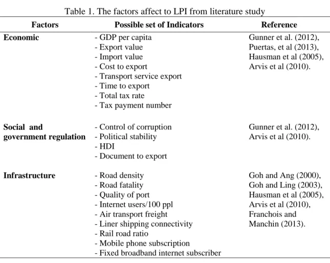
The previous studies have been conducted to analyze the factors that have relation to the logistics performance. Some factors such as the economic, social and government regulation, and infrastructure factors are evidently have relation to logistics performance. The customs, cost and time to export are some factors that influencing to the logistics performance in regard to economic. Meanwhile, in terms of social and government regulation, political issues and quality of human resources have the relation to logistics performance. In terms of infrastructure, the quality of transportation infrastructure has the relation to the logistics performance. All factors and their reference in details are shown in Table 1.
Table 1. The factors affect to LPI from literature study
Factors Possible set of Indicators Reference
Economic - GDP per capita
- Export value - Import value - Cost to export
- Transport service export - Time to export
- Total tax rate
- Tax payment number
Gunner et al. (2012), Puertas, et al (2013), Hausman et al (2005), Arvis et al (2010). Social and government regulation - Control of corruption - Political stability - HDI - Document to export Gunner et al. (2012), Arvis et al (2010).
Infrastructure - Road density - Road fatality - Quality of port - Internet users/100 ppl - Air transport freight - Liner shipping connectivity - Rail road ratio
- Mobile phone subscription
- Fixed broadband internet subscriber
Goh and Ang (2000), Goh and Ling (2003), Hausman et al (2005), Arvis et al (2010), Franchois and Manchin (2013).
2.3 Spatial Correlation
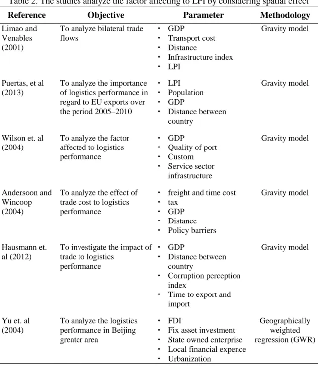
There are some studies analyzed the factors affecting logistics performance by considering spatial effect. The gravity model is the most commonly model which used in analyzing the factors that relating to the logistics performance by considering spatial effect. In addition, some studies utilized the geographically weighted regression. Table 2 presents the resume of previous studies which analyze the factor affecting to logistics performance by considering spatial effect:
Table 2. The studies analyze the factor affecting to LPI by considering spatial effect
Reference Objective Parameter Methodology
Limao and Venables (2001)
To analyze bilateral trade flows • GDP • Transport cost • Distance • Infrastructure index • LPI Gravity model Puertas, et al (2013)
To analyze the importance of logistics performance in regard to EU exports over the period 2005–2010 • LPI • Population • GDP • Distance between country Gravity model Wilson et. al (2004)
To analyze the factor affected to logistics performance • GDP • Quality of port • Custom • Service sector infrastructure Gravity model Andersoon and Wincoop (2004)
To analyze the effect of trade cost to logistics performance
• freight and time cost • tax • GDP • Distance • Policy barriers Gravity model Hausmann et. al (2012)
To investigate the impact of trade to logistics performance • GDP • Distance between country • Corruption perception index
• Time to export and import
Gravity model
Yu et. al (2004)
To analyze the logistics performance in Beijing greater area
• FDI
• Fix asset investment • State owned enterprise • Local financial expence • Urbanization
Geographically weighted regression (GWR)
Based on literature review that gravity model analysis and geographically weighted regression (GWR) were utilized to analyze the factor which affecting logistics performance by considering spatial effect. Both models are use distance in defining spatial terms. This research propose to use spatial regression analysis instead the gravity model and geographically weighted regression.
Unlike the gravity model and geographically weighted regression (GWR), which is spatial term (the neighborhood design) defined based on distance, the spatial regression analysis allow to define the neighborhood design based on other criteria instead of distance. The neighborhood design in this research defined based on total trading value, therefore the spatial regression analysis is utilized. The motivation of using trading value instead of geographical distance in defining neighborhood design is due to the fact that logistics performance have strong correlation with trading activity. The trading activity can become a stimulus for a country to improve their logistics performance. In fact, trading activity is not have linear correlation to the geographical distance, a country might have gretaer trading value with country that have further distance.
2.4 Research Hypothesis and Design
This research hypothesizes that the logistics performances of a country’s trading partners may plays a large role in affecting the country’s logistics performance from a global supply chain perspective. The research was conducted by collecting the LPI data and factors that influence it and an Indonesia’s trading value data with 41 trading partner countries. All the data were analyzed using spatial regression model to test the LPI spatial correlation. The LPI was selected as dependent variable because it provides snapshots of the supply chain performance of a country and widely accepted by almost all countries around the world.
3. METHODOLOGY
This chapter presents the methodology of this research which include the spatial regression model, the neighborhood design, and the data which used in this research.
3.1 The Spatial Regression Model
Spatial regression analysis has long been utilized in some field of study, in health study there were some research utilized spatial regression analysis, Isik et. al (2006) analyze regional fertility differences in Turkey; Weng et. al (2007) analyze spatial variations in heart disease mortality; Wijaya et. al (2012) analyze the factors that affecting to TBC occurence in Bogor, West Java.
In the economic studies, Dallerba S. (2005) utilized the spatial regression analysis to analyze the distribution of regional income and regional funds in Europe 1989-1999; Lehner M. (2011) utilized the spatial regression analysis to modelling housing prices in Singapore; Higazi et. al (2013) utilized the spatial regression analysis to analyze the income poverty ratio in middle delta contiguous in Egypt; Yang (2013) utilized the spatial regression analysis to analyze spatial effect in regional tourism growth in China from 2002-2010.
Meanwhile, in the social science, Cahill et. al (2007) utilized the spatial regression analysis to explore local crime pattern in Oregon; Waller et. al (2007) analyze the association between alcohol distribution and violence in California during 1997-2001; Freisthler, B. (2004) analyze the relation of social disorganization, alcohol access, and rates of child maltreatment in neighborhoods; Kam et. al (2005) analyze the spatial patterns of rural poverty and their relationship with welfare-influencing factors in Bangladesh. In transportation study, Adhikari et al. (2006) analyze of spatial autocorrelation for improved predictability of urban intersection vehicle crashes.
(Anselin, 1980) expressed the spatial regression model as follows:
yWyX (1)
Where y is a vector of a respon variable, X is a matrix of the explanatory variables, is a vector of the regression coefficient, (rho) is a spatial correlation, is a vector of model error terms following N(0,2I), and W is the spatial weighted matrix. The estimate of
(rho) can be considered as an indicator of spatial autocorrelation and is conditional on W (Anselin 1980). The log-likelihood for the spatial autoregression can be estimated by
' 2 1 ln ( )( ) ( ) 2 L y Wy x y Wy x (2)
The least square estimator and variance for spatial autoregression can be estimated by
1 ( ' ) '( ) ML x x x y Wy (3) 0 0 ( L) '( L) ML e e e e N (4) Where : 0 0 e y x (5) L L e y x (6)
Generally, the spatial linkages or proximity of the observations are measured by defining a spatial weight matrix, which represents the strength of the potential interaction between locations (Bao, 1990) and an essential part of the computation of spatial autocorrelation tests and the specification of spatial regression models (Anselin, 1980). However, the determination of the proper specification for the elements of a spatial weight matrix is considered to be one of the most difficult and controversial methodological issues in spatial data analysis (Bao, 1990).
There are many ways to define the spatial weight matrix W. The elements of W are non-stochastic and exogenous to the models (Anselin, 1980). The most commonly used W matrix is a binary matrix based on geographic arrangement of the observations, or contiguity. The spatial weights can be also based on distance decay (e.g., inverse distance or inverse distance squared) (Anselin, 1980), the structure of a social network (Doreian, 1980), an economic distance (Case et. al., 1993), k nearest neighbors (Pinkse and Slade 1998), empirical flow matrices (Murdoch et al. 1997), or tradebased interaction measures (Aten 1997). For the binary matrix the main task is to quantify the spatial continuity. The available options include linear continuity, Rook continuity, Bishop continuity, double linear continuity, double Rook continuity, Queen continuity (Le Sage 1998), and Delaunay triangulation (Smirnov and Anselin 2001).
Moran’s autocorrelation coefficient (often denoted as I) is an extension of pearson product-moment correlation coefficient to an univariate series. Recall that pearson’s correlation (denoter as r) between two variables x and y both of length n is:
1 1/ 2 2 2 1 1 ( )( ) ( ) ( ) n i i i n n i i i i x x y y r x x y y
(7)Where x and yare the sample means of both variables. r measures whether, on average,
xi and yi are associated. For single variable, say x, I will measure whether xi and xj, with i
≠ j are associated. Note that with r, xi, and xj are not associated since the pairs (xi, yi) are
assumed to be independent each other.
Moran’s I is one the most popular measures of spatial autocorrelation (Bao, 1990), which indicates similarity between observations for a given variables as a function of spatial distance, and is given as :
2 ( )( ) ( ) n n ij i j i j n n ij i j w x x x x I S w
(8) Where : 2 2 1 1 ( ) n i i S x x n
(9)xi = observed value at location i
xj = observed value at location j
x = average value of the x-variable over the n location Wij = spatial weight matrix
The Moran’s I is positive when the observed value of variables within a certain distance tend to be similar, negative when they tend to be dissimilar, and approximately zero when the observed values are arranged randomly and independently over space (Bao, 1990). The expected value and variance of the Moran’s I for samples of size n can be estimated according to the assumed pattern of spatial data distribution (Bao, 1990). Under
the normal test for the null hypothesis of no spatial autocorrelation, the expected value of Moran’s I approximates near to zero, whereas positive and negative values indicate the presence of positive and negative autocorrelation, respectively.
For the spatial autoregression model, a Likelihood Ratio test on the spatial autoregressive coefficient can be carried out which corresponds to twice the difference between the log likelihood in this model and the log- likelihood in the standard regression model with the same independent variables with l equaling zero. The Likelihood Ratio test is χ2 distributed with one degree of freedom.
3.2 The Neighborhood Design
The neighbor definition is important in the spatial regression analysis. It must be defined clearly in order to get clear explanation about the spatial coordinate location of each sample unit. Once the neighborhood design has been defined then the spatial weighted matrix can be constructed.
The spatial weighted matrix is an n-row and n-columns (n = sample unit). The element of the weighted matrix [wij] represents the distance between point i and point j
and for which in this research wij represents the distance between country i and country j. The element of weighted matrix wij can be defined as follow:
The diagonal entry of spatial weighted marix [wij] is zero (0).
The off diagonal entry [i,j] of spatial weighted marix [wij] is equal to 1/ (distance
between country i and country j). The distance between country i with coordinate (xi,yi) and country j with coordinates (xj,yj) can be calculated with the formula :
2 2
( , ) ( i j) ( i j)
d i j x x y y (10)
Indonesia’s export and import data to 41 trading partner countries was utilized in determining the countries coordinates. In the neighborhood design process, Indonesia become the reference and will get coordinate (0,0).
Country’s coordinate = (xi,yi), i = 1,2,...,41
In determining countries coordinates, three methods have been tried to find out which method is better in determining coutries coordinate. The three methods are as follows:
Rank based on trading value
In this method, the export and import value are sorted respectively. Export value is used to define x coordinate and import value for y coordinate. To determine the x coordinate, the Indonesia’s export values to 41 trading partners are sorted from the largest to the smallest and then the country with the largest export value will get rank number one (1st rank) and a country with the smallest export value will get rank forty-one (41th rank). Then, to determine the y coordinate, the Indonesia’s import values to 41 trading partners are sorted fom the largest to the smallest and then the country with the largest import value will get rank number one (1st rank) and a country with the smallest import value will get rank forty-one (41th rank).
However, this method has a weakness. The distance of the countries which have sequential rank will be equal, although those countries have different gap of trading value. Therefore, another method should be tried to get better neighborhood design.
Inverse of trading value
The countries coordinates are determined based on inverse of trading value. Where x and y coordinates are calculated as follow :
xi = 1 / (Indonesia’s export value to a country i )
yi = 1 / (Indonesia’s import value from a country i)
by this method, the country which have greater trading value (either export or import) will lie closer to Indonesia.
By using this method, the problem which arise in the rank method based on trading value can be solved. The rank of the country will proportional to the trading value so that the distance of the countries which have sequential rank will be proportional to the difference in the trading value.
Nevertheless, this method has disadvantage. The weakness of this method is the presence of outlier in countries coordinates. The countries which have small export or import value will get a big rank value and become outlier. Therefore, another method should be tried to get better neighborhood design.
Inverse proportion of trading value
The countries coordinates are determined based on inverse proportion of trading value. Below is the formula for this method :
xi = 1 / (Indonesia’s export value to a country i / total indonesia’s export value)
yi = 1 / (Indonesia’s import value from a country i / total indonesia’s import value)
By taking the inverse of proportion, the trading partner country which have greater proportion value will get closer coordinate to Indonesia (as the reference point). The presence of outlier in countries coordinates data can be eliminated by using this method and also the distance of the countries will proportional to the difference in trading value. Therefore this method was selected in determining countries coordinates. The moran index comparison among these three method can be seen in appendix 2.
Figures 1 and 2 present the top 12 Indonesia’s trading partner countries coordinates based on geographical distance and trading value respectively. Meanwhile, figure 1.c presents the comparison of neighbor countries coordinates based on trading value and geographical distance.
Figure. 1 The neighbor countries coordinates based on geographical distance
Figure. 2 The neighbor countries coordinates based on trading value
Figure. 3 The comparison of neighbor countries coordinates based on trading value and geographical distance
Figure 3 shows that the trading value is not depend on geographical distance. The countries which have far distance to Indonesia may have greater trading value than other countries which are closer to Indonesia.
3.3 Data
The data set in this research were collected from the World Bank. Four years LPI data (2007, 2010, 2012, and 2014) were used as the dependent variable in the model. As for the independent variables, this research adopts the variables which have been employed in the previous research. The Indonesia’s trading value among 41 trading partner countries were collected from the World Trade Organization (WTO), the trading value data are used as the basis to construct the spatial weighted matrix.
4. DATA ANALYSIS
The data analysis in this research are devided into analyses by LPI component, analyses by different commodity and the overall spatial correlation. The software which used in this analysis is STATA 12.1.
4.1 Analyses by LPI Components
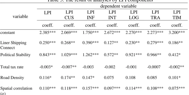
Table 3 presents the result of spatial regression model where the spatial weighted matrix was constructed based on total trading value.
Table 3. The result of analyses by LPI components
variable dependent variable LPI LPI CUS LPI INF LPI INT LPI LOG LPI TRA LPI TIM coeff. coeff. coeff. coeff. coeff. coeff. coeff.
constant 2.385*** 2.069*** 1.750*** 2.672*** 2.270*** 2.273*** 3.200*** Liner Shipping
Connect
0.250*** 0.268** 0.390*** 0.127** 0.230** 0.279*** 0.186** Political Stability 0.843*** 1.029*** 1.262*** 0.572** 0.921*** 0.966** 0.412* Total tax rate -0.003* -0.007** -0.003 -0.002 -0.001 -0.0007 -0.002** Road Density 0.116* 0.174** 0.147* 0.075 0.108 0.085 0.101* Spatial correlation
()
0.110*** 0.118*** 0.157*** 0.097*** 0.114*** 0.108*** 0.075*** CUS: custom, INF: infrastructure, INT: international shipment, LOG: logistics competence, TRA: tracking and tracing, TIM: timeliness
*) significant at =10%, **) significant at =5%, ***) significant at =1%
Table 3 shows that the spatial correlation exists and significant. The spatial correlation for the model with LPI as the dependent variable is 0.110 meaning that the LPI of a country is affected 0.110 point by the neighbor country’s LPI. For the independent variable values, such as the liner shipping connectivity, political stability, total tax rate, and road density, those independent variables influence the LPI score of a country 0.250, 0.843, -0.003, and 0.116 respectively. Several variables have been included into model but those variables causing the spatial correlation not significant (see appendix 6). Furthermore, the table 3 also presents the result of spatial correlation where the other six LPI components were used as dependent variable. The spatial regression model with LPI infrastructure as dependent variable has the highest spatial correlation value, while the lowest is LPI timeliness.
4.2 Analyses by Different Commodity
This analysis was conducted by changing the basis in constructing the spatial weighted matrix. In addition to total trading value, other commodities are selected as the basis in constructing the spatial weighted matrix. The commodities which have been selected are electronics, automotive, and agriculture, forestry and fishing.
The electronic comodity was chosen as a basis of constructing the spatial weighted matrix since this commodity have complex nature of supply chain. Electronic Industry Citizenship Coalition (EEIC) in their report stated that the supply chain for any given electronics product can include hundreds of companies. This is primarily due to the complex nature of electronic products. Unlike a garment (e.g. shirt), an average laptop computer consists of hundreds of individual parts that must be sourced and assembled according to precise specifications. These parts come from all over the world. It means that the electronic commodity is highly depend on global supply chain. For this reason, the electronic commodity is choosen.
The automotive commodity was chosen as a basis in constructing the spatial weighted matrix because this commodity have similar properties with electronic commodity. Automotive product consist of hundreds parts (components) for which most of them must be sourced from outside supplier. Like electronics commodity, these supplier come all over the world and highly depend on global supply chain.
The agriculture, forestry and fishing commodities were chosen in sector analysis because these commodities were used by some manufacturers as a raw materials of their product, but on the other hand most of countries can fulfill their need for these commodities by themself. It is based on this reason that these commodities are assumed to have low dependencies on global supply chain.
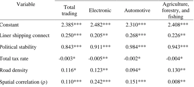
Table 4. presents the comparison of spatial regression analysis result with LPI overall as the dependent variable. There are 4 models shown in table 4, where every model use different basis in constructing spatial weighted matrix.
Table 4. The result of analyses by different commodity
Variable
Basis in constructing spatial weighted matrix
Total
trading Electronic Automotive
Agriculture, forestry, and
fishing Constant 2.385*** 2.482*** 2.310*** 2.408***
Liner shipping connect 0.250*** 0.205** 0.268*** 0.226**
Political stability 0.843*** 0.911*** 0.984*** 0.943***
Total tax rate -0.003* -0.005** -0.002* -0.004*
Road density 0.116* 0.123** 0.094* 0.130**
Spatial correlation () 0.110*** 0.242*** 0.151*** 0.008**
*) significant at =10%, **) significant at =5%, ***) significant at =1%
Table 4 shows the model where the spatial weighted matrix was constructed based on electronic trading value has the spatial correlation () 0.242 which means that in term of electronic trading value the LPI of a country is affected 0.242 point by the neighbor country’s LPI. The independent variables value for liner shipping connectivity, political stability, total tax rate, road density are 0.250, 0.843, -0.003, and 0.116 respectively.
The model where the spatial weighted matrix was constructed based on automotive trading value has the spatial correlation () value 0.151. It means that in term of automotive trading value the LPI of a country affected 0.151 point by neighbor country’s LPI. The independent variables value for liner shipping connectivity, political stability, total tax rate, road density are 0.205, 0.911, -0.005, and 0.123 respectively.
Meanwhile, the model which is the spatial weighted matrix was constructed based on agriculture, forestry, and fishing trading value has the spatial correlation () value 0.008, which means that in term of agriculture, forestry, and fishing trading value the LPI of a country affected 0.008 point by neighbor country’s LPI. The independent variables value for liner shipping connectivity, political stability, total tax rate, road density are 0.226, 0.943, -0.004, and 0.130 respectively.
Table 4. also shows that the spatial regresssion model where the spatial weighted matrix was constructed based on electronic trading value has the highest spatial
correlation () and the model where the spatial weighted matrix constructed based on
agriculture, forestry, and fishing trading value has lowest spatial correlation (). It means that electronics commodity is highly depend on global supply chain. Meanwhile, the agriculture, forestry, and fishing commodity have low dependency on global supply chain, this may be due to most of the countries been able to fulfill their own needs in term of agriculture, forestry, and fishing.
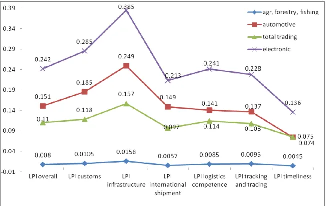
4.3 The Overall Spatial Correlation
Figure 2. shows the comparison of the spatial correlation value () among three commodities in the analyses by different commodity.
Figure 4. The comparison of spatial correlation value of sector analysis.
Figure 2 shows that electronics commodity has the highest spatial correlation followed by automotive commodity, then comes the total trading value, and agriculture, forestry and fishing commodity as the lowest. This indicates that electronics commodity have the highest dependency on international trading (global supply chain) than the other two commodities which were analyzed in the section 4.2.
For the electronic commodity, the spatial correlation for LPI is 0.242, meaning that in term of electronics trading, the LPI of a country is affected 0.242 point by the neighbor country’s LPI. Meanwhile, for the other six LPI dimensions, the highest spatial correlation is LPI infrastucture and the lowest spatial correlation is LPI timeliness. The
automotive commodity has the LPI spatial correlation value 0.127 which means that in term of automotive trading, the LPI of a country is affected 0.151 point by the neighbor country’s LPI. The agriculture, forestry and fishing commodities have the LPI spatial correlation value 0.008. it means that in term of agriculture, forestry and fishing trading, the LPI of a country is affected 0.008 point by the neighbor country’s LPI.
Based on the spatial regression result that electronic commodity has the highest dependency on global supply chain followed by automotive commodity, the Indonesian government should make a policy to improve the electronics and automotive industry by strenghten either the large scale industry and the small and medium industries. Indonesia have a lot of potential electronic and automotive companies which could become a supplier for world class electronic and automotive companies. Indonesian electronic and automotive industries have to participate in global supply chain, because by participating in global supply chain, Indonesia not only become a market for but also become a player in global supply chain. The Indonesian government should enhance the research facility for electronic and automotive industries so that their product able to compete in a global market. Moreover, government should giving the easiness for export import procedure. Furthermore, in regard to the factors that influencing logistics performance in this research, the Indonesian government have to improve the road and shipping infrastructure and also maintain political stability, because political stability will affect to the security and the business is needs stability for business continuity.
5. CONCLUSION
It was found that logistics performance of country’s trading partners affecting to the country’s logistics. This is proven with statistically significant positive spatial correlation values. This research also reveals that logistics performance of a country is affected by its infrastructure such as liner shipping connectivity and road density. Political stability and total tax rate also affecting to the logistics performance. The findings has also shown that the international trade of electronics commodity have high and significant effect on the country’s logistics performance. It can be seen from the analysis where the spatial weighted matrix is constructed based on electronics trading value has higher LPI spatial correlation than the another models where the spatial weighted matrix is constructed based on total trading value, automotive trading value, and agricultural, forestry and fishing trading value.
Further studies should be conducted with considering other factors, such as social factor. The spatial panel model is suggested to be applied in future research to analyze the spatial effect on logistics performance.
REFERENCES
Adhikari, S. “Application of Spatial Regression Analysis for Improved Predictability of Urban Intersection Vehicle Crashes”, Unpublished Dissertation, Illinois Institute of Technology, USA, 2006.
Anderson, J. E. and Wincoop, E., “Trade Cost”, Journal of Economic Literature, Vol. 42, No. 3, pp. 691-751, 2004.
Anselin, L., Spatial Econometrics: Methods and Models, Kluwer Academic, Dordrecht, 1980.
_______________
,Spatial Econometrics, Bruton Center, School of Social Sciences, University of Texas, USA, 2001.
Arvis, et al., Connecting to Compete, Trade Logistics in the Global Economy: The Logistics Performance Index and its Indicators, World Bank, 2007.
_____________
, Connecting to Compete, Trade Logistics in the Global Economy: The Logistics Performance Index and its Indicators, World Bank, 2010.
_____________
, Connecting to Compete, Trade Logistics in the Global Economy: The Logistics Performance Index and its Indicators, World Bank, 2012.
Aten, B., “Does Space Matter? International Comparisons of the Prices of Tradables and Nontradables”, Journal of International Regional Science, vol. 20, pp. 35-52, 1997. Bao, S., Literature Review of Spatial Statistics and Models. Mathsoft, Inc., Seattle, WA, 1990.
Case, A., Rosen, H., and Hines, J., “Budget Spillovers and Fiscal Policy Interdependence: Evidence from the State”, Journal of Public Economy, Vol. 52, pp. 287-307, 1993
Cahill, M., and Mulligan, G. “Spatial Regression Analysis to Explore Local Crime Patterns”, Social Science Computer Review, Vol. 25, No. 2, pp. 174-193. 2007.
Dall'erba, S., “Distribution of Regional Income and Regional Funds in Europe 1989-1999: An Exploratory Spatial Data Analysis”, Annals of Regional Science, Vol. 39, pp. 121-148, (2005).
Doreian, P. Linear Model with Spatially Distributed Data, Spatial Disturbances, or Spatial Effect, Social Method Research, Vol. 9, pp. 29-60, 1980.
Franchois, J. and Manchin, M., “Institutions, Infrastructure, and Trade”, World Development Vol. 46, pp. 165–175, 2013.
Freisthler, B. “A Spatial Analysis Of Social Disorganization, Alcohol Access, and Rates Of Child Maltreatment In Neighborhoods” Children and Youth Services Review, Vol. 26, No. 9, pp 803-819, 2004.
Goh, M. and Ang, A., “Some Logistics Realities in Indochina”, International Journal of Physical Distribution & Logistics Management, Vol. 30, No. 10, pp. 887 – 911, 2000.
Goh, M. and Ling, C., “Logistics development in China”, International Journal of Physical Distribution & Logistics Management, Vol. 33, No. 10, pp. 886-917, 2003.
Gunner, Coskun, and Erman. “Comparison Of Impacts Of Economic And Social Factors On Countries’ Logistics Performances: A Study With 26 OECD Countries”, Research in Logistics & Production Research Paper, ISSN 2083-4950, 2012.
Hausman, W. H., Lee, H. L., and Subramanian, U., “Global Logistics Indicators, Supply Chain Metrics, and Bilateral Trade Patterns”, World Bank Policy Research Working Paper, No.3773, 2005.
_______________
, “The Impact of Logistics Performance on Trade”, Production and Operation Managemennt Journal, Vol. 22, No. 2, , pp. 236–252, ISSN 1059-1478, 2010.
Higazi, et. al., “Application of Spatial Regression Models to Income Poverty Ratios in Middle Delta Contiguous Counties in Egypt”, Master Thesis, Tanta University, Tanta, Egypt, 2013.
Hoeknes and Nicita, “Trade Policy, Trade Cost, and Developing Country Trade”, World Development Journal, Vol. 39, No. 12, pp. 2069-2079, 2011.
Hollweg et al., “Measuring Regulatory Restrictions in Logistics Services”, Journal of Economics and Logistics, Vol. 17, No. 3, pp. 321-338, 2009.
Isik et. al., “Analyzing Regional Fertility Differences in Turkey”, European Journal of Population, Vol. 22, No. 4, pp. 399-421, 2006.
Kam et al., “Spatial Patterns of Rural Poverty and Their Relationship with Welfare Influencing Factors in Bangladesh”. Food Policy, Vol. 30, No. 5, pp. 551-567, 2005. Lehner, M., “Modelling Housing Prices in Singapore using Spatial Regression Analysis”, Master Thesis, Institute for Transport Planning and System, ETH Zurich, Switzerland, 2011.
LeSage, J., Introduction to Spatial Econometrics, Chapman and Hall, Boca Raton, Florida, USA, 1998.
Limao, N. and Venables, A., “Infrastructure, Geographical Disadvantage, Transport Costs, and Trade”, The World Economic Journal, Vol.15, No.3, pp. 451-479, 2001.
Murdoch, J., Sandler, T., and Sargent, K., “A tale of Two Collectives : Sulphur versus Nitrogen Oxides Emission Reduction in Europe”, Journal of Economica, Vol. 64, pp. 281-301, 1997.
Mustra, M. A., “Logistics Performance Index, Connecting to Compete 2010”, UNESCAP Regional Forum and Chief Executives Meeting, New York, 2011.
Navickas, V. and Sujeta, L., “Logistics Systems as a Factor of Country’s Competitiveness”, Journal of Economics and Management, Vol. 25, No.16, pp. 231-237, 2011.
Pinkse, J. and Slade, M., “Contracting in Space: An Application of Spatial Statistics to Discrete Choice Models”, Journal of Econometrics, Vol. 85, pp. 125-154, 1998.
Puertas et al., (2013), Logistics performance and export competitiveness:European experience, Springer Science Business Media, New York, 2013.
Smirnov, O. and Anselin, L., “Fast Maximum Likelihood Estimation of Large Spatial Autoregressive Model : A Characteristics Polynomial Approach”, Journal of Computer and Statistics, Vol. 35, pp. 301-319, 2001.
Subramanian, U. and Arnold. J. Forging Subregional Links in Transport and Trade Facilitation, The World Bank, Washington, DC., 2001.
Subramanian, U. and Lee, Measuring the Impact of the Investment Climate on Total Factor Productivity : Cases of China and Brazil, The World Bank, Washington, DC, 2005. Waller et al., “Quantifying Geographic Variations in Associations between Alcohol Distribution and Violence”, Stochastic Environmental Research and Risk Assessment, Vol. 21, No. 5, pp. 173-188, 2007.
Weng et al., “Analyzing Spatial Variations in Heart Disease Mortality”, Unpublished Dissertation, Kansas State University, 2007.
Wijaya et. al., “Analyzing the Factors that Affecting to TBC Occurence in Bogor”, Master Thesis, Bogor Institute of Agriculture, 2012.
Wilson, J. and Otsuki T., Assessing the Potential Benefit of Trade Facilitation : A Global Perspective. The World Bank, Washington, D.C, 2004.
Yang. Y., “Spatial Effect in Regional Tourism Growth in China”, Journal of Regional Science, Vol. 46, No. 13, pp. 144-162, 2013.
Yu, D. L.,“Spatially Varying Development Mechanisms in the Greater Beijing Area”, Journal of Regional Science, Vol. 1, No. 4,pp. 173-190, 2004.
APPENDIX
Appendix 1 : Indicators in the Logistics Performance Index Survey
The questions in the Logistics Performance Survey delved into the quality of infrastructure, the competence of private and public logistics service providers, the roles of customs and other border agencies, such governance issues as corruption and transparency, and the reliability of the trading system and supply chains. Reliability (measured by the predictability of the clearance process and the timely delivery of shipments) emerged as a key concern, with the difference in satisfaction between the high-and low-performing countries much larger than for any other question in the survey.
Quality of infrastructure
Telecommunications and information technology (IT) infrastructure are an essential component of modern trade processes. The physical movement of goods now entails the efficient and timely exchange of information. In countries in the LPI’s top two quintiles, logistics operators rarely have any issues with the quality of the telecommunications and IT infrastructure, but close to half of them express concerns in countries ranging from average to lowest performers.
The quality of transport infrastructure remains a concern in close to or more than half of the logistics operators in average, low, and lowest performers. That concerns also exist in even the highest and high per-forming countries reflects the challenge of maintaining physical infrastructure at a level able to satisfy rapidly growing demands.
Competence of private and public logistics service providers
The performance of the supply chain depends on the quality of services delivered by the private sector through customs brokers and road transport operators and on the competence and diligence of public agencies in charge of border procedures. In these areas, the three bottom quintiles generally fare much worse than the top quintile, and the differences in quality are as significant as those for infrastructure. For example, the satisfaction with customs brokers is fairly high for the upper-middle-income countries (around 50 percent), but it is only 8 percent for private providers in sub-Saharan Africa.
For the lower performers, the dissatisfaction with the quality of trade logistics services applies to both the private and public sectors. In those countries where logistics performance is high, there is more satisfaction with private providers than with public providers. The negative view of private providers in the lower performers is an important insight. Too often in developing countries, and notably in Africa, inadequate regulations and the absence of competition lead to corruption or poor services such as those provided by “suitcase businessmen” at border posts. Often the mere presence of these operators disturbs the clearance process and hinders the emergence of competent local logistics operators who can work with international operators.
Customs and other border agencies
Clearance at the border is not only a matter of customs diligence. Law enforcement agencies and ministries of agriculture and industry also intervene in the process. Customs performance tends to be better than that of other border agencies; on average, customs clearance accounts for a third of import time. This underscores the importance of addressing the coordination of border agencies, especially in countries that already have attained good customs clearance.
Corruption and transparency
Logistics performance also depends on broader policy dimensions, including the overall business environment, the quality of regulation for logistics services, and, most important, overall governance. The way the local market for logistics services is regulated directly affects a country’s ability to use the physical internet to connect to global markets. The transparency of government procurement, the security of property from theft and looting, macroeconomic conditions, and the underlying strength of institutions are critical factors in determining logistics performance. Unsurprisingly, ratings of the domestic environment in such areas as corruption and the transparency of processes and regulation reflect these findings. The rating for transparency of border processes consistently declines along with LPI scores for the following groups of countries: poor performers in the LPI were also poor performers on transparency of border processes. Solicitation of informal payments is rare among the top 30 countries but common among lower performers.
Reliability of the trading system and supply chains
For traders at the origin or the destination of the supply chain, what matters most is the quality and reliability of logistics services, measured by the predictability of the clearance process and timely delivery of shipments to destination. The difference in satisfaction between the high-and low-performing countries on this question is much larger than for any other question in the survey. Performance data derived from the survey on the time (in days) for delivery of goods confirms the same phenomenon.
Taken together, all these factors quality of infra-structure, the competence of private and public logistics service providers, the roles of customs and other border agencies, governance issues such as corruption and transparency, and the reliability of the trading system and supply chains confirm once again that logistics performance is about predictability. Predictability is central to the overall costs that companies incur in logistics and thus to their competitiveness in global supply chains.
Appendix 2 : The Moran index
The moran index is used as consideration in the selection of those three methods. In the spatial analysis moran index used as a tool that was first used to investigate whether there is spatial effect in the data. Moreover, in this case the moran index can be used to see how well these three methods in mapping the Indonesia’s trading partner countries.
The mapping performance comparison of three rank method Rank method based Moran index Trading value 0.050 Inverse trading 0.122 Inverse proportion of trading value 0.321
Figure : The moran index comparison among three rank methods
The table and figure above show that the ranking method based on inverse proportion of trading value has the highest moran index. This also indicate that this method is better in mapping the Indonesia’s trading partner countries. Thus, the ranking method based on inverse proportion of trading value is chosen as a method in defining countries coordinates.
Appendix 3 : Countries included in the analysis
Australia, Belgium, Brazil, Bulgaria, Canada, Chile, China, Czech Republic, Denmark, Finland, France, Germany, Greece, Hong Kong, India, Indonesia, Italy, Japan, Korea, Latvia, Malaysia, Mexico, Netherland, New Zealand, Norway, Philippines, Poland, Portugal, Romania, Russian, Saudi Arabia, Singapore, Slovenia, South Africa, Spain, Sweden, Switzerland, Thailand, Turkey, United Kingdom, United States, Vietnam.
Appendix 4 : The countries coordinates
The table below presents the countries coordinates based on inverse proportion of trading value. The export data was used as x-axis coordinate and the import data used as y-axis coordinate. Indonesia, used as a reference country, is given coordinate of (0,0). Then calculate either the inverse of export and import proportion for other 41 countries to get the countries coordinates.
The countries coordinates
country coordinate country coordinate country coordinate
x y x y x y
Australia 29.01 32.60 India 39.9 15.1 Romania 1032.5 1051.5
Belgium 228.08 123.56 Indonesia 0.0 0.0 Russian 77.9 201.3
Brazil 81.53 107.58 Italy 104.9 69.3 Saudi Arabia 30.0 98.7
Bulgaria 950.67 973.53 Japan 7.4 5.2 Singapore 6.6 9.7
Canada 79.12 198.54 Korea 15.6 13.6 Slovenia 1078.8 1032.1
Chile 642.64 622.67 Latvia 1357.4 1176.4 South Africa 253.3 121.1
China 6.19 8.40 Malaysia 14.0 16.7 Spain 242.4 69.3
Czech 643.32 717.06 Mexico 338.6 241.2 Sweden 115.7 905.6
Denmark 444.36 525.83 Netherlands 163.4 41.1 Switzerland 253.5 406.5
Finland 319.10 936.42 New Zealand 213.0 353.2 Thailand 15.7 27.0
France 67.87 117.14 Norway 607.8 1976.0 Turkey 316.8 117.1
Germany 37.17 46.37 Philippines 205.1 50.7 UK 113.8 82.6
Greece 794.06 760.21 Poland 787.2 441.8 USA 13.3 10.3
Hong Kong 94.17 60.18 Portugal 1105.0 1109.7 Viet Nam 73.7 77.4
Note: x : inverse of Indonesia’s export proportion to that country y : inverse of Indonesia’s import proportion from that country
Appendix 5 : The statistics summary of variables included in the model
Variable Minimum Maximum Mean Standard Deviation LPI 2.370 4.190 3.502 0.421 LPI Customs 1.940 4.208 3.274 0.517 LPI Infrastructure 2.230 4.336 3.459 0.574 LPI International shipments 2.479 4.049 3.349 0.329 LPI Logistics competence 2.457 4.316 3.486 0.461
LPI Tracking 2.174 4.273 3.562 0.433
LPI Timeliness 2.943 4.529 3.895 0.372 Liner shipping connectivity 0.684 2.194 1.536 0.356 Road density 0.751 2.703 1.723 0.516 Quality of port 2.600 6.831 4.850 1.162 quality of road 2.059 6.663 4.725 1.378 Time to Export 6.000 25.000 13.119 5.160 Total tax rate 14.500 81.200 42.886 13.666
Political Stability 0.405 0.920 0.711 0.094
Appendix 6 : The predictors that have no spatial correlation to LPI
The independent variable which does not have spatial correlation to LPI Variable Cofficient (p.value) Cofficient (p.value) Cofficient (p.value) Cofficient (p.value) Constant 3.426 (0.000) 4.244 (0.000) 2.079 (0.000) 2.079 (0.000) Time to export -0.059 (0.000) Quality of port 0.288 (0.000) Quality of road 0.224 (0.000) Spatial correlation () 0.1076 (0.000) 0.0577 (0.092) 0.0332 (0.06) 0.030 (0.138)
The table above shows that when the spatial regression model did not include any independent variable in the model, the spatial coefficient is 0.1076, and it value is significant with p.value 0.000. The time to export, quality of port, and quality of road variable evidently make the spatial correlation decrease and become not significant. When the time to export variable included to the model, the spatial correlation is 0.0577 with the p.value 0.092 (not significant). Similarly for for both the quality of port and quality of road variable, the spatial correlation value drops to 0.0332 and 0,030 respectively. As for this results, those three variables will not be included into the model due to the fact that those variables make the spatial correlation of LPI become not significant.
Appendix 7 : The result of spatial regression model where spatial weighted matrix constructed based on electronic trading value
variable dependent variable LPI LPI CUS LPI INF LPI INT LPI LOG LPI TRA LPI TIM
coeff. coeff. coeff. coeff. coeff. coeff. coeff.
constant 3.244*** 3.053*** 3.004*** 3.314*** 3.173*** 3.198*** 3.710*** Liner Shipping
Connect
0.085** 0.117** 0.159** 0.027** 0.069** 0.119** 0.050* Political Stability 0.614** 1.033*** 0.626** 0.590** 0.582** 0.381** 0.348** Total tax rate -0.052*** -0.087** -0.068** -0.041** -0.003** -0.032** -0.033** Road Density 0.192*** 0.254*** 0.257*** 0.144** 0.189** 0.164** 0.150** Spatial correlation
()
0.224*** 0.246*** 0.342*** 0.190*** 0.222*** 0.221*** 0.130***
CUS: custom, INF: infrastructure, INT: international shipment, LOG: logistics competence, TRA: tracking and tracing, TIM: timeliness
*) significant at =10%, **) significant at =5%, ***) significant at =1%
Appendix 8 : The result of spatial regression model where spatial weighted matrix constructed based on automotive trading value
variable dependent variable LPI LPI CUS LPI INF LPI INT LPI LOG LPI TRA LPI TIM
coeff. coeff. coeff. coeff. coeff. coeff. coeff.
constant 2.911*** 2.591*** 2.399*** 3.084*** 2.886*** 2.785*** 3.661*** Liner Shipping
Connect
0.1013** 0.115*** 0.219*** 0.018*** 0.080** 0.153*** 0.050* Political Stability 0.385** 0.574*** 0.687** 0.242** 0.334** 0.502** 0.268* Total tax rate -0.003*** -0.007** -0.003*** -0.002*** -0.001*** -0.001*** -0.002*** Road Density 0.162** 0.221** 0.192*** 0.122** 0.163** 0.120** 0.144** Spatial correlation
()
0.127*** 0.160*** 0.224*** 0.121*** 0.213*** 0.218*** 0.113***
CUS: custom, INF: infrastructure, INT: international shipment, LOG: logistics competence, TRA: tracking and tracing, TIM: timeliness
*) significant at =10%, **) significant at =5%, ***) significant at =1%
Appendix 9 : The result of spatial regression model where spatial weighted matrix constructed based on agriculture, forestry, and fishing trading value
variable dependent variable LPI LPI CUS LPI INF LPI INT LPI LOG LPI TRA LPI TIM coeff. coeff. coeff. coeff. coeff. coeff. coeff. constant 2.988*** 2.690*** 2.529*** 3.183*** 2.946*** 2.840*** 3.689*** Liner Shipping Connect 0.054** 0.057** 0.136*** 0.201** 0.039** 0.108** 0.028* Political Stability 0.364*** 0.539*** 0.653*** 0.194** 0.322** 0.501** 0.024* Total tax rate -0.005*** -0.009*** -0.006** -0.003** -0.002** -0.002** -0.003*** Road Density 0.202*** 0.268*** 0.293*** 0.155*** 0.198*** 0.162** 0.164** Spatial
correlation ()
0.0030*** 0.0031*** 0.0035*** 0.0033*** 0.0032*** 0.0031*** 0.002***
CUS: custom, INF: infrastructure, INT: international shipment, LOG: logistics competence, TRA: tracking and tracing, TIM: timeliness
*) significant at =10%, **) significant at =5%, ***) significant at =1%