國 立 交 通 大 學
資 訊 科 學 與 工 程 研 究 所
碩
士
論
文
一個為 Thumb-2 可執行檔
以 LLVM 為基準的靜態二元轉譯系統
An LLVM-based Static Binary Translation System
for the Thumb-2 Executable
研 究 生:劉冠宏
指導教授:徐慰中 教授
一個為 Thumb-2 可執行檔以 LLVM 為基準的靜態二元轉譯系統
An LLVM-based Static Binary Translation System
for the Thumb-2 Executable
研 究 生:劉冠宏 Student:Kuan-Hung Liu
指導教授:徐慰中 博士 Advisor:Wei-Chung Hsu
國 立 交 通 大 學
資 訊 科 學 與 工 程 研 究 所
碩 士 論 文
A ThesisSubmitted to Institute of Computer Science and Engineering College of Computer Science
National Chiao Tung University In partial Fulfillment of the Requirements
for the Degree of Master
In
Computer Science July 2013
Hsinchu, Taiwan, Republic of China
一個為 Thumb-2 可執行檔
以 LLVM 為基準的靜態二元轉譯系統
研究生:劉冠宏
指導教授:徐慰中博士
國 立 交 通 大 學 資 訊 科 學 與 工 程 研 究 所 碩 士 班
摘 要
Thumb-2 是一個 16 位元和 32 位元共存的指令長度可變指令集架構,跟 ARM 架構相 比,他有更高的指令密度,但是效能又很接近 ARM。對靜態二元轉譯系統來說,如何區 分指令和資料,以及找到轉譯前後程式計數器的對應是非常困難的,因此設計一個靜 態二元轉譯系統不是一件簡單的事情。在這篇論文中,我們介紹一個對於 Thumb-2 可 執行檔的靜態二元轉譯系統,它利用了 LLVM 的各項功能去轉譯輸入的檔案、對他做最 佳化、編譯,並且產生輸出的二進位檔。我們的系統利用一些方式找到那些被 GCC 所 產生出來的二進位檔中,被安插在指令間的資料,而且建立了一個轉譯前後程式計數 器的對應表並利用一些方法減少此表的空間。我們亦提供了一些方法改善我們轉譯後 的檔案,使得 LLVM 優化器和編譯器可以更快的完成他們的工作。我們的系統最終產生 x86 架構的可執行檔以便於比較效能,並使用 SPEC2006 CINT 配合具參考價值的輸入資 料來做為比較的依據,就平均的結果來看,我們轉譯後的可執行檔比使用 QEMU 的結果 快了大約 5.6 倍;而跟 x86 原生的可執行檔比較起來,速度大約慢了 2.1 倍,且檔案 大了 2.5 倍。而最後我們提出的一個減少工作時間的方式雖然執行時間多花了三成, 可是轉譯的時間卻快了 13 倍。 iAn LLVM-based Static Binary Translation System
for the Thumb-2 Executable
Student: Kuan-Hung Liu
Advisor: Dr. Wei-Chung Hsu
Degree Program of Computer Science
National Chiao Tung University
ABSTRACT
Thumb-2 is a 16-bit and 32-bit mixed instruction set architecture (ISA), with higher code density compared with ARM, and the performance is close to ARM. The code discovery problem and the code location problem caused by indirect branches make static binary translation (SBT) system hard to develop. In this thesis, we present a SBT system for Thumb-2, which leverage the LLVM infrastructure to translate the source binary into LLVM IR,
optimize and compile the LLVM bitcode file, and then generate the target binary. Our system solves the code discovery problem for the binaries, which are generated by GCC, by finding all kinds of data that are interspersed in the code. The code location problem is also solved by creating an address mapping table with relatively smaller size. We also introduce an approach to reduce the optimization and compilation time of translated LLVM bitcode files. Our system finally generates x86 executable for performance comparison. In our experiments which use SPEC2006 CINT with reference data to be the benchmark, the execution time is about 5.6 times faster than QEMU, while about 2.1 times slower with 2.5 times code expansion when compared with the x86 native binaries. Furthermore, with our saving-time approach, the execution time will be increased by 30% while the translation time could be 13X better.
誌 謝
本論文能夠順利完成,首先必須感謝我的指導教授徐慰中老師,老師帶給我們的 不只是專業領域的知識,還包括許多寶貴的人生經驗和處世態度,都值得讓未來的我 們作為參考,甚至訂為目標;更感謝三位口試委員:吳真貞教授、單智君教授、楊武 教授,不但撥空前來參與我的口試,他們的意見和指教也讓本論文更加的充實和完 整,由衷的感謝他們。也謝謝我的前指導教授莊榮宏老師,願意在我對計算機圖學失 去興趣的時候讓我轉換領域,讓我得以在新的領域貢獻一點微薄的心力。 特別感謝陳俊宇學長和沈柏曄學長在研究上的指導,幫助我突破許多論文上的瓶 頸,讓本論文能夠順利完成;感謝所有 446A 實驗室和計算機圖學與幾何模擬實驗室的 同學、學長姊和學弟妹及助理們,碩士的兩年有你們陪伴,讓我過得很充實也很愉 快,那段一起研究如何泡咖啡的日子,我永遠也不會忘記,真的非常謝謝你們。還要 感謝中華扶輪教育基金會,我得到的不只是金錢上的援助,讓我得以安心念完碩士, 更重要的是,讓我在獎學生聯誼會中,認識一群各領域的菁英,同時也是一群值得信 賴的夥伴,能順利完成論文,他們也功不可沒!此外,每個月的例會更讓我在忙碌的研 究生活中,找到一個喘息的機會,有好多平常沒有機會到訪的地方,都藉由參加例會 一一的實現,由衷的感謝那群支持基金會運作的扶輪社友們以及聯誼會的幹部們。 最後,感謝一直以來支持我、為我操心的家人,讓我一路順利且無後顧之憂的念 完碩士,你們的支持是我最大的力量,也讓我更有勇氣去面對未來的困難。 謝謝所有曾經幫助過我、關心過我的人,在此表達我最誠摯的謝意,有了你們的 支持,未來的我會更加努力。 iiiTable of Contents
摘 要 ... i ABSTRACT ... ii 誌 謝 ... iii Table of Contents ... iv List of Tables ... viList of Figures ... vii
I. Introduction ... 1
II. Background and Related Work ... 4
2.1. Binary translator ... 4
2.1.1. Static Binary Translator ... 4
2.1.2. Dynamic Binary Translator ... 5
2.2. Code Discovery Problem ... 5
2.2.1. Variable-length Instructions ... 5
2.2.2. Register Indirect Jump ... 6
2.2.3. Data Interspersed with the Instructions ... 6
2.2.4. Padding Bytes to align Instructions ... 6
2.3. Code Location Problem... 7
2.4. ARM/Thumb-1 mixed ISA ... 7
2.5. Thumb-2 Instruction Set ... 8
2.6. Low Level Virtual Machine (LLVM) ... 11
2.7. MC2LLVM ... 11
III. Design and Implementation ... 14
3.1. Overview ... 14
3.2. Design Issues ... 17
3.2.1. Code Discovery Problem ... 17
3.2.2. Code Location Problem... 20
3.2.3. Other Problems... 21
3.3. Implementation Detail ... 21
3.3.1. Find All Kinds of Data ... 21
3.3.2. Address Mapping Table ... 25
3.3.3. Register value mapping table ... 29
3.3.4. Partition the main L-function into several L-functions ... 30
3.4. Relaxing the Restrictions ... 37
3.4.1. Using the compiler other than GCC ... 38
3.4.2. Switch Table Analysis ... 38
3.4.3. Case study: ARMCC ... 40
IV. Experimental Results ... 41
4.1. Environment ... 41
4.2. Performance ... 41
4.2.1. Execution Time ... 42
4.2.2. Translation Time ... 52
4.3. Code Size ... 53
V. Conclusion and Future Work ... 55
Reference ... 57
List of Tables
Table 1. Comparison between ARM, Thumb-2 and Thumb ... 10
Table 2. Thumb-2 switch patterns ... 18
Table 3. Statistical information about some of EEMBC benchmarks ... 44
Table 4. The reasons for not runnable benchmarks in CINT2006 ... 45
Table 5. Statistical information about CINT2006 ... 49
Table 6. Comparison between the ratio of Return address and AMT ... 50
List of Figures
Figure 1. Causes of the Code Discovery Problem ... 5
Figure 2. An example of finding Thumb-2 instruction boundaries ... 6
Figure 3. Comparison of 32-bit instruction between ARM and Thumb-2 ... 9
Figure 4. An example of ARM (left) and Thumb-2 (right) binaries ... 9
Figure 5. PC values in three pipeline stages ARM CPU ... 10
Figure 6. An Overview of SBT of mc2llvm ... 12
Figure 7. Memory layout of the target binary ... 13
Figure 8. An overview of our SBT System ... 15
Figure 9. The framework of the translated program. ... 16
Figure 10. An example of padding byte ... 19
Figure 11. An example of set analyzing ... 22
Figure 12. An example of sets union operation ... 22
Figure 13. An example of non-discarding used data version ... 23
Figure 14. An example of discarding used data version ... 23
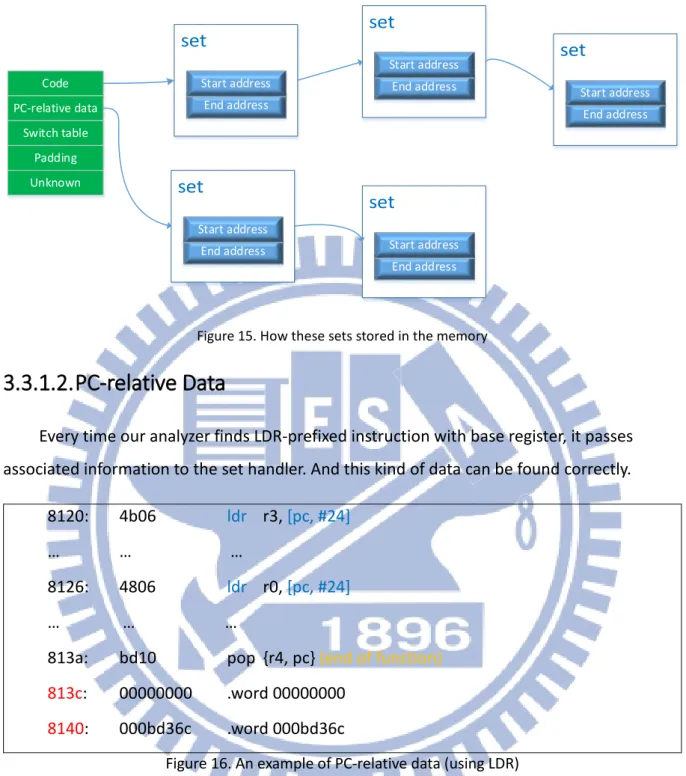
Figure 15. How these sets stored in the memory ... 24
Figure 16. An example of PC-relative data (using LDR) ... 24
Figure 17. Finite State Machine for finding switch cases ... 25
Figure 18. An example of PUSH and POP in finding function entries ... 27
Figure 19. An example of BX in finding function entries ... 27
Figure 20. Diagram of the Address Mapping Table ... 29
Figure 21. A special case of switch case pattern ... 30
Figure 22. An example of how GCC generates LDRD instructions ... 30
Figure 23. Comparison between one function and multi-function ... 31
Figure 24. The framework of multi-function version LLVM module ... 32
Figure 25. An example of function graph ... 33
Figure 26. An example of function switching handler ... 35
Figure 27. The control flow of each slice of LLVM function... 36
Figure 28. An example of mem2reg optimization (STR r0, [SP, #-4]) ... 37
Figure 29. Encoding method of TBB and TBH ... 39
Figure 30. EEMBC execution time... 43
Figure 31. Result of CINT2006 with test data, compared with native result... 46
Figure 32. Result of CINT2006 with ref data, compared with native result ... 47
Figure 33. Result of CINT2006 with test data, compared with our best result ... 48
Figure 34. Result of CINT2006 with ref data, compared with our best result ... 48
Figure 35. Comparison of translation time when handling stripped function ... 49
Figure 36. DFS vs. Uniform... 51
Figure 37. Helper function vs. LLVM switch instruction ... 51
Figure 38. Recursion time comparison: 0 vs. 2048 ... 52
Figure 39. Translation time Ratio ... 53
Figure 40. Code size comparison in CINT2006 ... 54
I.
Introduction
Binary translation [1] techniques have been used in various areas, such as application migration from one ISA (Instruction Set Architecture) to another [2] [3] [4], fast simulations [5], dynamic optimizations [6] [7], and virtual machine implementations [8]. These
techniques have been actively studied and developed in the past decade.
Software-based binary translation can be roughly classified into two categories: SBT (Static Binary Translation) and DBT (Dynamic Binary Translation) [9]. Both of them have pros and cons, but most of production systems and researches are based on DBT. This is because two major problems of SBT, code discovery problem and code discovering problem, can be more effectively and efficiently handled by DBT. DBT has some shortcomings, such as longer start-up time due to initial runtime translation, less aggressive code optimizations for translated binaries compared with SBT, and larger memory footprint due to the use of code cache, the emulation engine and the presence of the dynamic translator. In some
environments, like the embedded systems, that start-up time, power consumption, and memory usage are the primary concerns, using SBT might be more desirable than DBT. Some researcher works offer HBT (hybrid binary translation) [10] that combines the advantages of both SBT and DBT. It uses SBT to translate the guest code as much code as possible statically, and switches to DBT when run-time exceptions occur due to incorrect translation by SBT. Ideally, HBT has the advantage of high performance due to SBT, and the robustness of DBT. However, if the code discovery and code location problems are not effectively solved for SBT, then HBT could fall back to DBT and loses the advantages of SBT. In this thesis, we focus on solving the two problems in SBT for the ARM/Thumb-2 architecture.
ARM [11] [12] architecture is widely used in the mobile computing market and embedded systems. More and more companies adopt ARM processors in their systems, including most smart phones, tablets (including MS Windows RT), and Google Chrome-Book laptops. Recent ARM cortex A15 may start to show up in micro-servers. The original ARM is a RISC (Reduced Instruction Set Computer) ISA, all instructions are fixed-length. However, due to the memory footprint requirements for embedded systems, the ARM architecture has been enhanced with variable length instructions in ARM/Thumb-1 and ARM/Thumb-2.
All instructions in Thumb-1 are 16 bits, and there is a mode bit that indicating the current execution mode is ARM or Thumb-1 for ARM/Thumb-1 mixed mode binaries. To further reduce the code size and increase the performance, Thumb-2 ISA was introduced after ARMv6T2. This thesis concentrates on the translation of Thumb-2 instructions since it achieves performance similar to ARM code, with code density close to Thumb-1. The
difficulty for translation is that Thumb-2 is considered a mixed length (or variable length) ISA which contains both16 bits and 32 bits instructions. With a variable length instruction ISA, code discovery problem becomes an issue. To solve the code discovery problem in the Thumb-2 binary translation, we have to identify all kinds of data embedded in the binary. Data embedded in binary can be PC-relative data, instruction padding and jump/search tables generated from the switch statements. Identify the jump and search tables is challenging, since the code patterns generated from different compilers are not the same. This issue is investigated in this work. In the past, our team developed LLBT [4], and has dealt this problem for ARM and Thumb-1 binaries generated by GCC [13], which is one of the most popular compiler used in the Linux world.
Once the binary is translated to the target-binary, it should be optimized; otherwise, the performance is too poor to be accepted as a desired alternative to DBT. Developing a binary translator that includes decoder, translator, optimizer, assembler, and linker takes too much efforts and these work usually cannot be leveraged when the target is changed, due to the nature of high target-machine-dependence. Therefore, a retargetable binary translator is highly desirable. To implement a retargetable binary translator, the translation pass must be split into target-independent part and target-dependent part, and the interface between the two parts are immediate representation (IR) forms. The front-end of our SBT system
translates the input binary into IR forms and then translates into the binary of target
machine with different ISA by the back-end. Instead of creating a new IR, we lean to leverage an existing compiler infrastructure that can satisfy our requirements to build a
high-performance and retargetable binary translator.
In this thesis, we present a SBT system that leverages the LLVM [14] infrastructure and can translate Thumb-2 ISA to many different target ISAs supported by LLVM. Our work is based on mc2llvm [10], a retargetable hybrid binary translator.
The remainder of the thesis is organized as follows: Chapter II introduces some related work and the techniques used in our work. Chapter III gives the design of our system and describes the implementation details. Chapter IV discusses the experimental results and Chapter V concludes our work and discusses future works.
II. Background and Related Work
In this chapter, we introduce binary translator first, and then describe the main problems we met when constructing a SBT system. Thumb-2 instruction set is also
introduced in this chapter. Previous works on solving the code discovery problem are also included. An overview of the LLVM compiler infrastructure is then described. At the remainder of this chapter, we briefly show how mc2llvm, which is the base of our system, works, and introduce some techniques that are also important for our system.
2.1. Binary translator
Binary translator translates the source binary program into the target binary program whose ISA may be different from the source one. It can be classified into two categories: SBT and DBT, and they translate the source binary off-line and on-line respectively.
2.1.1. Static Binary Translator
Static binary translator translates the source binary into the target binary in static time, so there is no translation overhead when executing translated binary. Besides, more
optimizations can be applied to SBT since the time that costs in compiling time is not that important. Therefore, the performance of the executable generated by SBT is always better than using DBT. However, the programmer must solve the code discovery problem and the code location problem, which are known as the most critical problem when constructing a SBT.
Chen et al. [2] built an SBT that translates the ARM binaries into a MIPS-like platform without using target independent IR. Since all of the ARM instructions are 32-bit instruction, the translator can still work correctly without solving code discovery problem. Their
translator uses an address mapping table to solve code location problem. Furthermore, their translator has a restriction that only the binary generated by GCC can be translated correctly since their translator cannot ensure that it can find all of the indirect branch targets in the binary generated by the compiler other than GCC. This restriction is the same as our system, although our purpose is different.
2.1.2. Dynamic Binary Translator
Dynamic binary translator translates the source binary at run-time, and puts the
translated code in the code cache. An instruction is translated only if the control flow reaches it, so DBT won’t waste any time to translate unused instructions. Therefore, the programmer don’t have to solve the code discovery problem since the control flow never reaches data sections. However, the optimizations that can be applied in DBT is much less than is SBT, because the performance will also be influenced when optimizing.
QEMU [15] is an efficient and retargetable DBT which supports both user-mode and full-system emulations. It is widely used since many popular ISAs are supported and it is an open-source software. QEMU translates the open-source binary instructions into a sequence of micro operations which are implemented by a small pieces of C code. Then these C code will be compiled into the target binary by GCC. Newer version QEMU uses tiny code generator (TCG), which provides a small set of operations, to parse the micro operations and generates the target binaries.
2.2. Code Discovery Problem
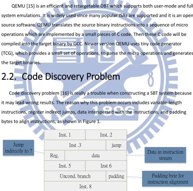
Code discovery problem [16] is really a trouble when constructing a SBT system because it may lead wrong results. The reason why this problem occurs includes variable-length instructions, register indirect jumps, data interspersed with the instructions, and padding bytes to align instructions, as shown in Figure 1.
Inst. 1 Inst. 2
Inst .3 jump
Reg. data
Inst. 5 Inst 6
Uncond. branch padding
Inst. 8 Jump
indirectly to ? Data in instruction
stream
Padding byte for instruction alignment
Figure 1. Causes of the Code Discovery Problem
2.2.1. Variable-length Instructions
If the instructions are fix-length, then all of the instructions can be translated correctly.
Even if data or padding bytes are regarded as an instruction, there is no control flow reaches them. Therefore, misclassification of code and data in the fix-length ISA performs no
influence to the translator, except several dummy instruction blocks may exist in the target binary generated by the translator.
For variable-length instructions, the instruction boundaries may be difficult to find when data interspersed with the instructions. For example, as shown in Figure 2, the instruction that is disassembled from different start address is different. 0x2000 is a MOV instruction but 0x6220 is STR instruction, so the programmer should handle it carefully when designing a SBT.
00 ff
00
20
62 b3 30 31 c0 8b 08 bd 03
Str r0, [r4, #32]
Movs r0, #0
Figure 2. An example of finding Thumb-2 instruction boundaries
2.2.2. Register Indirect Jump
When an indirect jump instruction is encountered, the target address of this jump instruction is held in the register. Determining the content of the register in static time is very difficult, because some of the values are not decidable until run time. Moreover, deciding whether the instruction immediately following the jump instruction is valid is also difficult, since it can be a part of data or padding bytes.
2.2.3. Data Interspersed with the Instructions
Some ISAs allow data interspersed with the instructions, and it makes the SBT more difficult to construct because the data may be regarded as instructions. The kinds of data that may be interspersed with instructions are PC-relative data, switch tables, searching tables … and so on. The manual of ISAs may provide some information about how these kinds of data are usually dealt with. Usually the most difficult reason that the code discovery can’t be solved is because these data can’t be found exactly.
2.2.4. Padding Bytes to align Instructions
Different ISAs have their own alignment restriction. For example, ARM instruction set
must be word-alignment while Thumb-2 instruction set must be halfword-alignment. This kind of bytes may be more difficult to find when using CISC ISAs, like x86. Although some compilers use an NOP (no operation) instruction to implement padding behavior and the programmer can regard them as an instruction, padding bytes with value being certain value is still more common.
2.3. Code Location Problem
Since the source binary is accessed by the source program counter (SPC), while the translated binary is access by the target program counter (TPC), the problem occurs when there is an indirect branch or jump in the source binary. The target address of indirect control transfer is stored in the register and this address is belong to the source binary. The address of the translated binary may be different from the source. Therefore, a SPC address to TPC address mapping is needed; otherwise, the target address for translated binary is still unknown and the result is unpredictable.
2.4. ARM/Thumb-1 mixed ISA
ARM is a 32-bit ISA while Thumb-1 is a 16-bit ISA. Thumb-1 is introduced because many ARM instructions need only 16 bits to encode and it wastes many code spaces. However, the performance of Thumb-1 executable is worse than ARM executable, since more Thumb-1 instructions are needed for performing the same efforts as one ARM instructions. Before Thumb-2 instruction set was introduced, the only way to leverage the pros of these two ISAs is using ARM/Thumb-1 mixed ISA.
ARM/Thumb-1 mixed ISA uses a mode bit to indicate what the current ISA mode is, and the bit 0 of PC to indicate the ISA of branch target region. However, the content of this mode bit is known at run time, and the translator can’t decide which kind of ISA is used for
encoding in the current region, which starts at certain address and ends with a branch instruction, in static time. Fortunately, both of ARM and Thumb-1 are fix-length, so, as we mentioned in 2.2.1, even though the translator regard some data as instructions, it won’t influence the correctness of the translated result. As the result, the code discovery problem in ARM/Thumb-1 ISA is reduced to find which regions should be disassembled as ARM instructions and which should be Thumb-1.
Chen et al [17] introduce a method to distinguish what kind of ISA the current region of instructions were encoded. Their system translates the input binary using ARM and Thumb-1 ISA respectively and gets two version of translated code. Instead of exactly choosing the correct one, their purpose is to discard the regions that must be error-translated. They define “safe region” as the region that is decidable, that is, it must be certain ISA. Safe regions can be found by the entry point of the program from ELF file, head address of each sections, and sections that contain function constructors and destructors. A region of branch targets of safe regions is also a safe region, so many safe regions can be found. Nevertheless, two regions may be linked together by an indirect branch, so there are still a lot of regions that are unknown. Unknown regions can be analyzed and be discarded if some illegal situations occur. They definitely translated an ARM/Thumb-1 executable effectively and correctly, since the code size of translated executable is only about 25% more than the best case and the performance is about 15% slower. This approach may useful when constructing an SBT system for ARM/Thumb-2 mixed ISA.
2.5. Thumb-2 Instruction Set
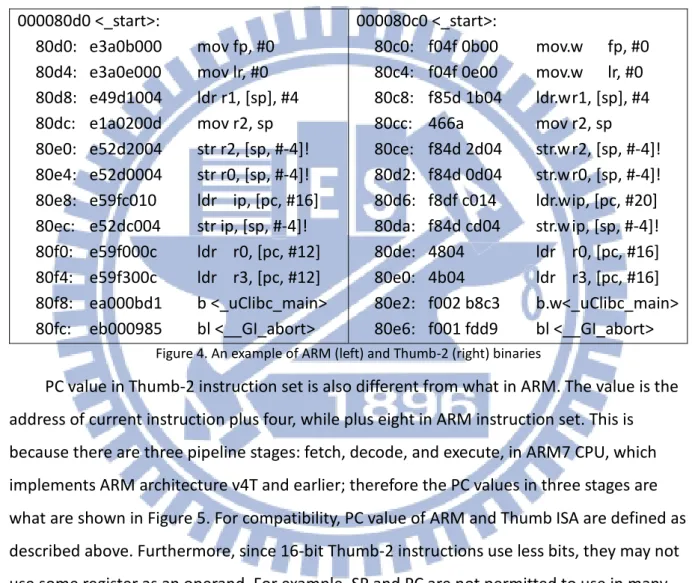
Thumb-2 is a 16-bit and 32-bit mix instruction set with higher code density and almost the same performance compared with ARM instruction set. All of the instructions in Thumb-2 binary are halfword-aligned, so the instruction can start with the address of multiple of two. Furthermore, Thumb-2 instructions are disassembled halfword by halfword, that is, the disassembler reads a halfword at a time, and decide whether it has to read next halfword by the first five bits of this halfword. Only the instructions start with 0b11101, 0b11110 or 0b11111 are regard as 32-bit Thumb-2 instructions. As a result, a continuous four bytes read from the binary are handled in different ways in Thumb-2 instruction set and ARM
instruction set, although they are both 32-bit instructions, as shown in Figure 3. Besides, the instructions that take the same effect are decoded in different ways using these two
instruction sets. Taking Figure 4 as an example, the left column is an ARM binary, and the right one is a Thumb-2 binary. The number of instructions and the efforts of this part of code of two binaries are equal, but the Thumb-2 one uses less space due to 16-bit instructions being used. Obviously, the encoding method of them are also different.
A
A+1
A+2
A+3
A+3
A+2
A+1
A
A+1
A
A+3
A+2
ARM Thumb-2
Figure 3. Comparison of 32-bit instruction between ARM and Thumb-2
000080d0 <_start>: 80d0: e3a0b000 mov fp, #0 80d4: e3a0e000 mov lr, #0 80d8: e49d1004 ldr r1, [sp], #4 80dc: e1a0200d mov r2, sp 80e0: e52d2004 str r2, [sp, #-4]! 80e4: e52d0004 str r0, [sp, #-4]! 80e8: e59fc010 ldr ip, [pc, #16] 80ec: e52dc004 str ip, [sp, #-4]! 80f0: e59f000c ldr r0, [pc, #12] 80f4: e59f300c ldr r3, [pc, #12] 80f8: ea000bd1 b <_uClibc_main> 80fc: eb000985 bl <__GI_abort> 000080c0 <_start>: 80c0: f04f 0b00 mov.w fp, #0 80c4: f04f 0e00 mov.w lr, #0 80c8: f85d 1b04 ldr.w r1, [sp], #4 80cc: 466a mov r2, sp 80ce: f84d 2d04 str.w r2, [sp, #-4]! 80d2: f84d 0d04 str.w r0, [sp, #-4]! 80d6: f8df c014 ldr.w ip, [pc, #20] 80da: f84d cd04 str.w ip, [sp, #-4]! 80de: 4804 ldr r0, [pc, #16] 80e0: 4b04 ldr r3, [pc, #16] 80e2: f002 b8c3 b.w<_uClibc_main> 80e6: f001 fdd9 bl <__GI_abort>
Figure 4. An example of ARM (left) and Thumb-2 (right) binaries
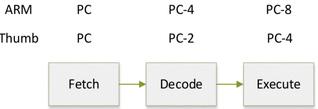
PC value in Thumb-2 instruction set is also different from what in ARM. The value is the address of current instruction plus four, while plus eight in ARM instruction set. This is because there are three pipeline stages: fetch, decode, and execute, in ARM7 CPU, which implements ARM architecture v4T and earlier; therefore the PC values in three stages are what are shown in Figure 5. For compatibility, PC value of ARM and Thumb ISA are defined as described above. Furthermore, since 16-bit Thumb-2 instructions use less bits, they may not use some register as an operand. For example, SP and PC are not permitted to use in many 16-bit instructions. Besides, Thumb-2 instruction set can use IT block, which describe the condition of at most four instructions following the IT instruction, to perform conditional execution if the instructions have no condition code bits. Some comparisons between ARM Thumb-1 and Thumb-2 instruction set are listed in Table 1.
Fetch
Decode
Execute
ARM
Thumb
PC
PC-2
PC-4
PC-8
PC
PC-4
Figure 5. PC values in three pipeline stages ARM CPU Table 1. Comparison between ARM, Thumb-2 and Thumb
ARM Thumb-1 Thumb-2 performance high low close to ARM
Code density low high
Instruction
length 32 bit 16 bit 16 bit and 32 bit Alignment Word-aligned Halfword-aligned
PC Current instruction address plus 8 Current instruction address plus 4
Conditional
execution Condition code IT block and condition code Get 32 bit
instruction A+3, A+2, A+1, A A+1, A+0, A+3, A+2
Code discovery problem in Thumb-2 ISA is not the same as what in ARM/Thumb-1 mixed ISA, although they are both ISAs that contain 16-bit and 32-bit instructions. In ARM/Thumb-1 mixed ISA, the question is how to decide the ISA used for encoding current region, while how to find all kinds of data in Thumb-2 ISA. Moreover, some CPU has ability to run both ARM and Thumb-2 instructions, according to the value of the mode bit, which is the same as what is ARM/Thumb-1 mixed ISA; therefore, ARM/Thumb-2 mixed ISA also exists. To solve the code discovery problem in ARM/Thumb-2 mixed ISA, both deciding ISA of current region and finding data have to be solved, so both the approach in [17] and this thesis may be applied for this purpose.
2.6. Low Level Virtual Machine (LLVM)
LLVM [14] is an open source compiler framework that is developed by University of Illinois. It has ability to convert machine-independent instructions to machine-dependent assembly code. In addition to a static compiler, LLVM also includes Machine Code toolkit [18] which provides several tools for the relating works of the instruction set, such as assembler, disassembler, and object file handler … and so on. Several analysis phases and optimizations have been added to the LLVM infrastructure due to the rapid development in recent years.
LLVM IR is target-independent and must be SSA-form, that is, it can own unlimited virtual registers but each of them can just be defined once. Therefore, optimizations for these IRs can be performed no matter what the target ISA is and the programmer don’t have to argue about the use of the registers.
2.7. MC2LLVM
Our SBT system is based on mc2llvm project, so we will introduce some design details of mc2llvm, especially the parts that also be used in our system.
Mc2llvm is a hybrid binary translator (HBT), which performs the same behavior as SBT in static time, except some routines for calling DBT when exception occurs. An overview of SBT part of mc2llvm is shown in
Figure 6. Since mc2llvm translates ARM binaries to LLVM IR, it don’t need to find the
data interspersed in the code. After translating the binary to LLVM IR, the LLVM optimizer and the LLVM static compiler are used for generating the target assembly code. Finally, the necessary files are linked together and then the target binary is generated.
Once the indirect branch target address cannot be found in the address mapping table, the program will switch to the DBT, which translates instructions from the address one by one until branch instruction occurs and the results are stored in the code cache. Then it switches back to original part of the program that is translated by SBT.
Mc2llvm uses an address mapping table to get the indirect branch target of the binary translated by mc2llvm. The entries in the table are function entries and return addresses, which are more likely to be the branch targets. A hashing function and LLVM switch
instructions are used to construct this table, and the detail will be introduce later since our
system uses similar approach. mc2llvm Target Binary Object reader Source Binary LLVM MC disassembler LLVM
optimizer LLVM static compiler
System assembler System linker Optimized Code Target assembly Object files Source image Linker script Static Translator Section data LLVM IR Runtime System LLVM MC IR Figure 6. An Overview of SBT of mc2llvm
The function initialization routines, including allocating the stack, parsing the command line arguments, setting up the environmental variables, are written in LLVM IR, and this work is the same no matter what source ISA is, so our system uses this module without
unnecessary modification. The system call emulator is implemented by several helper function written in C++ programming language. Since the Linux kernel system calls won’t change if different ISA is used, we apply this emulator in our system, too.
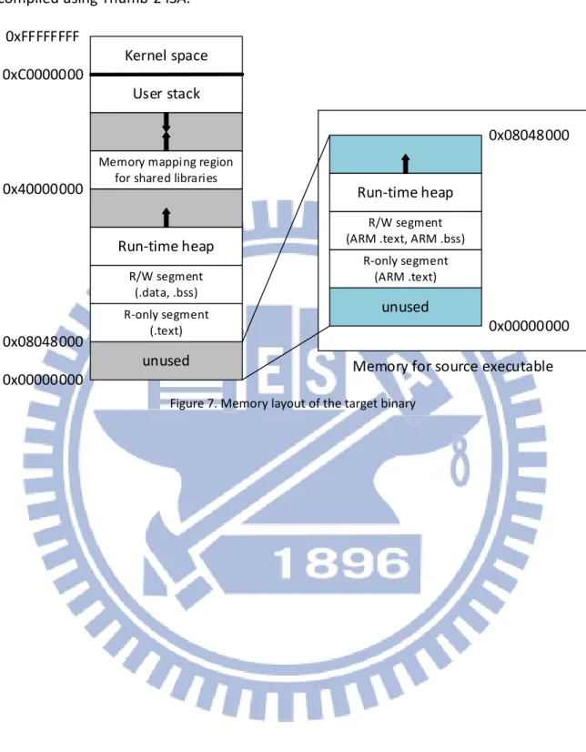
For convenient, mc2llvm maps the memory address of the source binary to the target machine directly; therefore, the output binary uses the memory space beginning with 0x8000 to generate its own memory layout except the stack. As a result, the maximum address of the heap of output binary must be smaller than 0x8048000, which is address of read-only part when loading an binary for Linux system; otherwise, it cause segmentation fault. The memory layout of the target binary is shown in Figure 7. This problem does not exist when the environment is a 64-bit operation system with Linux kernel, since the memory space becomes much larger. This layout is also used in our system, except the source binary
is compiled using Thumb-2 ISA.
User stack
Memory mapping region for shared libraries
Run-time heap R/W segment (.data, .bss) R-only segment (.text) unused R-only segment (ARM .text) R/W segment (ARM .text, ARM .bss)
Run-time heap 0x00000000 0x08048000 0x40000000 0xC0000000 0x00000000 unused 0x08048000
Memory for source executable Kernel space
0xFFFFFFFF
Figure 7. Memory layout of the target binary
III. Design and Implementation
In this chapter, we describe the framework of our static binary translator system first, and then introduce problems, including but not limited to code discovery problem and code location problem, we have to solve and have solved. Moreover, the data structure and methods that are used in our system will also be illustrated. Finally, we introduce some modifications we implemented for certain enhancement. At the remainder of this chapter, we give some discussion about how to relax the restrictions of our program to get a more general SBT.
For convenience, we define “B-function” and “L-function”, which indicate the function from the input executable and the LLVM function generated by our translator, respectively.
3.1. Overview
Our work is based on mc2llvm [10], which is a HBT, so the framework of our SBT system looks like the one in original mc2llvm.
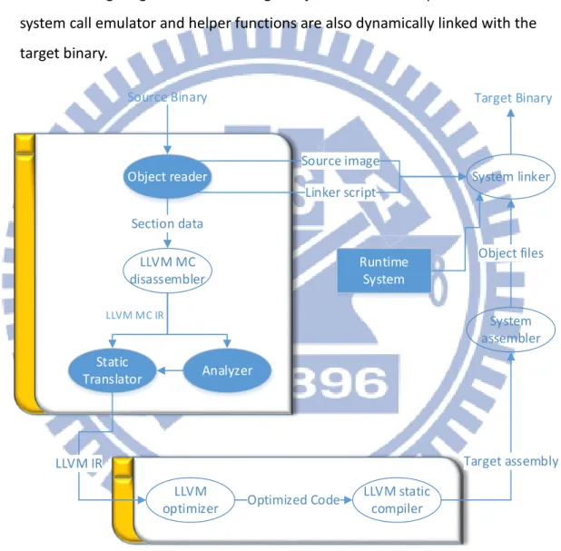
Figure 8 shows the flow of our system. Our system uses LLVM API to read a source binary file, disassemble instructions, and translate them into LLVM IR. Summary of our system is shown as below:
1) Instructions are read by the object reader and decoded by the LLVM MC Disassembler, which is a part of LLVM MC Toolkit. The resource image is also generated in this step.
2) The analyzer analyze the binary and store the information about where is code, where is data, and some statistical data that are useful in the translator.
3) The static binary translator translates the MC IR generated from LLVM MC Disassembler into LLVM IR, and store the results to an LLVM bitcode file.
4) The LLVM optimizer (opt) is used to perform target-independent optimizations on bitcode file generated in 3).
5) The LLVM static compiler (llc) compiles the optimized bitcode file to target assembly, and performs some target-specific optimizations.
6) The target assembler assembles the target assembly and generated target object code.
7) The target linker reads the linker script generated by the object reader and links the resource image together with the target objects. A run-time system that includes a system call emulator and helper functions are also dynamically linked with the target binary. Target Binary Object reader Source Binary LLVM MC disassembler Analyzer LLVM
optimizer LLVM static compiler
System assembler System linker Optimized Code Target assembly Object files Source image Linker script Static Translator Section data LLVM IR Runtime System LLVM MC IR
Figure 8. An overview of our SBT System
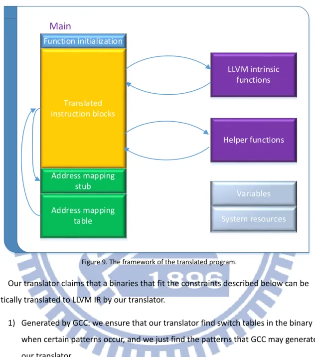
Figure 9 shows how the translated program, which is described by LLVM IR, works. Our translator adds some initialization routine at the beginning of the main LLVM function, including reading command line arguments, initialing the stack …etc. Instructions in the main L-function may call LLVM intrinsic functions or some user-defined helper functions. Every time the indirect branch occurs in the main L-function, the control flow switch to address
mapping stub, which load PC and jump to certain LLVM basic block with corresponding address. The translated program is terminated by some system calls.
Function initialization
Main
Translated instruction blocks Variables LLVM intrinsic functions Address mapping stub Address mapping table Helper functions System resourcesFigure 9. The framework of the translated program.
Our translator claims that a binaries that fit the constraints described below can be statically translated to LLVM IR by our translator.
1) Generated by GCC: we ensure that our translator find switch tables in the binary when certain patterns occur, and we just find the patterns that GCC may generate in our translator.
2) Use static linking: our system is an SBT, so it must be compiled using statically link; otherwise, exceptions occur when calling system libraries or all system libraries should be translated statically.
3) Single thread program: our translator doesn’t support multi-thread and associated system call, so only single thread program can be translated correctly.
4) Use Linux kernel: the system call emulator in our system handles Linux system call
only.
3.2. Design Issues
Code discovery problem and code location problem are the main problem we have to solve. The former is due to we don’t know where is the code and where is the data in the source executable, and the latter is due to the source indirect branch target address is not the same as the target indirect branch target address. For more detail, please see 2.2 and 2.3. We show how we solve these problems and describe other problems we encountered in this chapter.
3.2.1. Code Discovery Problem
As described in 2.5, distinguishing data and code in Thumb-2 binary is the major challenge we have to defeat when solving code discovery problem. Data interspersed with code in the binary make this problem hard to solve, so we classify all of data into several sets first and then conquer each set separately. These data can be classified into four kinds:
1) PC-relative data 2) Switch table 3) Padding
4) Unidentified cases
Once our translator finds all of them, it knows where the data are, and this problem is solved. We will describe how these data generated in Thumb-2 code and how our translator finds them in next section.
3.2.1.1. PC-relative Data
This kind of data are easy to find, since they can be found by load-register instructions, including LDR (unsigned word), LDRB (unsigned byte), LDRSB (signed byte), LDRH (unsigned halfword), LDRSH (signed halfword), LDRD (double word), with PC register being the base. PC register is not permitted to be an operand in all Thumb-2 instructions, and these instructions are examples that are permitted. Notice that PC value must be word-aligned, according to the document of ARM architecture [12].
3.2.1.2. Switch Table
Different compilers may use different patterns to generate switch tables. Since GCC [13] is open source, popular, and widely used in modern world, we can ensure that we can find all switch tables generated by GCC. There are three possible patterns that GCC generates for switch tables, as shown in Table 2. % indicates certain register, and # indicates an immediate value.
Table 2. Thumb-2 switch patterns
– cmp%case, #case_num
– bhi#default_target
tbb [PC, %case] tbh [PC, %case, lsl #1] adr %reg, #table_head ldr PC, [%reg, %case, lsl #2] All Thumb-2 switch tables start with CMP (compare the value) and BHI (branch if greater than). First, the program compares the input value and total number of cases, and then jumps to the default target if the input value is out of range. The third instruction is decided by how many bits are used to indicate one case. TBB (H) uses one (two) bit(s) to indicated one target address, and the remainder uses four bits. The difference of them is what are stored in the table. The offset between target address and current PC is stored when TBB or TBH is chosen, while the target address is stored when the third pattern is used.
The third kind of switch pattern uses ADR instruction before LDR instruction and uses %reg instead of PC, because Thumb-2 has 16-bit and 32-bit instructions and the word data must be word-aligned. There might be a NOP instruction, regarding as a padding instruction, between LDR and the head of switch table if the address of LDR is not word-aligned. Since 16 bit ADR instruction ensure that the address stored in the register must be word-aligned, GCC generates ADR instruction before LDR instruction for fear that NOP influences the head address of switch table.
The offset between switch table and the branch target must be encoded in 9 bits and 17 bits for TBB case and TBH case respectively, and it must be positive (that is, only the
addresses bigger than the table can be branch targets), so the third case is needed since the target address is stored immediately in the data, and all of the addresses in the binary can be
branch targets.
3.2.1.3. Padding
The purpose of using padding data is to make the instructions align word, half-word, or other length of bytes. NOP and NOP.w are frequently used for padding, and they can pad 16-bit and 32-16-bit respectively. Compilers also use 0x0000 as a 16-16-bit padding, and sometimes the padding size may be the multiple of 16 bits for some purpose. Fortunately, 0x0000 is regarded as MOVS r0, r0 when using Thumb-2 ISA; therefore, three cases of padding
described above are all instructions, and they don’t influence any CPU state and control flow of the program, so our translator doesn’t have to regard these cases as special cases.
If other encoding methods of Thumb-2 instructions are also used for padding, they must be decoded and translated without any control flow reaching them. Even though they might consist of some undefined instruction, they can still be handled by regarding them as
unidentified data, described in 3.2.1.4.
Our concern is the padding data that are not regarded as an instruction. This kind of data occurs when GCC generates switch table with TBB instruction and the total number of case is an odd number. Since Thumb-2 must be half-word aligned, a byte data must be padded.
As Figure 10 shows, there are nine cases, numbered from 0 to 8, in this switch table. The address 0xdf32 to 0xdf39 describe the target addresses of case 0 to case 7. Since we assume it is little-endian, the information of case 8 is “0x44”. The next address to be decoded is at df3c, so there must be a padding byte at df3b (0x00 colored orange).
df2a: cmp r3, #8 df2c: bhi.n df3c df2e: tbb [pc, r3] df32: 382c0738--- 4 cases df36: 38311450--- 4 cases df3a: 23000044--- 1 case
Figure 10. An example of padding byte
There might be some strange cases that occurs in hand-writing code for generating padding data due to commercial issues. For example, pad a PC-relative data and some address of word is then marked as a data, so it won’t be translated. In our experiment, PC-relative data are put at the end of functions, because the efficiency of pipeline may be influenced if they are put at the middle of a function; besides, there must be a branch instruction before these data. Therefore, the analyzer can determine whether the data address to load is really a PC-relative data by checking whether the instruction before this address is a branch instruction, or what before this address is also PC-relative data. The remaining case is that it might be the next function entry, and it can be determined by decoding from this data address and checking whether this instruction can be a function entry. The possible characteristic of function entries will be described in 3.3.2.1.
3.2.1.4. Unidentified cases
This kind of data occurs when LLVM disassembler returns fail state. Either these instructions are not supported by LLVM or they use some architectures, like vector float point (VFP), which is not normal architecture of ARM and Thumb-2. This kind of data may also be a kind of padding data. Our translator marks them as a kind of data and don’t translate them for fear that some exceptions occur when executing our translator. The next word-boundary will be the next address for translating, because many Thumb-2 instructions require PC being word-alignment when executing; therefore, less mistranslations occur by handling in this way.
3.2.2. Code Location Problem
Since indirect branch targets can’t be known by our translator in compiling time, a source-PC (SPC) to target-PC (TPC) mapping table is required for translated binaries, and TPC is the head address of an LLVM basic block in our translator. As a result, to make this table usable, our translator must maintain a mapping table from SPC to corresponding basic block.
This table is not difficult to generate, since required information is kept during
translation. The difficulty is how to reduce the size of this table. The larger the table size is, the more time needed for optimizing and compiling; moreover, the execution time is also longer.
3.2.3. Other Problems
Occasionally, the pattern of certain kind of data may have a little difference compared with the normal pattern. For example, an instruction loads a word with the base register that stores the value of PC, and it must be a PC-relative load. Our system must have abilities to find this kind of situations.
Our translator translates all of the source binary into only one LLVM function, named “main”, so LLVM optimizer and LLVM static compiler may take too much time if the source binary is large since optimization unit is a LLVM function. For example, 445.gobmk in
CINT2006, which has about 160 thousand instructions, takes about five hours for translation in our experiment. The complexity of them are at least quadratic, instead of linear, so our translator must have an ability to partition the main function into several smaller L-functions.
3.3. Implementation Detail
In this section, we describe how our translator solves issues described in previous section. A work we implemented may solve more than one issues, so we don’t name the title using the name of issue. The more information our translator gets, the more reliable the translated result is; therefore, we create an analyzer before calling the translator. Our analyzer glances the input binary first to get necessary information and pass them to our translator.
3.3.1. Find All Kinds of Data
3.3.1.1. Data Structure
Although how many memories needed when translating is no concern of our translator, we still want to use a better structure to record these information of the data position.
The most intuitive solution is that use several bits to indicate the data kind of certain half-word. This method is easy to implement, but it cost too much spaces. For example, a binary that contains about one megabytes may need about 200 kilobytes, about one fifth of
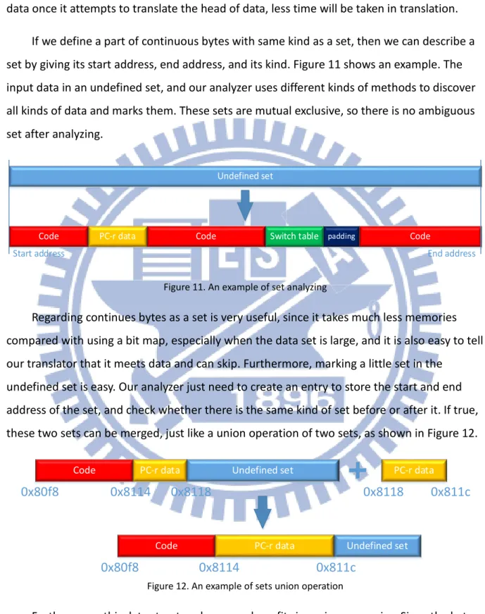
original binary. Besides, our analyzer and translator has to read every halfword one by one even if where it is translating is a large set of data. If our program can jump to the end of data once it attempts to translate the head of data, less time will be taken in translation.
If we define a part of continuous bytes with same kind as a set, then we can describe a set by giving its start address, end address, and its kind. Figure 11 shows an example. The input data in an undefined set, and our analyzer uses different kinds of methods to discover all kinds of data and marks them. These sets are mutual exclusive, so there is no ambiguous set after analyzing.
Undefined set
Code PC-r data Code Switch table padding Code
Start address End address
Figure 11. An example of set analyzing
Regarding continues bytes as a set is very useful, since it takes much less memories compared with using a bit map, especially when the data set is large, and it is also easy to tell our translator that it meets data and can skip. Furthermore, marking a little set in the
undefined set is easy. Our analyzer just need to create an entry to store the start and end address of the set, and check whether there is the same kind of set before or after it. If true, these two sets can be merged, just like a union operation of two sets, as shown in Figure 12.
Code PC-r data Undefined set PC-r data
0x80f8 0x8114 0x8118 0x8118 0x811c
Code PC-r dataPC-r dataPC-r data Undefined set
0x80f8 0x8114 0x811c
Figure 12. An example of sets union operation
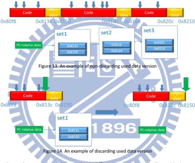
Furthermore, this data structure has more benefits in saving memories. Since the bytes are read sequentially and their address sequence is strictly increasing, our analyzer can discard data whose address is smaller than current halfword. Take Figure 13 and Figure 14 as
an example, Figure 13 shows original version, that our analyzer don’t discard any data that is used, and Figure 14 shows a discarding version. The green arrow indicates that where our analyzer is analyzing and the blue arrows indicate that where are LDR instructions that tell our analyzer where are PC-relative data. As a result, the discarding version uses less memory, since almost all cases of PC-relative data can be merged in only one set. In our experience, only two set entry is needed for the binaries generated by GCC.
0x8150 0x813c PC-relative data 0x81e4 0x81dc 0x8210 0x820c Code dataPC-r 0x80f8 0x813c Code dataPC-r 0x8150 0x81dc Code dataPC-r 0x81e4 0x820c 0x8210
Figure 13. An example of non-discarding used data version
0x8150 0x813c PC-relative data Code dataPC-r 0x80f8 0x813c 0x8150 PC-relative data Code dataPC-r 0x80f8 0x813c 0x8150
Figure 14. An example of discarding used data version
Our analyzer uses linked list to maintain different sets, as shown by Figure 15, since popping the front element and inserting the element at back are needed. Normally, a list of set is in increasing order, so our program just have to check the first set of the certain kind of list and decide what to do. Therefore, our program can execute faster.
End address Start address Code PC-relative data Switch table Padding Unknown End address Start address End address Start address End address Start address End address Start address
Figure 15. How these sets stored in the memory
3.3.1.2. PC-relative Data
Every time our analyzer finds LDR-prefixed instruction with base register, it passes associated information to the set handler. And this kind of data can be found correctly.
8120: 4b06 ldr r3, [pc, #24]
… … …
8126: 4806 ldr r0, [pc, #24]
… … …
813a: bd10 pop {r4, pc} (end of function) 813c: 00000000 .word 00000000
8140: 000bd36c .word 000bd36c
Figure 16. An example of PC-relative data (using LDR)
Take Figure 16 as an example, at 0x8120, the address of the word program has to load is 0x8120 + 4 + 24 = 0x813c, and 0x8120 + 4 is the value of current PC. So our analyzer can mark 0x813c to 0x813f as relative data. Alignment is also important in handling PC-relative data. At 0x8126 in Figure 16, 0x8126 + 4 + 24 = 0x8142 is not the correct target address, because current PC is not word-aligned. The address must be Align(0x8126 + 4, 4) + 24 = 0x8140.
Due to the alignment of PC-relative data, our analyzer can ensure that the instruction at
the address which is not word-aligned is not start point of data, so the probability of mistranslating is lower.
3.3.1.3. Switch Table and Padding
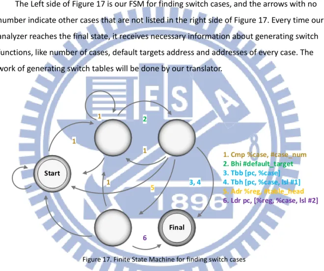
Finite state machine (FSM) is used in our analyzer to find switch tables, because FSM is flexible and easy to implement.
The Left side of Figure 17 is our FSM for finding switch cases, and the arrows with no number indicate other cases that are not listed in the right side of Figure 17. Every time our analyzer reaches the final state, it receives necessary information about generating switch functions, like number of cases, default targets address and addresses of every case. The work of generating switch tables will be done by our translator.
Start Final 2 6 3, 4 1 1 1. Cmp %case, #case_num 2. Bhi #default_target 3. Tbb [pc, %case] 4. Tbh [pc, %case, lsl #1] 5. Adr %reg, #table_head
6. Ldr pc, [%reg, %case, lsl #2]
Figure 17. Finite State Machine for finding switch cases
If the input is TBB when entering the final state, our analyzer have to check whether the number of cases is an odd number, and mark the next byte after the table as a padding byte if true.
3.3.2. Address Mapping Table
Address mapping table (AMT) is created for finding indirect branch targets. The smaller the table is, the shorter the table looking time is. There are only two kinds of possible entries can be indirect branch targets: function entry and return addresses.
3.3.2.1. Function Entry
Function entries can be found in the symbol table, and this is the easiest case.
Unfortunately, sometimes the symbol table is stripped, and our analyzer must have an ability to find the function entries.
There are several possible patterns can be considered as function entries; however, useless entries may also be regarded as function entries, so our analyzer must have ability to handle these entries. Besides, different cases may mark the same address as a function entry, our analyzer don’t discard them since this information can be regarded as a profiling result. Since not all entries found in all cases are real function entries, our analyzer can regard these entries as function entries if it is hit more than certain times. In our experience, the patterns shown below can be a function entry.
1) The address of PUSH instruction with LR included.
2) The address of a 32-bits STMDB instruction with base register being SP and LR is included in operands. The behavior of this STMDB instruction is the same as PUSH instruction.
3) The next instruction immediately follows a POP instruction whose operands include PC.
4) The next instruction immediately follows a 32-bits LDMIA instruction with base register being SP and PC is included in operands. The behavior of this LDMIA instruction is the same as POP instruction.
000a0f2c <__GI_getpid>: a0f2c: b543 push {r0, r1, r6, lr} … a0f3c: bd4c pop {r2, r3, r6, pc} a0f3e: bf00 nop 000a0f40 <__GI_gettimeofday>: a0f40: b557 push {r0, r1, r2, r4, r6, lr} … 26
a0f68: bd5e pop {r1, r2, r3, r4, r6, pc} a0f6a: bf00 nop
Figure 18. An example of PUSH and POP in finding function entries
5) The next instruction immediately follows a BX instruction with operand being LR. 000a59e0 <__pthread_mutex_lock>: a59e0: 2000 movs r0, #0 a59e2: 4770 bx lr 000a59e4 <__pthread_mutex_init>: a59e4: 2000 movs r0, #0 a59e6: 4770 bx lr 000a59e8 <_pthread_cleanup_push_defer>: a59e8: 6001 str r1, [r0, #0] a59ea: 6042 str r2, [r0, #4] a59ec: 4770 bx lr
Figure 19. An example of BX in finding function entries
6) The branch target of BL and BLX instruction. Entries found in this case must be function entries, so our analyzer have to add all of them in the AMT.
7) The address of Function entries may be stored in the PC-relative data. Our analyzer has to check whether the data can be regarded as an entry, and adds it to the AMT if true.
8) The instructions that follow NOP or NOP.W instruction. Since NOP instructions are used for padding and make the address align certain bytes; therefore, this
instruction has higher possibility to be put at the end of the B-function. Sometimes there is a NOP instruction before the function entry because of the
alignment issue, that is, our analyzer may regard the NOP instruction as a function entry in 3), 4) and 5). Our analyzer has to check whether this instruction exists for fear that adding no use entry in the AMT.
All of the B-functions end with branch instructions, no matter indirect or direct. Most of
the cases have been included as described above, but the cases that a B-function end with an unconditional branch instruction is not included.
Conditional branches can’t be the end of B-function because the control flow must reach the next instruction if the condition fails, and instruction address following function call instructions are regarded as the return address, which describes in 3.3.2.2. As a result, only the address of instruction following B or B.W must be recorded. However, putting all of this kind of addresses in the AMT may cause the optimization time and compiler time much longer, even exhausting the memory. Therefore, our analyzer stores all of this kind of
addresses in a secondary address mapping table, and lets the output binary search it if the searching of primary AMT fails. In our system, we maintain this secondary AMT by using LLVM switch instructions, which is the same as the original AMT and described in 3.3.2.3, and LLVM indirect branch instructions, which calls a helper function to search the target before it.
3.3.2.2. Function Return Address
Return address is the address that the function returns to. It is the address of the instruction that is immediately follows the function call instruction, like BL and BLX. Our analyzer stores all of this kind of entries in the AMT.
3.3.2.3. The AMT in LLVM IR
Our translator generate the LLVM switch instruction to handle the AMT, because it knows all of the entries from our analyzer, and using switch instruction is easier to generate direct jump to different entries. Since our analyzer only gets a portion of possible entries from the input binary, the AMT table will be too sparse if we put all of the entries in an LLVM switch instruction. Therefore, the compilers will generate a sequence of if-else instructions for switch instruction instead of a jump table. This will result in a bad performance for searching an address in the AMT. To solve this problem, we use a modulo-function as a hash function to split a large switch statement into several small switch statements.
Figure 20 shows an example of the AMT. The number of tables is dependent on how many possible entries our analyzer found, and it is assumed a power of two because simpler operation can be used when hashing. As a result, even the entry addresses in the level-2 table are still sparse, the number of if-else instructions must be much smaller than the one
without hashing. Table 0 0 Table 1 1 ... Table 31 31 0x740428 0x80c0 0x780407 0x8300 ... ... ... ... Level 1 Table 0 Table 1 Table 31 Table Hash number TPC SPC
Figure 20. Diagram of the Address Mapping Table
3.3.3. Register value mapping table
In some cases, finding PC-relative data and switch tables is not as simple as what described above, due to some limitations of Thumb-2 architecture and different method used by the compiler.
For example, as shown in Figure 21, the address 0x8900 to 0x890b should be marked as a switch pattern by our analyzer, since the value of number of cases is stored in R2 at the address 0x88fa. This is because that the CMP instruction at 0x8900 is a 16-bit instruction, so only eight bits can be used for describing the immediate value. It is obvious that #558 can’t be encoded using only eight bits. Another case is shown in Figure 22, the compiler generates an instruction that store data base, which is dependent on PC, in the register, and the
following is an instruction that loads two words of data start at the base. This ADR instruction is put for alignment issue.
• 88fa: movw r2, #558
• 88fe: subs r3, r0, #1 • 8900: cmp r3, r2 • 8902: bhi.w 9306 • 8906: adr r1, 890c • 8908: ldr.w pc, [r1, r3, lsl #2] • 890C: ...(switch table)...
Figure 21. A special case of switch case pattern
• adr %reg_base, current_pc
• ldrd %reg1, %reg2, [%reg_base]
Figure 22. An example of how GCC generates LDRD instructions
Two cases described above make our analyzer get wrong information that is important for our translator. Therefore, our analyzer should maintain a table that can record the value that is decidable in static time in the register, that is, what our analyzer records is the last value of each registers. Therefore, no matter how many instructions are located between the “get value” instruction and “use value” instruction, our analyzer definitely gets the correct information it needs. Moreover, this table should be flushed when reaching branch
instructions for fear that the analyzer gets wrong information.
Constant folding and constant propagation technology can also be implemented using this table. However, our translator is static and the LLVM optimizer has ability to take these optimization, so we did not implement these optimization here.
3.3.4. Partition the main L-function into several L-functions
The complexity of LLVM optimizer and static compiler are at least polynomial with power greater than one. Since our translator works quickly, the speed of LLVM optimizer and static compiler dominates the execution time of our system. If we can lower the size of the main function, our system can generate translated binary faster.
The comparison between one function method and multi-function method, which distributes instruction blocks uniformly, are shown in Figure 23. Furthermore, the
distribution method can be changed if the user wants. We introduce how our analyzer and
translator partition the main L-function and distribute them into different L-functions. Moreover, we also introduce the method we implemented for handling function switching and some modification for fitting the optimizations of LLVM optimizer.
Original Binary contains n instructions Instruction block 1 Instruction block 2 Instruction block 3 Instruction block 4 …... Instruction block n Containing instruction block 1 to n Instruction block 1 to n/4 Instruction block n/2+1 to 3n/4 Instruction block n/4 + 1 to n/2 Instruction block 3n/4+1 to n Main function
Slice function 1 Slice function 2
Slice function 3 Slice function 4
translate
original
New method
Figure 23. Comparison between one function and multi-function
3.3.4.1. Overview
Figure 24 is the framework of the LLVM module that our system generates using multiple LLVM functions. Since the architecture states and Application Program Status Register (APSR) are regarded as global variables in the LLVM module, we don’t have to pass any of them as parameters when switching L-functions.
In multi-L-function version, the main L-function just handle some initialing routine, like initialing stack space, putting command line arguments and environmental setting in the stack, and then jump to the L-function that contains the instruction block whose address is entry point of the input binary; moreover, since frequently switching between functions may cause stack overflow, we let the slices of L-function return to the main L-function if needed. Therefore, the main L-function must have an ability for handling function switching,
regarding as a switching stub.
Other slices of L-function may call others if branch target is not in it. Besides, indirect branch table is also partitioned in several part, and they are appended to the end of each slice of L-function. Main function initialization Handling function switching Instruction blocks Handling indirect branches
Main Slice function 1
... ... ---Instruction blocks Handling indirect branches Slice function n
Architecture states APSR
Figure 24. The framework of multi-function version LLVM module
3.3.4.2. How many LLVM functions have to be generated
The size of each L-function is user defined and the size of all instructions in the input binary divides by this user defined value; however, we have to avoid that certain L-function becomes too small, so L-function size is permitted to be a little larger than defined if this situation happens.
3.3.4.3. Strategy for distributing instruction blocks
The cost of function switching is not high, but this cost may influence the performance seriously if they switch frequently. Our goal is to lower the frequency of function switching by finding instructions that have more probability to be executed sequentially. Therefore, the instructions in the same B-function must be distributed to the same L-function.
Since the only useful information our analyzer can get is the target address of calling
function, so our analyzer has to find all function entries in the input binary first. How to find the entries of B-function has been described in 3.3.2.1. Then our analyzer constructs a graph, regarding each function as a node and a calling action as an edge. Take Figure 25 as an
example, F1 calls F2 and F3, so there are one direct edge from F1 to F2 and one from F1 to F3.
F1
F2
F3
... ... Bl F2 ... ... Bl F3 ... Bl F3 Bx lr ... Bx lr F1 F3 F2Figure 25. An example of function graph
After generating this graph, our analyzer performs depth first search (DFS) to find all connective components and put the B-function pointer in the list. Each search is start at the node with zero in-edge, that is, no other B-function calls it. However, since the graph is directional, this approach will find two components if two functions which no other B-function calls them calls the same B-B-function. To have more probability that the same component are distributed to the same L-function, our analyzer regards the case described above as only one component.
Finally, our analyzer sorts all components according to their size, and then distributes them, beginning with the largest one. A component will be split into several components if no L-function has enough space to hold it. Besides, some flexible coefficients are added here for fear that some component is just less than 10% larger than the maximal space. This approach may lower the compiling speed, but it is worth since the component won’t be split.
We choose DFS instead of other searching method like breath first search (BFS), because the recording order of B-functions in a connective component is based on which is traced
first. We should ensure that not only the B-functions in the same connective components but also the longest path in the graph has more probability to be distributed into the same L-function.
Our analyzer also implements uniform distribution method. It just distribute B-functions sequentially until the size of L-function larger than user defined threshold. Although the performance of this method is usually worse, it has advantage when handling function switching, as described in the following section.
3.3.4.4. Function mapping table
To find where the instruction block of indirect branch target is, our analyzer has to maintain a table for this purpose. Since indirect branch targets are either function entries or return addresses, we can use the same method used in 3.3.2.3, except that it uses call-instruction instead of branch-call-instruction.
We can also use helper function to find the target LLVM function. Binary search is used in this helper function, and each entry contains address of B-function head, address of next B-function head, and L-function it was distributed. The helper function claim that it finds the target if the target address is between the first two values of the entry. The advantage of this approach is that if the target is not one of the function entries, the translated program can still find the corresponding LLVM function. Although binary search is the best search
algorithm, it still takes time if it searches the same target frequently. Therefore, we also add a function table cache to enhance the performance.
Using helper function is efficient if uniform distribution strategy is used. Since the B-functions that are distributed to the same L-function are put continuously in the input binary, these functions can be described in the same table entry. As a result, the number of entries used in helper function is equal to the number of slices of LLVM functions, and the search time becomes very low.
3.3.4.5. Function switching
The easiest method for L-function switching is just call another L-function directly, but this approach occasions stack overflow if switching behavior occurs frequently. We use two