國 立 交 通 大 學
財 務 金 融 研 究 所
碩 士 論 文
盈餘管理對負債到期結構選擇之影響
The Impact of Earnings Management on the Choice
of Debt Maturity Structure
研 究 生:張詩政
指導教授:林建榮 博士
盈餘管理對負債到期結構選擇之影響
The Impact of Earnings Management on the Choice of Debt
Maturity Structure
研 究 生:張詩政 Student :Shih-Cheng Chang
指導教授: 林建榮 博士 Advisor : Dr. Jane-Raung Lin
國立交通大學
財務金融研究所碩士班
碩士論文
A Thesis
Submitted to Graduate Institute of Finance
National Chiao Tung University
in Partial Fulfillment of the Requirements
for the Degree of
Master of Science
in
Finance
June 2008
Hsinchu, Taiwan, Republic of China
盈餘管理對負債到期結構選擇之影響
研究生:張詩政
指導教授:林建榮 博士
國立交通大學財務金融研究所碩士班
2008 年 6 月
摘要 摘要 摘要 摘要:::: 過去文獻已研究出許多影響公司債券到期日結構決策的因素,分析在不同假說設定下, 對債券到期日長短選擇的影響。本文目的在於研究盈餘管理的行為是否會對負債到期結 構之選擇有所影響,此外,亦討論採取盈餘管理的公司在發行債券後之長期績效。實證 結果發現,發行債券前,公司若採取在財務報表上呈現較高盈餘之盈餘管理(積極盈餘 管理),公司愈有企圖發行到期日較長之債券,持有較高比例長期負債在其資本結構中, 以避免外部頻繁的監控及較高之短期債券重複發行成本。實證亦證實採取積極盈餘管理 的公司在發行債券後的五年內,會有負向的長期績效,顯示當投資人發現公司操縱盈餘 事實時,將對其失去信心,進而反映在公司長期股票報酬的表現上。 關鍵字:負債到期結構;盈餘管理;長期績效The Impact of Earnings Management on the Choice of Debt
Maturity Structure
Student: Shih-Cheng Chang Advisor:
Dr. Jane-Raung Lin
Graduate Institute of Finance
National Chiao Tung University
June 2008
Abstract
Previous analysis has advanced many factors that will affect the firms’ choice of debt maturity structure. The main goal of our study is to examine the relationship between the debt maturity structure and the behavior of earnings management. Besides, we also measure the long-term stock return performance of these firms after issuing debt. From the empirical results, we find that firms which take earnings management to report higher earnings (aggressive) will have incentive to issue debt with longer maturity in order to avoid the frequent outside monitoring and higher issuing cost of short-term debt. In addition, we find that these firms with aggressive earnings management will face 5-year negative long-term stock return performance and indicate that after the manipulation is revealed, investor will lose their confidence and reflect on firms’ stock return performance.
誌 謝
本論文的完成,首先要感謝指導教授林建榮老師,在我論文的寫作上給予許多幫助 與指導,也非常感謝周德瑋老師在我論文程式、資料處理、論文架構上給予許多建議與 想法,讓我能順利完成論文。此外,也要感謝口試委員:陳勝源老師、王祝三老師、李 漢星老師對本論文的意見與指正,提供我更多元的思考方向,也幫助本論文能更臻完整。 研究所兩年以來,很謝謝全所同學的照顧,也謝謝跟我同組的夥伴們,陪我ㄧ起走 過論文寫作這段充滿艱辛的路程。謝謝以文從大學以來對我的照顧、支持,給我許多安 慰和鼓勵,也帶給我許多歡樂;謝謝渝薇,當了ㄧ年的室友,妳開朗的個性總是能讓我 很開心,一起分享彼此的心情;謝謝不常出現在宿舍的文娟,每次出現都會開心的跟大 家聊天,分享趣事。謝謝建佑和文誠,每天大老遠走來陪我們吃飯,有是需要幫忙時, 熱心的伸出援手。謝謝其他所有財金所的同學,謝謝你們這兩年來跟我共同創造的回 憶,我會永遠記在心裡;也謝謝所有財金所的老師,感謝您們諄諄的教誨,幫助我學習 更多的專業知識充實自己。 最後,我要謝謝我父母,總是給我最大的關心與鼓勵,讓我沒有煩惱地順利完成我 的學業,我也要感謝我三個姊姊,從小就是我最好的家庭教師,現在也是提供我未來規 劃很多意見的智囊團,也給我許多幫助。在我人生的旅途中,很高興有我的家人陪伴我, 讓我幸福的成長。謹以此論文,獻給我的家人、師長、同學,以及所有愛我、關心我、 幫助我的朋友,也獻上我誠摯的感謝。 張詩政 謹誌於國立交通大學財務金融研究所碩士班 中華民國九十七年六月於新竹Content
摘要 摘要 摘要 摘要...i Abstract ...ii 1. Introduction ...1 2. Literature Review ...42.1. The theory of debt maturity………..4
2.2. Earnings management………...7
3. Data and Variables... 10
3.1. Data ………..10
3.2. Measurement of Earnings Management ………...10
3.3. Definition of Variables……….11
3.4. Descriptive Statistics………14
4. Methodology... 16
4.1. Ordinary Least Squares Regression………...16
4.2. Two-stage Least Square Regression………...16
4.3. Buy-and-Hold Abnormal Return (BHAR)………17
4.4. Three-factor Model of Fama and French………...18
5. Empirical Results ... 19
5.1. Results of Ordinary Least Square Regression………..19
5.2. Results of Two-stage Least Square Regression………...19
5.3. Results of Long-term Performance of Buy-and-Hold Abnormal Returns (BHAR)………...20
5.4. Results of Long-term Performance of Fama and French Three-factor Model……….21
6. Conclusion ... 23
Listing Table
Table ⅠⅠⅠⅠDistribution of Sample... 26
Table ⅡⅡⅡⅡSummary of Descriptive Statistics ... 28
Table ⅢⅢⅢⅢPearson Correlations ... 30
Table ⅣⅣⅣⅣOrdinary Least Squares Regression Predicting Debt Maturity
Structure………31
Table ⅤⅤⅤⅤTwo-Stage Least Squares Regression Predicting Debt Maturity... 32
Table ⅥⅥⅥⅥLong-Term Stock Returns Performance of Buy-and-Hold
Abnormal Returns………34
Table ⅦⅦⅦⅦLong-Term Stock Returns Performance of Fama and French
1. Introduction
In the past years, many researches have discussed how firms decide their capital structure and debt maturity structure. In recent years, many studies focus on the agency problems. Regarding the agent conflicts between bondholders and stockholders, the interests of bondholders and stockholders may not be consistent. If the interests of both sides could not align, stockholders might give up some of the project with positive NPV and lead to underinvestment. The studies find that the existence of debt can help mitigate the agency problem. If the interests could align, short-term debt can avoid the underinvestment induced by agency problem.
Agency problem also exists between stockholders and managers, whose interests are different. Managers tend to extend debt maturity to avoid outside monitors. However, stockholders hope that there is stricter monitoring that could protect their rights.
However, issuing debt in shorter maturity causes the problem of liquidity risk. Firms issuing short-term debt might have refinance risk, and might bear higher costs of debt refinancing. In contrast, the liquidity risk problem of long-term debt is less serious, but long-term debt could not take the advantage of frequency outside monitoring as issuing short-term debt.
Informational asymmetry exists between managers and potential investors. Managers have more inside information about the firms, so they know the true value of firms more precisely. Earlier literatures present that in order to acquire funds for financing successfully, low-quality firms have the incentive to mimic high-quality firms. The choice of debt maturity would be influenced by the incentive of imitation. However, if the costs of imitation are too high, it is quite difficult for low-quality firms to engage in imitation. In this situation, low-quality firms tend to issue longer maturity debts to avoid facing liquidity risk when their true value is exposed. Nevertheless, it is possible that managers might manipulate earnings
to exaggerate the financial reports of corporations and to mislead outside investors’ evaluation of firms. By doing so, firms might acquire funds for financing more easily.
Gupta and Fields (2006) find that firms with more current liabilities will be affected by earnings management more easily. Our study explores the relationship between debt maturity structure and earnings management. We focus on the problem of asymmetric information between managers and outside investors. Most outside investors use financial reports to evaluate the performance of firms. Investors believe that earnings in the financial reports can reflect firms’ performances. Therefore, managers have incentive to engage in earnings management to decorate financial reports. The behaviors would mislead outside investors and make them too optimistic on firms’ performances. Outside investors would overestimate the true value of firms so as to will affect their decisions of investment. According to signaling theory, firms that engage in earnings management would be likely to issue debt with longer maturity to avoid paying higher costs of debt issues after their real information is exposed. Therefore, this study speculates that managers who engage in earnings management tend to choose to issue debt with longer term to maturity in their capital structure.
This study collects firms that issue debt during 1981-2002 as sample to analyze whether the behaviors of earnings management before the date of debt issues affect the determinants debt maturity. In addition, we also discuss the long-term performance of firms with earnings management after issuing debt. We find that discretionary current accruals are significantly positively related to debt maturity. It indicates that the behavior of earnings management will affect the choice of debt maturity structure. Furthermore, we find that the long-term stock return of firms with aggressive earnings management after issuing debt is poor as our prediction.
we review previous literatures which are related to debt maturity structure and earnings management. In Section 3 we shows the data collection and the definition of all variables that be used in our study and shows the descriptive statistics of our sample. Section 4 provides the methods used for testing our hypothesis. Section 5 presents our empirical results. Finally, Section 6 summarizes our conclusions.
2. Literature Review
In this section, we will review previous literatures about debt maturity structure, and earnings management.
2.1. The theory of debt maturity
A.
Agency cost of debt
Using the concept of options, Myers’ (1977) regards growth opportunity as a call
options of real assets whose exercise price is the capital of future investment, and the exercise value depends on the asset value in the future. As many studies argued, there are interest conflicts between stockholders and bondholders. While firms use risky debt to finance their investment project, the benefits of investment should be split into bondholders and stockholders. The profits of bondholders are fixed; however, the profits of stockholders are uncertain. For this reason, stockholders may choose second-best investment strategies, and firms may lose some investment opportunities with positive NPV or have to burden the costs of the strategies that avoid taking second-best investment projects. Myers’ presents that the problems of underinvestment could be abated by decreasing the maturity of debt. If firms use short-term debt to finance, the lenders and borrowers would recontract before growth options are exercised. Thus, firms with more growth opportunities in their investment projects will have more incentive to issue short-term debt.
According to agency cost hypothesis, Smith (1986) suggests that compare with managers of unregulated firms, managers of regulated firms have less discretion to future investment decisions. Thus, regulated firms would have more long-term debts.
Barclay and Smith (1995) also confirm the respects of Myers’ theory, their research finds that firms with less growth opportunities have more long-term debt in their capital structure. Furthermore, Barclay and Smith argue that firm size is also relative to the maturity structure of debt. The costs of debt public issue have significant economic scale. However, small firms
would hardly take the advantage of economic scale, thus they prefer to choose private debt and more short-term debt which with lower cost of issue. On the other side, the multi-national corporations will choose more short-term debt. If large firms execute board operation, they would like to issue foreign debts. However, the foreign debts have less liquid than bond market in the United States, thus they would prefer to issue short-term debt. Therefore, the positive relationship between firm size and debt maturity of the large firms that execute board operations is decreasing. Smith and Warner (1979) also presents that small firms face more serious conflicts between stockholders and bondholders than large and well-developed firms. Therefore, small firms would like to eliminate the conflicts by issuing short-term debt.
B.
Term structure
Brick and Ravid (1985) use the model including tax to analyze the maturity structure of debt. Because of agency problem, there is optimal term to maturity of debt. However, in the situation of including tax, when the slope of yield curve is positive, (after the adjustment of default risk), it is the optimal decision to issue debt with longer maturity. When the slope of yield curve is negative, the optimal choice is choosing debt with shorter maturity.
Furthermore, if the yield curve is upward, according to expected hypothesis, the interest payment of long-term debt is higher than the expected interest payment of refinancing with short-term debt. However, the interest payment of long-term debt is less than short-term debt in later years. In this condition, issuing long-term debt could reduce the expected tax burden of firms, and increase the short-term value of firms. Therefore, if the term structure is upward, as tax rate increasing, firms would tend to choose more long-term debts.
C. Asymmetric information and liquidity risk
Flannery (1986) suggests that when the information possessed by outside investors is the same with insiders of firms, they would have the same evaluation of firms’ debt. If there are asymmetric information problems in the bond market, the insider would like to issue debt
with overestimated value, the outside investors will misunderstand the true value of firms, and firms whose true value are good will suffer loss. Firms can signal them by choosing the structure of debt maturity. If the transaction cost is low, there is only pooled equilibrium in the market, low-quality firms do not need to pay any cost to imitate high-quality firms, so all of the firms will choose to issue short-term debt. If the transaction cost is high, separated equilibrium might occur, high-quality firms could issue short-term debt to signal their true value to outsiders, and if the cost of imitation was too high, low-quality firms can only issue long-term debt.
Diamond (1991) analyzes the structure of debt maturity with the information of borrowers’ credit rating. The differences of credit rating will also affect the decision of the debt maturity structure. If the insiders have positive information for future development, firms would prefer to issue debt with shorter debt maturity. When debt matures, firms can still refinance by issuing debt successfully, and their problems of liquidity risk are less, and firms could also signal their positive foreground of future by issuing short-term debt. Therefore, Diamond argues that firms with higher credit rating prefer to issue short-term debt. Firms with lower credit rating have no choice but only to issue short-term debt because their profits could not afford for long-term debt. Firms with credit rating between the two extreme sides prefer long-term debt.
Guedes and Opler (1996) support the argument of Diamond. Because the problems of moral hazard exist, low quality firms could not enter into the bond market. Their research finds that firms with investment grade credit rating issue debt with longer maturity or shorter maturity. However, firms with speculative grade credit rating choose to issue debt with medium maturity. In order to avoid liquidity risk and the risk of inefficient payment, firms with higher risk (speculative grade) would not like to issue short-term debt and intend to issue debt with longest maturity that they could issue. However, firms with higher risk would be
obstructed in the long-term debt market because there will be moral hazard problems when requested return leads to risk transference.
Stohs and Mauer (1996) argue that firms with lower leverage would like to have less financial distress and have lower liquidity risk. Thus, those firms have less incentive to manipulate debt maturity. On the other hand, firms with higher leverage will prefer to issue long-term debt.
D. Matching hypothesis
Previous literatures argue that if debt has shorter maturity than assets, firms may be short of cash of repayment. Thus, debt maturity should match with assets maturity. Myers’ (1977) presents that firms will arrange the payment of debt match with the decreasing of assets value, and reduce the agency cost of debt by this way. Therefore, firms with more long-term assets could afford to more long-term debt. The matching of maturity will make firms could extend the maturity of long-term debt in the condition of non-significantly increasing of agency cost of debt.
E.
Managerial stock ownership
Datta, Iskandar-Datta, and Raman (2005) suggest that managerial stockholders play an important role in the decision of the structure of debt maturity. Managers who own the stock of firms could align the interest between managers and stockholders and reduce the agency problem. If managers have higher shareholding, they would choose more debt with shorter maturity, and then take monitor more often. On the other hand, if managers have lower shareholding, they would choose to extend the maturity of debt. Thus, there is significantly negative relationship between the structure of debt maturity and the managerial stockholders.
2.2. Earnings management
In the review of earnings management literature of Healy and Wahlen (1999), they argue that the financial reports could distinguish firms with good performance from firms with bad
performance, and promote stakeholders to distribute and manage resources efficiently. Thus, the financial report is a way that managers convey firms’ performance. However, the accounting principal allows managers to make adjustments on financial reports, managers could use different methods of record and measurement to cooperate with the condition of firms, and they will have the incentive to make fake financial statements. The adjustment made by managers may not be the optimal accounting method to represent the real performance of firms. In the past researches, we can find that investors use financial reports to discuss firms’ performance broadly. For this reason, managers have the incentive to control earnings management. Managers tend to manipulate the earnings in the financial reports to mislead investors’ evaluation of firms.
In the research of Teoh, Welch, and Wong (1998a), issuers that have unusually high accruals at initial public offering will have poor stock return performance in the consequent three years. Issuers may report abnormal earnings by manipulating discretionary accruals, and make earnings higher than real cash flow. Because investors could not be able to understand the decision of earnings management, they would be misled by incorrect earnings and pay higher price for firms’ stocks. As time goes by, the true value will be revealed and investors will lose their optimism and readjust their evaluation of the firms, then the long-term performance after initial public offering will be decreased. This paper uses discretionary current accruals proxy the level of earnings management, it presents that managers may control discretionary current accruals, especially for initial public offerings firms, they have higher discretionary current accruals than non-issuers.
Gupta and Fields (2006) analyze the relationship between the structure of debt maturity and the trend of earnings management. They find that firms with more current liabilities will be affected by earnings management more easily. When there are bad news about firms will face many debts maturing within a short period, they may have higher probability of debt-run.
Thus, in order to avoid this problem, firms might try to present that their financial situation is good. For this trend, managers would take the behavior of earnings management. Therefore, if firms hold a lot of short-term debt, they would have more probabilities to take earnings management. This paper also argues that if firms face the restrictions of debt market (with no debt of investment grade), they would like to engage in earnings management. Firms with higher risk and restrictions of debt market would not finance through the way of debt market easily. Thus, they could have more incentives to take earnings management especially when there is a lot of debt to be expired.
3. Data and Variables
3.1. Data
In order to investigate the relation between earnings management and the maturity of debt issues, this paper use the database of SDC to acquire the information of sample firms that issue debts from 1981 to 2002. We exclude financial companies, and delete firms that issue debt repeatedly within one year. Then we use the database of COMPUSTAT to get all the financial data that used to our analysis of regression and calculate discretionary current accruals (DCA). There are totally 222 firms that are met by all our criteria.
In order to measure long-term stock return performance of firms, we use the database of CRSP to get the stock return information. Because we have to measure 5-year abnormal returns of our sample, we discard firms that issue debts repeatedly within 5 years in our original sample. Furthermore, we also delete firms which are in communications and electric and gas services industries (2-digit SIC Codes 48, 49). Finally, we collect 156 firms with matching firms and have sufficient information for our study.
3.2. Measurement of Earnings Management
Following Teoh, Welch, and Wong’s (1998a), we use discretionary current accruals (DCA) to proxy for the behavior of earnings management. Total accruals include current and long-term components, each of which could further be divided into discretionary and nondiscretionary components. In order to calculate discretionary current accruals, first step, we should calculate current accruals (CA) as follows:
). ( ) ( liability current other payable tax payable accounts assets current other inventory s receivable accounts CA + + ∆ − + + ∆ ≡ (2.2.1)
According to Teoh, Welch, and Wong’s (1998a), non-discretionary current accruals (NDCA) are expected accruals based on the cross-sectional modified model by Jones (1991). Expected current accruals of a firm that issues debt in a given year are estimated by the
following regression: sample estimation i TA Sales TA TA CA t i t i t i t i t i t i 1 , 1 , , 1 1 , 0 1 , , ∈ + ∆ + = − − − ε α α (2.2.2)
where i indicates non-debt-issued firms in the two-digit SIC Codes, ∆Sales is the change of sales and TA is total asset. Non-discretionary current accruals of debt-issued firms j are the fitted value of the above regression (2.2.2):
∆ −∆ + ≡ − − , 1 , , 1 1 , 0 , ˆ 1 ˆ t j t j t j t j t j TA TR Sales TA NDCA α α (2.2.3) where ∆TR is the change in trade receivables.
Finally, we obtain the discretionary current accruals (DCA) of debt-issued firm j in year t as: t j t j t j t j NDCA TA CA DCA , 1 , , , = − − (2.2.4)
3.3. Definition of Variables
We include variables which have been identified in the debt maturity literature. These variables are important determinants of the debt maturity.
(1) Growth Option
Growth Option is measured by the ratio of market value of firm’s assets to the book value of assets (market-to-book ratio). The market value of assets is the book value of assets plus the market value of equity minus the book value of equity, so the growth option is measured as: assets of value book assets of value market Option Growth = (2.3.1)
According to Myers’ (1977), we expect that there is a negative relationship between growth option and debt maturity.
We estimate firm size as the natural logarithm of the market value of firm’s assets as previous studies.
) ln(marketvalueof assets Size
Firm = (2.3.2)
As the research of Barclay and Smith (1995), we expect that the coefficient of firm size is positive.
(3) Firm Quality
We take the abnormal earnings as the proxy for firm quality. As Barclay and Smith (1995), we also define the abnormal earnings as earnings per share in year t+1 minus earnings per share in year t, divided by the share price of year t.
t t t price share share per earnings share per earnings Earnings Abnormal = +1− (2.3.3)
Following Flannery (1986), we expect that there is a negative relationship between debt maturity and firm quality.
(4) Term Structure
We measure the term structure of interest rate as the difference between the month-end yield of six-month T-bill and the month-end yield of ten-year government bonds. Then we match the yield spread with the month of the firms’ fiscal year-end. We expect that term structure is positively related to debt maturity.
(5) Regulation Dummy
Defined as Barclay and Smith (1995), the regulation dummy is set to 1 if firms are in regulated industries such as railroads, trucking, airlines, telecommunications, and gas and electric utilities (SIC Code 4011, 4210, 4213, 4512, 4812, 4813, and 4900 to 4939), and is equal to 0 if firms are not in regulated industries.
. , 0 . , 1 otherwise industries regulated in are firms if Dummy Regulation = = (2.3.4) We expect that regulated firms will have longer debt maturity.
(6) Assets Maturity
Following Datta, Iskandar-Datta, and Raman (2005), we calculate the assets maturity as the value-weighted average of the maturity of current assets and gross property, plant and equipment. The maturity of current assets is measured as current assets divided by the cost of goods sold. And the maturity of gross property, plant and equipment is measured by gross property, plant and equipment divided by depreciation expenses. Then, the assets maturity is calculated as: . COGS ACT AT ACT DP PPEGT AT PPEGT Maturity Assets = × + × (2.3.5)
where PPEGT is the gross property, plant and equipment, AT is the total assets, DP is the depreciation expenses, ACT is the total current assets, and the COGS is the cost of goods sold.
As previous studies, we also expect that assets maturity is positively related to debt maturity.
(7) Tax Rate
We measure tax rate as income tax expenses divided by pretax income as follows:
income pretax expenses tax income Rate Tax = (2.3.6)
According to taxation hypothesis, we expect there is a positive relationship between tax rate and debt maturity.
(8) Leverage
According to previous researches, compared with firms with lower leverage, firms with higher leverage will have higher liquidity risk and will have more incentive to issue debt with longer maturity. We measure leverage as the ratio of total debt to market value of assets as:
assets of value market debt total Leverage= (2.3.7)
where market value of assets is estimated as the book value of asset plus the market value of equity minus the book value of equity.
Thus, we expect a positive relationship between leverage and debt maturity.
As earlier studies, leverage is an endogenous variable of debt maturity. Following Datta, Iskandar-Datta, and Raman (2005), we include fixed assets ratio and profitability as the exogenous variables of leverage, and the formulas are as follows:
assets total PPENT Ratio Asset Fixed = (2.3.8) assets total on depreciati before income operating ity Profitabil = (2.3.9)
where PPENT is the net property, plants and equipment.
3.4. Descriptive Statistics
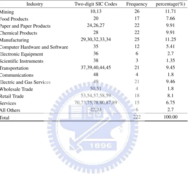
Table Ⅰ reports the distribution of our sample. Panel A shows the time distribution of our sample firms from 1981 to 2002. We can see that there are less sample firms from 1998 to 2002. Panel B presents the SIC code distribution of sample firms, and we find that firms concentrate on the industry of mining, manufacturing, chemical products, and paper and paper products.
Table Ⅱ displays the descriptive statistics of sample. Panel A shows the descriptive statistics of the debt maturity structure and discretionary current accruals. We can see that our sample firms have significant discretionary current accruals with mean of 2.4479%, and the mean of debt maturity is 81.8796%. Furthermore, we separate our sample into three groups by discretionary current accruals and find that as discretionary current accruals increase, the mean of debt maturity increase initially, but then decrease when discretionary current accruals are in relative high level. Panel B shows the descriptive statistics of sample of all other control variables. We can see that the mean of market-to-book ratio is 1.2860, the mean of firm size is 7.8153, the mean of abnormal earnings is -0.0837893%, the mean of asset maturity is
15.2810103, and the mean of leverage is 26.6558462%.
Table Ⅲ shows the matrix of Pearson correlation coefficients which presents the relationship between all exogenous variables and find that the multicollinearality is not a big problem of our regression.
4. Methodology
To analyze the relationship between debt maturity and earnings management, we use ordinary least squares (OLS) and two-stage least squares (2SLS) to estimate the regression model. In order to analyze the long-term performance of firms which may engage in earnings management, we use the method of Buy-and-Hold Abnormal Return (BHAR) and Fama and French’s three-factor model (1993).
4.1. Ordinary Least Squares Regression
Barclay and Smith (1995) use the percentage of debt that matures in more than three years as the dependent variable. Because we focus on the event of debt issuing in the research, we use the percentage of the amount of debt that matures in more than three years in previous year plus the amount of incremental debt in event date to the total debt in previous year plus the incremental debt in event date (DEBT3) as our dependent variable as follows:
debt l incrementa debt total debt l incrementa year than more in matures debt DEBT3 3 + + = (4.1.1)
Our independent variables include Discretionary Current Accruals (DCA) which is measured in previous, Market-to-Book ratio, Log of Firm Size, Abnormal Earnings, Term Structure, Regulation Dummy, Assets Maturity, and Tax rate. The ordinary least squares regression function is:
ε β β β β β β β β β β + + + + + + + + + + = ) ( ) (Re ) ( ) ( ) ( ) ( ) ( ) / ( ) ( 3 9 8 7 6 5 2 4 3 2 1 0 Maturity Assets Dummy gulation Rate Tax Structure Term Earnings Abnormal Size Firm Size Firm B M DCA DEBT (4.1.2)
4.2. Two-stage Least Square Regression
Because there might be the problem of endogeneity when DCA and leverage are used for explaining the debt maturity, we test the endogeneity between DEBT3 and DCA, DEBT3 and Leverage. We find that there exists the problem between DEBT3 and Leverage in our sample firms, so we form a simultaneous equation model and adopt two-stage least squares to
estimate our model as follows: ε β β β β β β β β β + + + + + + + + + = ) ( ) (Re ) ( ) ( ) ( ) ( ) / ( ) ( 3 8 7 6 5 2 4 3 2 1 0 Maturity Assets Dummy gulation Structure Term Earnings Abnormal Size Firm Size Firm B M DCA DEBT (4.2.1) (4.2.2) ) ( ) ( ) ( ) ( ) ( ) / ( ) 3 ( 6 5 4 3 2 1 0 Dummy Regulation Earnings Abnormal ity Profitabil Ratio Assets Fixed Size Firm B M DEBT Leverage β β β β β β β + + + + + + =
In the second-stage regression which takes DEBT3 as dependent variable, the Leverage in the function is the predicted Leverage estimated from the first-stage regressions. Difference with the model of ordinary least square, we delete the variable of TaxRatein the two-stage least square because we find that the impact of tax rate on debt maturity structure is uncertain in previous researches. According to our hypothesis, we expect that there should be positive relationship between debt maturity structure (DEBT3) and earnings management (DCA).
4.3. Buy-and-Hold Abnormal Return (BHAR)
Following Barber and Lyon (1997), and Mitchell and Stafford (2000), we calculate buy-and-hold abnormal returns (BHAR). We calculate 5-year BHARs for each sample firm that issues debt as follows:
∏
∏
= = + − + = T t T t t benchmark t i i R R BHAR 1 1 , , ) (1 ) 1 ( (4.3.1)where Ri,t is the month t simple return on a sample firm, Rbenchmark,t is the month t expected benchmarks return, T is the holding period. Three benchmarks are: (1) CRSP equally-weighted market portfolio; (2) CRSP value-weighted market portfolio; (3) a size and book-to-market matched control sample.
Then the mean buy-and-hold abnormal return is the weighted average of the individual BHARs of each firm as:
∑
= ⋅ = N i i i BHAR w BHAT 1 (4.3.2)where wi is the weight based on equally-weighted and value-weighted.
We separate our sample into three groups by their discretionary current accruals. “Aggressive firms” means firms with higher discretionary current accruals, and “Conservative firms” means firms with lower discretionary current accruals. We will calculate the abnormal returns of both aggressive firms and conservative firms by buy-and-hold method in order to compare their differences.
4.4. Three-factor Model of Fama and French
The other method that we use to measure the long-term stock performance is the three-factor model of Fama and French. According to Fama and French (1993), there are three stock-market factors: an overall market factor and factors related to firm size and book-to-market equity, and the regression of three-factor model is:
t p t p t p ft mt p p ft t p R R R s SMB h HML R , − =α +β ( − )+ + +ε , (4.4.1)
where Rp,t is the return of portfolio p in month t, Rft is the return on one-month Treasury bills in month t , Rmt is the return on a market index in month t , SMBt is the difference in the returns of a portfolio of small and big stocks in month t , and HMLtis the difference in the returns of a portfolio of high book-to-market stocks and low book-to-market stocks in month t . The intercept coefficient αp tests the null hypothesis that whether the average abnormal return is zero.
Similar to buy-and-hold abnormal return method, we also calculate the abnormal returns of both conservative and aggressive to examine the differences between these two parts.
5. Empirical Results
5.1. Results of Ordinary Least Square Regression
The results of ordinary least square regression are presented in Table Ⅳ. We can see that the coefficient of discretionary current accruals is positive and significant. Firms with higher discretionary current accruals will have higher DEBT3. It presents that the behavior of earnings management will affect the choice of debt maturity structure later.
As we can see, Table Ⅳ shows that the Firm Size is positive related to debt maturity structure significantly, and consistent with the results of Barclay and Smith (1995) and Smith and Warner (1979) that small firms will tend to issue more short-term debts to eliminate the conflicts between stockholders and bondholders. The sign of coefficient of tax rate is also positive and significant. It indicates that firms with high tax rate will tend to issue long-term debt. This result is consistent with Brick and Ravid (1985). The coefficient of M/B ratio which is the proxy of growth option is significantly positive and inconsistent with the result of Barclay’s (1995), but is consistent with the results of Datta, Iskandar-Datta, and Raman (2005) and the original finding of Stohs and Mauer (1995). As our prediction, the coefficient of Assets Maturity is positive but insignificant. However, inconsistent with our prediction, the coefficients of Term Structure and Regulation Dummy are negative, though they are insignificant. The coefficient of Abnormal Earnings is unexpected positive although it is insignificant.
5.2. Results of Two-stage Least Square Regression
Table Ⅴ shows the results of two-stage least square regression. Panel A presents the regression with DEBT3 as the dependent variable. From the empirical results in Table Ⅴ, we can find that the coefficient of discretionary current accruals (DCA) which is the proxy of earnings management is positive and significant at the 1 %, 5% and the 10% level. It supports
our hypothesis that firms with aggressive earnings management will have incentive to issue more debts with longer maturity.
The coefficients of Log of Firm Value and the square of Log of Firm Value are still positive and significant, and consistent with Barclay and Smith (1995). As our expectation, large firms will prefer to issue more long-term debt rather than small firms. The coefficient of Market-to-Book ratio is still positive but insignificant in this situation. We also find that the coefficient of Assets Maturity is still positive as our prediction but insignificant. The Abnormal Earnings is positive related to debt maturity structure and is inconsistent with our prediction but still insignificant. However, the coefficients of Term Structure and Regulation Dummy are both negative and inconsistent with previous prediction, although they are insignificant. Finally we can see that Leverage is positive related with debt maturity but still insignificant. Panel B shows the results of the second-stage regression with Leverage as the dependent variable.
5.3. Results of Long-term Performance of Buy-and-Hold Abnormal Returns
(BHAR)
Table Ⅵ reports the results of 5-year long-term performance of our sample firms by using the buy-and-hold abnormal returns method. Panel A shows the equally-weighted results. We can see that the abnormal returns of holding period from1-year to 5-year are all negative in firms with higher discretionary current accruals (defined as Aggressive firms). On the other hand, firms with lower discretionary current accruals (defined as Conservative Firms) also face positive long-term performance after debt issuing. Panel B shows the value-weighted results. Similar to equally-weighted results, we find that the abnormal returns of holding period from1-year to 5-year in aggressive sample firms are also negative, and the conservative firms have positive long-term performance in first two years then become negative from the third year. However, we can still find that the long-term performances of aggressive firms are
worse than conservative firms. Finally, panel C reports the results of abnormal returns using size and book-to-market matching firms as benchmarks. The result shows that almost all abnormal returns of each holding period are negative in aggressive firms, and conservative firms face positive long-term performance in first two years then become negative from the third year. As our prediction, the empirical results show that after firms with aggressive earnings management issue debt, they will have poor long-term performances in 5 years. This result is also consistent with the analysis of Teoh, Welch, and Wong’s (1998a).
5.4. Results of Long-term Performance of Fama and French Three-factor
Model
Table Ⅶ reports the results of 5-year long-term performance of our sample firms by using Fama and French’s Three-factor model. Panel A presents the equally-weighted results. From holding period 1-year to 5-year, we can see that all the abnormal returns of aggressive firms are negative. The long-term performances of conservative firms are also negative; however, they are still better than the long-term performances of aggressive firms. Panel B presents the value-weighted results. We can find that there are also negative abnormal returns of each holding period similar to equally-weighted results; however, the abnormal returns of conservative firms are negative in the first year after debt issuing and turn positive from the second year. The results of Fama and French’s Three-factor model also support our prediction that firms with aggressive earnings management will have poor long-term performances in 5 years after firms issuing debt.
From the empirical results of Fama and French’s three factor model, we can find that the abnormal return of value-weighted results is less significant than the equally-weighted results. According toLoughran and Ritter (1995), when the significantly abnormal return concentrate on small firms, the portfolio based on value-weighted may not reflect the real situation. Thus, we suppose that large firms may dominate the results of abnormal returns in our sample, and
6. Conclusion
Many previous literatures of debt maturity structure focus on agency problem, and they argue that firms will abate the agency problem by adjust their debt maturity structure. In our research, we focus on the asymmetric information between insider and outsider. We find that firms with aggressive earnings management will choose to issue more long-term debts. In order to raise enough fund more easily, firms will tend to conceal their true value and take earnings management. For avoid the outside monitors, firms with aggressive earnings management will have more incentive to issue debts with longer maturity. Furthermore, firms with aggressive earnings management issue long-term debt could prevent the higher cost of short-term debt issues if the real value of firms is revealed. Therefore, we can see that the higher the level of aggressive earnings management is, the higher proportion of the long-term debt in their capital structure is.
However, after outsiders realize the firms’ true value, they will lose their confidence in firms’ performance. Thus, in our study, we can see that the five-year long-term stock performances of these firms with aggressive earnings management after issuing debts are negative as our prediction.
To sum up, from our empirical results, the behavior of earnings management will affect the choice of debt maturity structure. Firms take aggressive earnings management will choose to have more long-term debt in their capital structure afterwards. In addition, these firms with aggressive earnings management will face poor long-term stock return performance after issuing debts because investors get the real information about firms’ performance.
References
Barber, Lyon, (1997), “Detecting Long-Term Abnormal Stock Returns: The Empirical Power and Specification of Test Statistics,” Journal of Financial Economics 43, 341-372. Barclay, M. J., and C.W. Smith Jr., (1995), “The Maturity Structure of Corporate Debt,”
Journal of Finance 50, 609-631.
Berger, Allen N., Marco A. Espinosa-Vega, W. Scott Frame, and Nathan H. Miller, (2005), “Debt Maturity, Risk, and Asymmetric Information,” Journal of Finance 60, 2895-2923. Brick, Ivan E., and S. Abraham Ravid, (1985) “On the Relevance of Debt Maturity Structure,”
Journal of Finance 40, 1423-1437.
Datta, Sudip, Mai Iskandar-Datta, and Kartik Raman, (2005), “Managerial Stock Ownership and the Maturity Structure of Corporate Debt,” Journal of Finance 60, 2333-2350. Diamond, Douglas W., (1991), “Debt Maturity Structure and Liquidity Risk,” Quarterly
Journal of Economics 106, 709-737.
Fama, Eugene F., and Kenneth R. French, (1993), “Common Risk Factors in the Returns on Stocks and Bonds,” Journal of Financial Economics 33, 3-56.
Flannery, Mark J., (1986), “Asymmetric Information and Risky Debt Maturity Choice,”
Journal of Finance 41, 19-37.
Guedes, Jose, and Tim Opler, (1996), “The Determinants of the Corporate Debt Issues,”
Journal of Finance 51, 1809-1833.
Gupta, Manu and L. Paige Fields, (2006), “Debt Maturity Structure and Earnings Management,” The Financial Management Association.
Healy, Paul M., and James M. Wahlen, (1999), “A Review of the Earnings Management Literature and Its Implications for Standard Setting,” Accounting Horizons 13, 365-383. Johnson, Shane A., (2003), “Debt Maturity and the Effects of Growth Opportunities and
Loughran, T., Ritter, J., (1995), “The New Issues Puzzle,” Journal of Finance 50, 23-51. Lyon, Barber, and Chih-Ling Tsai, (1999), “Improved Methods for Tests of Long-Run
Abnormal Stock Returns,” Journal of Finance 54, 165-201.
Myers, Stewart C., (1977), “Determinants of Corporate Borrowing,” Journal of Financial
Economics 5, 147-175.
Mitchell, Mark L., and Erik Stafford, (2000), “Managerial Decisions and Long-run Stock Price Performance,” Journal of Business 73, 287-329.
Smith, C.W., Jr., and Warner, J. B., (1979), “On Financial Contracting: An Analysis of Bond Covenants,” Journal of Financial Economics 7, 117-161.
Smith, C.W., Jr., (1986), “Investment Banking and the Capital Acquisition Process,”
Journal of Financial Economics 15, 3-29.
Stohs, Mark Hoven, and David C. Mauer, (1996), “The Determinants of Corporate Debt Maturity Structure,” Journal of Business 69, 279-312.
Teoh, Siew Hong, Ivo Welch, and T. J. Wong, (1998a), “Earnings Management and the Long-Run Market Performance of Initial Public Offerings,” Journal of Finance 53, 1935-1974.
Table ⅠⅠⅠⅠ
Distribution of Sample
The sample contains 222 firms which issue debts during the period from 1981 to 2002. The sample firms must have sufficient COMPUSTAT and CRSP data. Panel A reports the time distribution of sample firms, and Panel B reports the SIC code distribution of sample firms.
Panel A. Time Distribution
Year Frequency Percentage (%)
1981 15 6.76 1982 29 13.06 1983 23 10.36 1984 13 5.86 1985 23 10.36 1986 27 12.16 1987 10 4.5 1988 8 3.6 1989 7 3.15 1990 3 1.35 1991 12 5.41 1992 12 5.41 1993 15 6.76 1994 3 1.35 1995 7 3.15 1996 10 4.5 1998 1 0.45 1999 1 0.45 2001 2 0.9 2002 1 0.45 Total 222 100.00
Table ⅠⅠⅠ (Continued) Ⅰ
Panel B. SIC Distribution
Industry Two-digit SIC Codes Frequency percentage(%)
Mining 10,13 26 11.71
Food Products 20 17 7.66
Paper and Paper Products 24,26,27 22 9.91 Chemical Products 28 22 9.91 Manufacturing 29,30,32,33,34 25 11.25 Computer Hardware and Software 35 12 5.41 Electronic Equipment 36 6 2.7 Scientific Instruments 38 3 1.35 Transportation 37,39,40,44,45 21 9.45
Communications 48 4 1.8
Electric and Gas Services 49 21 9.46 Wholesale Trade 50,51 4 1.8 Retail Trade 53,54,57,58,59 18 8.1 Services 70,73,75,78,80,87,89 15 6.75
All Others 22,23 6 2.7
28
Table ⅡⅡⅡⅡ
Summary of Descriptive Statistics
The sample contains 222 firms which issue debts during the period from 1981 to 2002. Panel A shows the descriptive statistics of the debt maturity structure and discretionary current accruals (DCA). Panel B shows the descriptive statistics of sample of all other control variables. The M/B ratio is measured ad the ratio of market value of firm’s assets to the book value of assets. Firm Size is measured as the market value of total assets, and the market value of total assets is the book value of assets plus the market value of equity minus the book value of equity. Abnormal Earnings is measured as earnings per share in year t+1 minus earnings per share in year t, divided by the year t share price. Term Structure is the difference between the month-end yield of six-month T-bill and the month-end yield of ten-year government bonds. Asset Maturity is measured as the value-weighted average of the maturity of current assets and gross property, plant and equipment as (2.3.5). Tax Rate is measured as income tax expenses divided by pretax income. Leverage is measured as the ratio of total debt to market value of assets. Fixed Asset Ratio is measured as PPENT divided by book value of total assets. Profitability is measured as operating income before depreciation divided by book value of total assets.
Panel A. Descriptive statistics of DCA and DEBT3
DCA (%) Debt Maturity Structure (%)
Observations Mean Median Standard Dev. Mean Median Standard Dev.
Trisection 1 (DCA>2.00%) 74 11.7022 5.5225 22.0375 82.2734 85.8308 14.1760
Trisection 2 (-0.95%<DCA<2.00%) 74 0.4072 0.3634 0.7950 83.7569 87.2820 10.6760
Trisection 3 (DCA<-0.95%) 74 -4.7657 -2.6558 6.4421 79.6086 82.6173 14.1050
29
Table ⅡⅡⅡⅡ (Continued)
Panel B. Descriptive of independent variables
Variable Observations Mean Standard Dev. 25% Percentile Median 75% percentile
M/B 222 1.2860 0.4800 1.0156 1.1585 1.3911
Log of Firm Value 222 7.8153 1.6567 6.7247 7.9339 8.8901
Abnormal Earnings (%) 222 -0.0838 13.2602 -2.4 0.5657 2.7346
Term Structure (%) 222 2.1146 0.8763 1.56 2.205 2.66
Asset Maturity 222 15.2810 12.1241 7.1489 13.1728 20.5675
Tax Rate (%) 222 33.7974 78.9796 30.3492 37.8493 44.5231
Leverage (%) 222 26.6558 13.8767 17.8830 22.8819 34.1632
Fixed Assets Ratio 222 0.5027 0.2204 0.3359 0.5072 0.6932
30
Table ⅢⅢⅢⅢ
Pearson Correlations
Growth Firm Size Abnormal Term Asset Tax Rate DCA Leverage Fixed Assets Profitability Option Earnings Structure Maturity Ratio Growth 1 0.06893 -0.00805 -0.19875 -0.08216 0.06384 0.03106 -0.37982 0.04648 0.37455 Option (0.3066) (0.9050) (0.0029)* (0.2227) (0.3437) (0.6453) (<.0001)* (0.4908) (<.0001)* Firm Size 0.06893 1 0.11552 -0.11062 0.15636 0.17543 -0.15263 -0.23049 0.18207 0.19229 (0.3066) (0.0859) (0.1002) (0.0198) (0.0088)* (0.0229)* (0.0005)* (0.0065)* (0.0040)* Abnormal -0.00805 0.11552 1 0.08182 0.13407 -0.00178 -0.00723 0.10431 0.1704 -0.13243 Earnings (0.9050) (0.0859) (0.2247) (0.0460)* (0.9789) (0.9147) (0.1212) (0.0110)* (0.0488)* Term -0.19875 -0.11062 0.08182 1 0.01966 -0.06574 0.02305 0.06663 -0.03655 -0.05068 Structure (0.0029)* (0.1002) (0.2247) (0.7708) (0.3295) (0.7326) (0.3230) (0.5880) (0.4524) Asset -0.08216 0.15636 0.13407 0.01966 1 0.0132 -0.14789 0.06918 0.73718 -0.1015 Maturity (0.2227) (0.0198)* (0.0460)* (0.7708) (0.8449) (0.0276)* (0.3048) (<.0001)* (0.1316) Tax Rate 0.06384 0.17543 -0.00178 -0.06574 0.0132 1 -0.05646 -0.1769 0.04255 0.09436 (0.3437) (0.0088)* (0.9789) (0.3295) (0.8449) (0.4025) (0.0082)* (0.5283) (0.1612) DCA 0.03106 -0.15263 -0.00723 0.02305 -0.14789 -0.05646 1 -0.0379 -0.22709 -0.00541 (0.6453) (0.0229)* (0.9147) (0.7326) (0.0276)* (0.4025) (0.5743) (0.0007)* (0.9362) Leverage -0.37982 -0.23049 0.10431 0.06663 0.06918 -0.1769 -0.0379 1 0.00301 -0.42468 (<.0001)* (0.0005)* (0.1212) (0.3230) (0.3048) (0.0082)* (0.5743) (0.9644) (<.0001)* Fixed 0.04648 0.18207 0.1704 -0.03655 0.73718 0.04255 -0.22709 0.00301 1 0.13326 Assets Ratio (0.4908) (0.0065)* (0.0110)* (0.5880) (<.0001)* (0.5283) (0.0007)* (0.9644) (0.0474)* Profitability 0.37455 0.19229 -0.13243 -0.05068 -0.1015 0.09436 -0.00541 -0.42468 0.13326 1 (<.0001)* (0.0040)* (0.0488)* (0.4524) (0.1316) (0.1612) (0.9362) (<.0001)* (0.0474)*
Table ⅣⅣⅣⅣ
Ordinary Least Squares Regression Predicting Debt Maturity Structure
The table reports the OLS results of our sample. The dependent variable of this regression is DEBT3 and is regressed by DCA. Other control variables include market-to-book ratio, natural logarithm of firm value, abnormal return, term structure, regulation dummy assets maturity, and tax rate. White’s (1980) heteroskedasticity consistent t-statistics are in parentheses. ***, **, * indicate significant at the 1%, 5%, and 10% levels each.
Dependent Variable: Debt3
Variables Coefficient Standard Error Intercept 59.5160 13.9169 (4.2765)*** DCA 0.0819 0.0353 (2.3211)** Growth Option 3.5954 1.4903 (2.4126)** Firm Size 6.3717 3.5166 (1.811909)* (Firm Size)2 -0.4782 0.2236 (-2.1385)** Abnormal Earnings 0.0254 0.0881 (0.288341) Term Structure -0.9241 1.0037 (-0.9207) Asset Maturity 0.0118 0.0744 (0.1589) Regulation Dummy -4.4591 5.1510 (-0.8657) Tax Rate 0.0045 0.0078 (0.5702) R2 0.0583 Adj-R2 0.0183 Observation 222
Table ⅤⅤⅤⅤ
Two-Stage Least Squares Regression Predicting Debt Maturity
The table reports the 2SLS results of our sample firms. In panel A, the dependent variable of second-stage regression is DEBT3 and is regressed by discretionary current accruals (DCA). The DCA is the predicted DCA estimated in the first-stage regression. The Leverage is the predicted Leverage which is estimated from the first-stage regression. Panel B reports the results of the second-stage regression which dependent variable is Leverage. The DEBT3 is the predicted DEBT3 which is estimated from the first-stage regression. White’s (1980) heteroskedasticity consistent t-statistics are in parentheses. ***, **, * indicate the significant level of 1%, 5%, and 10%.
Panel A. Dependent Variable: Debt3
Variables Predicted Sign Coefficient Standard Error Intercept / 58.8360 21.6546 (2.72)*** DCA + 0.0820 0.0315 (2.60)*** Growth Option - 3.8629 3.3653 (1.15) Firm Size + 6.2419 3.6491 (1.71)* (Firm Size)2 - -0.4642 0.2240 (-2.07)** Abnormal Earnings - 0.0222 0.0936 (0.24) Term Structure + -0.9204 1.0154 (-0.91) Regulation Dummy + -4.4717 5.1017 (-0.88) Asset Maturity + 0.0106 0.0755 (0.14) Leverage + 0.0233 0.2544 (0.09) R-Square 0.0523 Adjusted R2 0.0121 Observation 222
Table ⅤⅤⅤⅤ (Continued)
Panel B. Dependent Variable: Leverage
Variables Coefficient Standard Error Intercept 75.1421 26.7867 (2.81)*** Debt3 -0.2314 0.2981 (-0.78) Growth Option -6.5149 2.7409 (-2.38)** Firm Size -1.6262 0.5402 (-3.01)***
Fixed Assets Ratio 2.8484 4.4647 (0.6380) Profitability -64.7305 10.9991 (-5.8851)*** Abnormal Earnings 0.0848 0.0663 (1.28) Regulation Dummy -2.1533 2.7994 (-0.77) R-Square 0.2761 Adjusted R2 0.2524 Observation 222
Table ⅥⅥⅥⅥ
Long-Term Stock Returns Performance of Buy-and-Hold Abnormal Returns
This table reports the 5-year long-term stock return performance which is measured by the method of buy-and-hold abnormal returns (BHAR). Panel A presents the equally-weighted abnormal returns. Panel B presents the value-weighted abnormal returns. Panel C presents the matching-firm adjusted abnormal returns where the matching firms are chosen on the basis of the size and the book-to-market ratio. ***, **, * indicate the significant levels at 1%, 5%, and 10%.
Panel A. BHAR (Equally-Weighted) Equally-Weighted
Holding Period (Year) 1 2 3 4 5
Whole Sample
Mean Abnormal Return -2.32% 2.96% 2.06% 2.36% 15.33% Cross-sectional t-stat -0.606 0.549 0.328 0.303 1.668* Skewness-adjusted t-stat -0.584 0.568 0.332 0.306 1.711*
Aggressive Firms
Mean Abnormal Return -9.95% -8.43% -17.23% -17.81% -2.02% Cross-sectional t-stat -1.188 -0.724 -1.775* -1.556 -0.147 Skewness-adjusted t-stat -0.986 -0.66 -1.631 -1.48 -0.147
Conservative Firms
Mean Abnormal Return 3.50% 7.69% 4.86% 3.30% 14.93% Cross-sectional t-stat 0.603 1.006 0.473 0.256 0.87 Skewness-adjusted t-stat 0.616 1.024 0.479 0.256 0.888
Panel B. BHAR (Value-Weighted) Value-Weighted
Holding Period (Year) 1 2 3 4 5
Whole Sample
Mean Abnormal Return 0.33% 1.18% -7.73% -15.97% -10.62% Cross-sectional t-stat 0.088 0.225 -1.216 -2.081** -1.175 Skewness-adjusted t-stat 0.089 0.229 -1.173 -1.975** -1.153
Aggressive Firms
Mean Abnormal Return -8.99% -10.67% -27.80% -38.20% -32.25% Cross-sectional t-stat -1.104 -0.945 -2.952*** -3.416*** -2.492*** Skewness-adjusted t-stat -0.924 -0.834 -2.559*** -3.065*** -2.378**
Conservative Firms
Mean Abnormal Return 5.56% 4.90% -5.47% -12.58% -6.41% Cross-sectional t-stat 0.955 0.688 -0.523 -0.984 -0.378 Skewness-adjusted t-stat 0.992 0.712 -0.518 -0.978 -0.375
Table ⅥⅥⅥ (Continued) Ⅵ
Panel C. BHAR (Matching firm) Matching Firms
Holding Period (Year) 1 2 3 4 5
Whole Sample
Mean Abnormal Return 0.49% -1.09% -1.76% -5.08% -6.71% Cross-sectional t-stat 0.224 -0.317 -0.473 -1.28 -1.504 Skewness-adjusted t-stat 0.227 -0.309 -0.461 -1.2 -1.422
Aggressive Firms
Mean Abnormal Return -5.76% -4.41% -8.58% -11.55% -15.95% Cross-sectional t-stat -1.54 -0.583 -1.524 -1.780* -2.488*** Skewness-adjusted t-stat -1.274 -0.529 -1.404 -1.556 -2.345**
Conservative Firms
Mean Abnormal Return 4.97% 0.19% -0.57% -2.33% -2.48% Cross-sectional t-stat 1.393 0.043 -0.098 -0.398 -0.312 Skewness-adjusted t-stat 1.441 0.043 -0.097 -0.396 -0.309
36
Table ⅦⅦⅦⅦ
Long-Term Stock Returns Performance of Fama and French Three-Factor Model Abnormal Returns
The table reports the 5-year long-term stock returns performance which is measured by Fama and French three-factor model. Panel A presents the equally-weighted abnormal returns. Panel B presents the value-weighted abnormal returns. The regression coefficients are estimated using weighted least squares to correct for heteroskedasticity. ***, **, * indicate the significant levels at 1%, 5%, and 10%.
Panel A. Fama and French Three-Factor Model (Equally-Weighted)
Equally-Weighted
Aggressive Conservative
Holding Period (Year) α β s h R2 α β s h R2
1 -0.0101 1.1524 0.6759 -0.0014 0.4676 -0.0031 1.3001 0.3832 0.4012 0.4089 (-2.03)** ( 9.90)*** ( 3.30)*** (-0.01) (-0.61) (10.23)*** ( 2.06)** ( 1.98)** 2 -0.0086 1.2474 0.6349 0.2267 0.6465 -0.0016 1.3201 0.3418 0.3445 0.5638 (-2.69)*** (17.07)*** ( 4.75)*** (1.64) (-0.48) (15.73)*** ( 2.54)*** ( 2.46)** 3 -0.0074 1.1951 0.6398 0.2109 0.6212 -0.0038 1.2938 0.3609 0.3447 0.6331 (-2.52)*** (16.76)*** ( 5.10)*** (1.61) (-1.42) (18.91)*** ( 3.30)*** ( 3.00)*** 4 -0.006 1.1692 0.7269 0.2331 0.6486 -0.0045 1.2941 0.2631 0.3996 0.6369 (-2.30)** (18.24)*** ( 6.57)*** ( 1.97)** (-1.85)* (20.56)*** ( 2.92)*** ( 3.78)*** 5 -0.0039 1.2007 0.5968 0.3116 0.6728 -0.0044 1.3019 0.3332 0.4581 0.6687 (-1.63) (20.78)*** ( 6.09)*** ( 2.85)*** (-1.96)** (22.56)*** ( 4.04)*** ( 4.79)***
37
Table ⅦⅦⅦ (Continued) Ⅶ
Panel B. Fama and French Three-Factor Model (Value-Weighted)
Value-Weighted
Aggressive Conservative
Holding Period (Year) α β s h R2 α β s h R2
1 -0.0039 1.0326 0.5904 -0.1126 0.3472 -0.0036 1.1241 0.051 0.2084 0.3074 (-0.66) ( 7.47)*** ( 2.43)** (-0.45) (-0.66) ( 8.14)*** (0.25) (0.95) 2 -0.0044 1.0783 0.3286 0.1146 0.4434 0.0031 1.1262 -0.1466 0.0581 0.4403 (-1.06) (11.48)*** (1.91)** (0.65) (0.84) (11.97)*** (-0.97) (0.37) 3 -0.0032 1.1503 0.3033 0.1346 0.5528 0.0017 1.098 -0.0972 0.1116 0.4837 (-1.02) (15.06)*** ( 2.26)** (0.96) (0.57) (13.90)*** (-0.77) (0.84) 4 -0.003 1.1414 0.3199 0.186 0.6291 0.0011 1.1599 -0.4199 0.1816 0.4866 (-1.20) (18.49)*** ( 3.00)*** (1.64) (0.36) (14.70)*** (-3.72)*** (1.37) 5 -0.0002 1.1397 0.0866 0.1962 0.6487 0.0018 1.2218 -0.3746 0.1759 0.5482 (-0.08) (20.67)*** (0.93) (1.88)* (0.66) (17.09)*** (-3.67)*** (1.49)