FISHERIESSCIENCE 2005; 71: 1256–1263
*Corresponding author: Tel: 886-223630846. Fax: 886-223633171. Email: i812@ntu.edu.tw
Received 14 May 2004. Accepted 8 June 2005.
Separation of the Taiwanese regular and deep tuna
longliners in the Indian Ocean using bigeye tuna
catch ratios
Ying-Chou LEE,1* Tom NISHIDA2 AND Masahiko MOHRI3
1Institute of Fisheries Science, National Taiwan University, Taipei 106, Taiwan, 2National Research Institute
of Far Seas Fisheries, Shizuoka, Shizuoka 424-8633 and 3National Fisheries University, Shimonoseki,
Yamaguchi 759-6595, Japan
ABSTRACT: Taiwanese longline (LL) fisheries operating in the Indian Ocean usually target albacore
tuna (ALB), swordfish (SWO) and yellowfin tuna (YFT ) using regular LL. Bigeye tuna (BET ), however, is targeted using deep LL. Thus, these two types of LL are considered to be different gears as they target different tuna species. Regular or deep LL fishing is defined by number of hooks per basket (NHB): regular LL if 6 ≤ NHB ≤ 10 and deep LL if 11 ≤ NHB ≤ 20. However, NHB information was available in only some of the recent LL data (1995–1999). This situation had caused problems of biased results in stock analysis in the past. Thus, the objective of our study was to explore an effective method to separate the two types of LL fishing by considering species composition. Some intervals of BET catch ratios were found to be effective in separating the regular and deep LL catches, i.e. 0.0 ≤ BET/(BET + ALB + SWO) ≤ 0.4 and 0.8 ≤ BET/(BET + ALB) ≤ 1.0, respectively. Using these two separators, the LL known data set (1995–1999) (learning data set) was classified. Correct classifi-cation occurred in 67.7% of the data, while 23.1% of the data were unclassified (11.9% due to zero catches and 11.2% due to classification into both LL types), and 9.2% were misclassifications. Then, using the methods developed, the LL unknown data set in the historical data (1979–1999) was clas-sified and nominal CPUE values were calculated for four species. The CPUE trends based on this study were likely to be more reliable than those of previous studies.
KEY WORDS: bigeye tuna catch ratios, Indian Ocean, regular and deep tuna longline,
separators.
INTRODUCTION
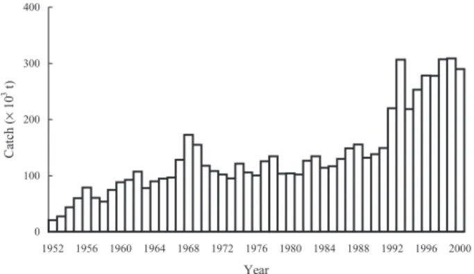
The industrial tuna longline (LL) fisheries in the Indian Ocean began in 1952 (Japan), 1954 (Taiwan), 1966 (Korea), and the 1980s (Indonesia, Sri Lanka and other developing countries).1 The total annual catches of all LL fisheries gradually increased from 20 000 t in 1952 to 170 000 t in 1967, then decreased and stabilized at 100 000–150 000 t in 1968–1991. After 1992, the total annual catches suddenly increased then stabilized at 200 000– 300 000 t in 2000 (Indian Ocean Tuna Commission (IOTC) database) (Fig. 1).
The LL was composed of a mainline and many branch lines with hooks at the terminal end. There
were two types of LL, i.e. regular LL and deep LL, which were defined by number of hooks between two floating balls (NHB). The regular LL had fewer NHB, while the deep LL had more NHB. The num-ber of NHB between regular LL and deep LL was slightly different depending on the country. The fishing depth of LL depended on the number of branch lines between two floating balls and the length of the branch lines (Fig. 2). Taiwanese fish-eries refer to the number of branch lines between two floating balls as a ‘basket’. Thus, the term bas-ket is used in Figure 2. If the LL forms a theoretical catenary curve, location of hooks can represent the depth of the hooks deployed, which implies the depth of fish caught or the swimming depth of fish. Around 1986, Taiwanese longliners in the Indian Ocean equipped with super-cold storage began catching bigeye tuna Thunnus obesus (BET) using deep LL at an operation depth of 50–200 m.2 Their target species was different from the Taiwanese
tra-ditional longliners (regular LL or shallow LL)2 with an operation depth of 50–120 m, primarily target-ing albacore Thunnus alalunga (ALB), swordfish
Xiphias gladius (SWO) and yellowfin tuna Thunnus albacares (YFT) in the Indian Ocean.
In the past, no NHB information had caused biases on standardizing the nominal catch per unit effort (CPUE) and on CPUE-based stock assess-ments for tuna and billfish resources, because all catch and effort data from both regular LL and deep LL had been pooled when analyzed.3 In order to conduct more realistic or unbiased tuna fisher-ies resource analysis, it was necessary to separate these two types of LL, regular LL and deep LL, because they targeted different species and need to be treated as different gears.
Under such circumstances, the Taiwanese gov-ernment decided to collect NHB information from fishing vessel logbooks in all three oceans starting from 1995. As a result, Taiwanese fishery biologists began developing the methods to separate regular LL and deep LL in the Indian Ocean.4–6 NHB
infor-mation and species compositions of the LL data were used to separate regular LL and deep LL and to estimate ALB CPUE. The results showed robust and smooth trends in both LL, but the trends with-out separation showed a sharp decrease in the combined (unseparated) LL, which is likely neither realistic nor accurate.4,5 In those studies, catch ratios of ALB/(BET + ALB) were used to distinguish between regular LL and deep LL.
However, it was necessary to take account of the BET, YFT, ALB and SWO catches with the appropri-ate separation method as these species were the primary species of Taiwanese LL fisheries in the Indian Ocean. Therefore, the objective of this study was to develop more general and accurate separa-tors in considering these four species. In this study, we used exploratory data analysis to develop a sep-aration method.
MATERIALS AND METHODS
Two data sets were used in this study: (i) regular and deep LL known data set (learning data set); and (ii) regular and deep LL unknown data set. The source of these data was the Overseas Fisheries Development Council of Taiwan. Table 1 shows the types of LL data. Approximately 40% of the Taiwanese LL set-by-set data for 1995–1999 included NHB information for the Indian Ocean, which can be used as the learning data set (Table 2). The regular and deep LL unknown data set (all data for 1979–1994 and 60% of the data for 1995–1999) did not contain NHB information. The aim of this work was to develop the most effective separators to classify LL unknown data sets into regular or deep LL, using these regular and deep LL known data sets. Data on BET, YFT, ALB and SWO were collected to look at unique species composi-tions observed in regular and deep LL. Then, LL unknown data were separated into regular or deep LL and classification powers (accuracy) of these separators were evaluated.
Fig. 1 Trend in tuna production from longline fisheries in the Indian Ocean (1952–2000).
0 100 200 300 400 1952 1956 1960 1964 1968 1972 1976 1980 1984 1988 1992 1996 2000 Year Catch ( ¥ 10 3 t)
Fig. 2 Schematic diagram of (a) regular, and (b) deep longline gears. One basket (a) (b) 0 100 300 200 m Float Float line Main line Hook line Branch Sea Surface
Table 1 Taiwanese longline data for the Indian Ocean (1967–1999) Year Area unit Time unit NHB† Information
1967–1978 5°× 5° Monthly Not available 1979–1994 5°× 5° Daily Not available
1995–1999 5°× 5° Daily available in 40% of data †
Number of hooks per basket.
Data source: Overseas Fisheries Development Council of the Republic of China.
RESULTS
Using the learning data set, the definition of regu-lar LL and deep LL by analyzing the NHB informa-tion was initially investigated. The range of NHB in this data set was 6–20, and formed a bimodal distribution (Fig. 3). The lower number of NHB denotes regular or shallow LL, while the higher number denotes deep LL. Based on the patterns of Figure 3 and also the fishing customs of Taiwanese LL fisheries, this study defined regular LL with 6 ≤ NHB ≤ 10 and the deep LL with 11 ≤ NHB ≤ 20.
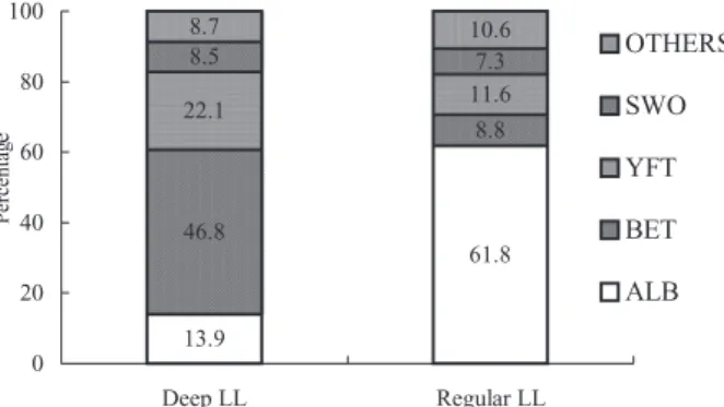
In order to investigate the most effective separa-tors, species compositions by regular and deep LL were further investigated using the learning data set (Fig. 4). In the regular LL, ALB was the major species (61.8%), while BET, YFT, and SWO were 8.8, 11.6 and 7.3%, respectively. In the deep LL, how-ever, the major species was BET (46.8%), while spe-cies compositions of ALB, YFT, and SWO were 13.9, 22.1 and 8.5%, respectively. Therefore, ALB may seem to be an effective indicator to separate
regu-lar and deep LL, as the compositions of these two gears were differentiated (61.8% vs 13.9%). How-ever, ALB was exploited only in the southern part of the Indian Ocean;7 hence, ALB was not considered to be a useful indicator for the entire Indian Ocean. Although BET compositions were less differenti-ated (8.8% vs 46.8%), BET was exploited in much wider areas in the Indian Ocean. In addition, BET was distributed in deeper waters (150–400 m) and it was the target species of the Taiwanese deep LL fisheries in the Indian Ocean. Hence, BET catch ratios were considered to be more effective than ALB catch ratios in separating regular and deep LL catches. Therefore, in this study, BET catch ratios were adopted as effective separators by combining catches of the other three species. The four BET ratios are defined as follows:
(1)
(2)
BET ratio (1) BET BET YFT =
+ BET ratio (2) BET
BET YFT SWO =
+ +
Table 2 Number of operations of Taiwanese tuna longline fisheries in the Indian Ocean by regular LL, deep LL and unknown LL (1995–1999)
Year
LL type Composition of the known
(regular or deep LL) data set (%) [(A) + (B)]/[(A) + (B) + (C)] Regular LL† (A) Deep LL‡ (B) (A) + (B) Unknown LL§ (C) 1995 4 330 2 786 7 116 12 238 36.77 1996 5 929 4 955 10 884 13 608 44.44 1997 3 948 5 547 9 495 16 008 37.23 1998 4 977 5 007 9 984 14 057 41.53 1999 2 955 6 156 9 111 12 278 42.60 Total 22 139 24 451 46 590 68 189 40.59 †Regular LL as 6 ≤ NHB ≤ 10. ‡Deep LL as 11 ≤ NHB ≤ 20.
§Unknown LL included in the data without NHB information and a few unclassified data as NHB ≤ 5 or NHB ≥ 21.
Note: (A) and (B) were used as the learning data sets in this paper.
Fig. 3 Frequency distribution of NHB in the learning data set from 1995 to 1999 (n = 46 590).
0 2000 4000 6000 8000 10000 6 7 8 9 10 11 12 13 14 15 16 17 18 19 20 Number of hooks per basket (NHB)
Number of records
Fig. 4 Species compositions of deep and regular lon-gline in the learning data set (n = 46 590).
13.9 61.8 46.8 8.8 22.1 11.6 8.5 7.3 8.7 10.6 0 20 40 60 80 100 Deep LL Regular LL Percentag e OTHERS SWO YFT BET ALB
(3)
(4) BET, ALB, YFT and SWO were the catches in num-ber of fish for bigeye tuna, albacore tuna, yellowfin tuna and swordfish, respectively. From these ratios, the best separator will be selected if the BET ratio has the highest value in the deep LL data set and if the BET ratio has the lowest value in the regular LL data set.
In evaluating these BET ratios, zero catches need to be excluded because the BET ratios cannot be calculated, i.e. BET = YFT = 0 for BET ratio (1), BET = YFT = SWO = 0 for BET ratio (2), BET = ALB = 0 for BET ratio (3), and BET = ALB = SWO = 0 for BET ratio (4).
The annual average BET ratio (3) = 0.922 was the highest and its standard error (SE) = 0.235 was the lowest in the deep LL data set, while the annual average BET ratio (4) = 0.225 was lowest and its
BET ratio (3) BET BET ALB =
+ BET ratio (4) BET
BET ALB SWO =
+ +
SE = 0.311 was lowest in the regular LL data set (Table 3). Therefore, BET ratio (3) was adopted as the best separator for the deep LL, and BET ratio (4) was adopted as the best separator for the regular LL.
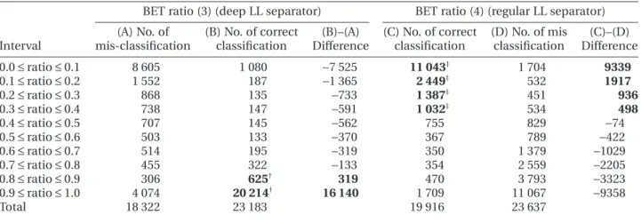
Then, using the learning data set, these separa-tors were further investigated by using a class interval of 0.1 to learn which intervals produced the most accurate classification powers as defined by correct and incorrect classification of deep and regular LL separated by BET ratios (3) and (4) (Table 4). The differences between correct and incorrect sets suggested that 0.8 ≤ BET ratio (3) ≤ 1.0 and 0.0 ≤ BET ratio (4) ≤ 0.4 were the most effective range intervals to separate deep and reg-ular LL, respectively, as these intervals produced correct classifications.
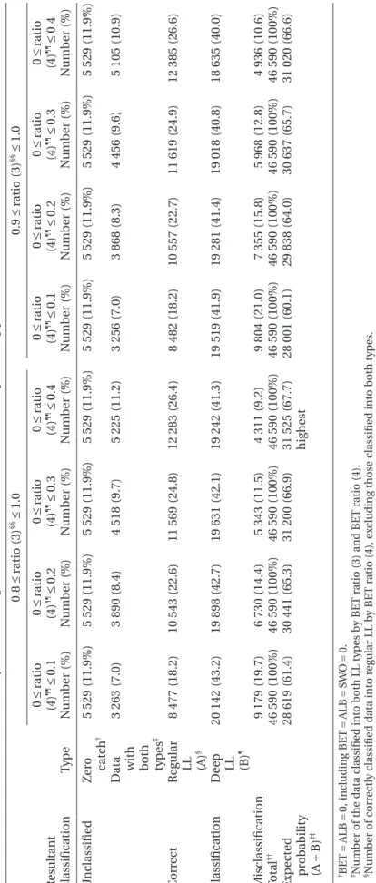
Using these interval ranges of two separators, which combinations of these intervals (by 0.1 interval) produced the highest correct classifica-tions were investigated. Eight cases as shown in Table 5 were investigated, i.e. two intervals for BET ratio (3) (0.8–1.0 and 0.9–1.0) and four intervals for Table 3 Results of four BET ratios in the learning data sets
BET ratio† Year Number of regular LL data sets Average value SE Number of deep LL data sets Average value SE (1) 1995–1999 18 908 0.594 0.399 24 065 0.712 0.280 (2) 1995–1999 19 682 0.427 0.371 24 357 0.620 0.286 (3) 1995–1999 18 322 0.357 0.400 23 183 0.922 0.235 (4) 1995–1999 19 916 0.225 0.311 23 637 0.772 0.293 † ; ; ; .
Note: The following zero catch cases are excluded in the calculations: data with BET = YFT = 0 for BET ratio (1), BET = YFT = SWO = 0
for BET ratio (2), BET = ALB = 0 for BET ratio (3) and BET = ALB = SWO = 0 for BET ratio (4).
BET ratio (1) BET
BET YFT =
+ BET ratio (2)
BET BET YFT SWO = + + BET ratio (3) BET BET ALB = + BET ratio (4) BET
BET ALB SWO
=
+ +
Table 4 Results of classification by BET ratio (3) (deep LL separator) and BET ratio (4) (regular LL separator) by class interval
Interval
BET ratio (3) (deep LL separator) BET ratio (4) (regular LL separator) (A) No. of mis-classification (B) No. of correct classification (B)–(A) Difference (C) No. of correct classification (D) No. of mis classification (C)–(D) Difference 0.0 ≤ ratio ≤ 0.1 8 605 1 080 −7 525 11 043‡ 1 704 9339 0.1 ≤ ratio ≤ 0.2 1 552 187 −1 365 2 449‡ 532 1917 0.2 ≤ ratio ≤ 0.3 868 135 −733 1 387‡ 451 936 0.3 ≤ ratio ≤ 0.4 738 147 −591 1 032‡ 534 498 0.4 ≤ ratio ≤ 0.5 707 145 −562 755 829 −74 0.5 ≤ ratio ≤ 0.6 503 133 −370 367 789 −422 0.6 ≤ ratio ≤ 0.7 514 195 −319 350 1 379 −1029 0.7 ≤ ratio ≤ 0.8 455 322 −133 354 2 559 −2205 0.8 ≤ ratio ≤ 0.9 306 625† 319 470 3 793 −3323 0.9 ≤ ratio ≤ 1.0 4 074 20 214† 16 140 1 709 11 067 −9358 Total 18 322 23 183 19 916 23 637
†total correct records = 20 839 and ‡total correct records = 15 911.
Note: Two separators were applied to the regular and deep LL known learning data sets (1995–1999) to classify into two group excluding zero catch data BET = ALB = 0 for BET ratio (3) and BET = ALB = SWO = 0 for BET ratio (4).
T
able 5
R
esults of the classification b
y
differ
ent r
anges of BET r
atio (3) and BET r
atio (4) pr oducing positiv e corr ect classification (r efer to T able 4) R esultant classification T ype 0.8 ≤ r atio (3) §§ ≤ 1.0 0.9 ≤ r atio (3) §§ ≤ 1.0 0 ≤ r atio (4) ¶¶ ≤ 0.1 N umber (%) 0 ≤ r atio (4) ¶¶ ≤ 0.2 N umber (%) 0 ≤ r atio (4) ¶¶ ≤ 0.3 N umber (%) 0 ≤ r atio (4) ¶¶ ≤ 0.4 N umber (%) 0 ≤ r atio (4) ¶¶ ≤ 0.1 N umber (%) 0 ≤ r atio (4) ¶¶ ≤ 0.2 N umber (%) 0 ≤ r atio (4) ¶¶ ≤ 0.3 N umber (%) 0 ≤ r atio (4) ¶¶ ≤ 0.4 N umber (%) U nclassified Z e ro catch † 5 529 (11.9%) 5 529 (11.9%) 5 529 (11.9%) 5 529 (11.9%) 5 529 (11.9%) 5 529 (11.9%) 5 529 (11.9%) 5 529 (11.9%) D
ata with both types
‡ 3 263 (7.0) 3 890 (8.4) 4 518 (9.7) 5 225 (11.2) 3 256 (7.0) 3 868 (8.3) 4 456 (9.6) 5 105 (10.9) C orr ect R egular LL (A) § 8 477 (18.2) 10 543 (22.6) 11 569 (24.8) 12 283 (26.4) 8 482 (18.2) 10 557 (22.7) 11 619 (24.9) 12 385 (26.6) classification D eep LL (B) ¶ 20 142 (43.2) 19 898 (42.7) 19 631 (42.1) 19 242 (41.3) 19 519 (41.9) 19 281 (41.4) 19 018 (40.8) 18 635 (40.0) M isclassification 9 179 (19.7) 6 730 (14.4) 5 343 (11.5) 4 311 (9.2) 9 804 (21.0) 7 355 (15.8) 5 968 (12.8) 4 936 (10.6) T otal †† 46 590 (100%) 46 590 (100%) 46 590 (100%) 46 590 (100%) 46 590 (100%) 46 590 (100%) 46 590 (100%) 46 590 (100%) E xpected pr obability (A + B) ‡‡ 28 619 (61.4) 30 441 (65.3) 31 200 (66.9) 31 525 (67.7) highest 28 001 (60.1) 29 838 (64.0) 30 637 (65.7) 31 020 (66.6) †BET = ALB = 0, including BET = ALB = SWO = 0. ‡N
umber of the data classifi
ed into both LL types b
y
BET r
atio (3) and BET ratio (4).
§N
umber of corr
ectly classified data into r
egular LL b
y
BET r
atio (4), ex
cluding those classifi
ed into both types
.
¶N
umber of corr
ectly classified data into deep LL b
y
BET r
atio (3), ex
cluding those classifi
ed into both types
.
††N
umber of the lear
ning data set (1995–1999).
‡‡E
xpected probability of corr
ect classification.
§§A
bbr
eviation of BET ratio (3).
¶¶A
bbr
BET ratio (4) (0–0.1, 0–0.2, 0–0.3 and 0–0.4). The best range appeared in 0.8 ≤ BET ratio (3) ≤ 1.0 and 0.0 ≤ BET ratio (4) ≤ 0.4. It was suggested that 67.7% of the data were correct classifications, while 23.1% were incorrect classifications (including 11.9% due to zero catches and 11.2% due to classification into both LL types) and 9.2% were due to misclassifica-tions (Fig. 5). This result implied that 67.7% of the unknown data can be correctly classified as regular or deep LL if the species composition of the unknown data is similar to those of the learning data set.
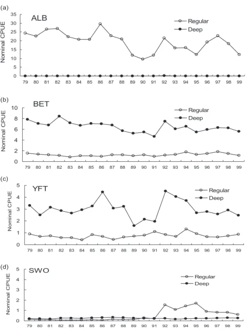
The nominal CPUE (number of fish per 103 fish-ing hooks) of ALB, BET, YFT, and SWO from 1979 to 1999 by regular and deep LL were calculated (Fig. 6). The nominal CPUE of ALB by the deep LL had lower values because ALB was not the target species for the deep LL, while the trend for the reg-ular LL was higher. In addition, the nominal CPUE of YFT by deep LL showed a stable trend except during 1986–1992, which showed high variation. However, that of BET showed a long-term decreas-ing trend from 1979 to 1991. The values in 1992 were similar to the levels of 1980, but after that, there was a smooth decrease from 1992 to 1999. YFT and BET were not the target species for regular LL, but still some catches were listed in the logsheets. The Taiwanese LL fisheries usually caught YFT using regular or shallow LL. However, the values of nominal YFT CPUE of deep LL were higher than those of regular LL. This is because deep LL usually operated in equatorial areas, while the regular LL operated in higher latitudes in the Indian Ocean. The former area had higher YFT density than that of the latter area.1 In addition, the regular LL targeted SWO beginning in 1992.
DISCUSSION
The CPUE trends of Indian BET based on this study were likely to be more reliable than that of a previ-ous study6 because of the following reasons. The CPUE trend of Indian BET decreased from 1979 to 1999, which was similar to that of the Japanese LL in the Indian Ocean.8 That is, LL for both countries exploited the same stock and thus the CPUE trends of both LL should show a similar trend. However, the decrease was opposite to that of a previous study,6 in which BET CPUE increased from 1991 to 1999. The results of that study may show higher BET CPUE values because of the ALB ratio (ALB/ (ALB + BET)) adopted for the studies.4,6 These authors separated the Taiwanese regular LL data when ALB ratio ≥0.82–0.97 for specific months in the high latitude area, ALB ratio ≤0.02 for all months in the equatorial area, and when ALB ratio ≥0.38 for all months in the south-western area; otherwise, all data were classified as Taiwan-ese deep LL. Among the three ALB ratios, the sec-ond one most probably misclassified many deep LL data with low BET catch as regular LL data. For example, one BET (individual only) was caught in a deep LL operation, where BET = 1 and ALB = YFT = SWO = 0. The calculated ALB ratio (ALB/(ALB + BET)) = 0 and thus this record is misclassified as regular LL. Misclassifications are a particular problem for catch data from the equatorial area. However, BET ratio (3) (BET/ (ALB + BET)) = 1 and thus the record is correctly classified as deep LL. In another scenario, one ALB (individual only) was caught in a regular LL opera-tion, ALB = 1 and BET = YFT = SWO = 0. The calculated ALB ratio (ALB/(ALB + BET)) = 1 and thus this record of data is correctly classified as regular LL. In addition, BET ratio (4) (BET/ (ALB + BET + SWO)) = 0 and thus the record is also correctly classified as regular LL. Therefore, BET CPUE values of the previous study6 have higher values because of misclassification of many deep LL with low catch as regular LL, and it showed an increasing trend from 1991 to 1999.
Total ALB catches from the Indian Ocean were between 8300 t and 38 500 t, and the average catch was about 19 200 t from 1979 to 1999. Among the total ALB catches, the Taiwanese catches were between 5800 t and 22 500 t, and the average catch was about 13 600 t in the same period.5 Thus, at least half of the Indian ALB catch came from the Taiwanese LL. As the maximum sustainable yield (MSY) of ALB is approximately 25 000 t,4–7 the stock status of Indian ALB should be robust but it fluctu-ated. Still, there was a sharply decreasing trend in the late 1990s owing to the high catch rate of the Taiwanese drift gill net fishery.9 Therefore, the
Fig. 5 Results of the classification BET ratio (3) and BET ratio (4) applied to the learning data set for 1995–1999 (n = 46 590). deep 41.3% regular 26.4% both 11.2% zero 11.9% mis-classfied 9.2% Unclassified (23.1%) Correct Classification (67.7%)
applied method can effectively separate Taiwanese LL data into deep and regular LL.
There are three reasons for the 32.3% incorrect classification. First, 10–20% of BET was supposed to be exploited by the deep LL but were misclassi-fied as regular LL, weakening the separation power of the method. Second, the LL shape was assumed to be a theoretical catenary. The depths of the deep LL should be deeper than that of the regular LL according to this assumption. However, sometimes the depths of the former may be not deeper than that of the latter underwater. Hence, if this assumption is not true, separation ability, espe-cially for BET ratio (3), is weakened. Misclassifica-tion errors occurred because deep LL caught fewer
BET. Third, there were zero catch situations, which made the separation impossible.
A possible solution was to substitute mis- or unclassified LL data. After the daily LL data was sep-arated into either regular LL or deep LL, resultant distributions of the two LL types were mapped. Iso-lated heterogeneous LL types found among the homogenous LL type on the map were considered to be misclassified data. This approach requires time to check all historical data. However, by con-ducting this error check, the incidence of mis- and unclassified data was minimized. Error checking was conducted by professional tuna scientists, tuna fishers, industry representatives and managers to acquire common understanding and agreement.
Fig. 6 Trend of nominal CPUE for (a) ALB, (b) BET, (c) YFT, and (d) SWO of LL unknown data clas-sified as regular and deep LL types by 0.8 ≤ BET ratio (3) ≤ 1.0 and 0.0 ≤ BET ratio (4) ≤ 0.4. Note that un-classified data with zero catches were excluded.
ALB 0 5 10 15 20 25 30 35 79 80 81 82 83 84 85 86 87 88 89 90 91 92 93 94 95 96 97 98 99 No m in a l CPU E Regular Deep BET 0 2 4 6 8 10 79 80 81 82 83 84 85 86 87 88 89 90 91 92 93 94 95 96 97 98 99 No m inal C P U E Regular Deep YFT 0 1 2 3 4 5 79 80 81 82 83 84 85 86 87 88 89 90 91 92 93 94 95 96 97 98 99 No m in a l CPU E Regular Deep SWO 0 1 2 3 4 5 79 80 81 82 83 84 85 86 87 88 89 90 91 92 93 94 95 96 97 98 99 No m in a l C PUE Regular Deep (a) (b) (c) (d)
Alternatively, the BET ratio method was consid-ered to be less useful in the ALB fishing area at high latitude, as there were less BET catches in these waters,10,11 which weakened the separation ability. Further, calculated BET ratios were probably vari-able because of seasons and subarea effects.
From Table 3, it is concluded that BET ratios including YFT, BET ratio (1) and BET ratio (2), were not effective. This is probably because YFT occa-sionally moved to waters deeper than 150 m, although it is usually distributed in regular LL depths (50–150 m),12,13 which probably weakened the separation ability.
For the LL unknown data set to separate into reg-ular and deep LL in 5°× 5° area on a monthly basis, the same criteria can be applied to separate regular and deep LL by considering the area and month as one sampling unit.
In this study, BET ratios were not considered by season and area. In the future, the seasonal and regional variations should be incorporated into the criteria in order to establish more practical separa-tors. In addition, exploratory data analyses were used in this paper, as the first step, to search for effective separators. However, it was suggested that the statistical method (modeling approach), such as a logistic generalized linear model or neural net-work analysis, needed to be developed to general-ize our method.14
In applying the developed methods to other LL data in different oceans and countries, the best effective separators may be obtained by examining species compositions and target species carefully as we did in our study, instead of simply applying the BET separators developed in this paper.
Finally, if regular and deep LL were separated accurately, it is expected that results of the tuna LL CPUE standardization and CPUE based stock assessments using models including virtual popu-lation analysis, age-structured production model, and a surplus production model incorporating covariates models, will become more reliable and robust.14
ACKNOWLEDGMENTS
We thank the staff of Overseas Fisheries Develop-ment Council of the Republic of China for provid-ing LL fisheries data in the Indian Ocean. We also appreciate Alejandro Anganuzzi (Indian Ocean Tuna Commission) who suggested the BET catch
ratio. The Council of Agriculture, Republic of China (91AS-3.3-FA-12) provided financial support.
REFERENCES
1. Lee YC, Liu HC. Standardized CPUE for yellowfin tuna caught by the Taiwanese longline fishery in the Indian Ocean, 1967–1998. IOTC/WPTT/00/26. 2000; 25.
2. Suzuki Z, Warashina Y, Kishida M. The comparison of catches by regular and deep tuna longline gears in the West-ern and Central Equatorial Pacific. Bull. Far Seas Fish. Res.
Lab. 1977; 19: 657–670.
3. Report of the IOTC ad hoc Working Party on methods, Sète, France, 2001; 20.
4. Lin CJ. The relationship between Taiwanese longline fishing patterns and catch compositions in the Indian Ocean. Master Thesis. Institute of Oceanography, National Taiwan University. 1998; 57 (in Chinese).
5. Chen CY. Stock assessment on the Indian albacore tuna.
IOTC/TWS/98/2/2. 1998; 21.
6. Hsu CC, Lee HH, Yeh YM, Liu HC. On targeting problem, partitioning fishing effort and estimating abundance index of bigeye tuna for Taiwanese longline fishery in the Indian Ocean. IOTC/WPTT/99/4. 2001; 23.
7. Liu HC, Lee YC. Stock assessment of albacore resource in the Indian Ocean. In: Hirano R, Hanyu I (eds). The Second
Asian Fisheries Forum. Asian Fisheries Society, Manila.
1990; 861–864.
8. Nishida T, Shono H, Okamoto H, Suzuke Z. Updated bigeye tuna (Thunnus obesus) resource analysis in the Indian Ocean- CPUE, ASPM (MSY) and Projections. IOTC/WPTT/
02/35. 2002; 11.
9. Lee YC, Liu HC. The virtual population analysis of Indian albacore stock. IPTP Collective Volumes 8: 107–116. In: Ardill JD (ed.). Proceedings of the Expert Consultation on
Indian Ocean Tunas, 5th Session. IPTP, Seychelles. 1993;
275.
10. Okamoto H, Chang SK, Yeh YY, Hsu CC. Standardized Taiwanese longline CPUE for bigeye tuna in the Indian Ocean up to 2002 applying targeting index in the model.
IOTC/WPTT/04/20. 2004; 23.
11. Nishida T, Lee YC, Hsu CC, Chang SK. Reviews and pros-pects on approaches reflecting actual dynamics of Taiwanese longline fisheries in CPUE standardization when number of hook per basket information is not available.
IOTC/WPTT/04/10. 2004; 8.
12. Mohri M, Nishida T. Consideration on distribution of adult yellowfin tuna (Thunnus albacares) in the Indian Ocean based on the Japanese tuna longline fisheries and survey information. IOTC/WPTT/00/5. 2000; 14.
13. Romena N. Factors affecting distribution of adult yellowfin tuna (Thunnus albacares) and its reproductive ecology in the Indian Ocean based on Japanese tuna longline fisheries and survey information. IOTC/WPTT/01/10. 2001; 97. 14. Report of the fourth session of the IOTC Working Party on