An optimal feedback control strategy for waste disposal management in agroecosystems

(1)

An optimal feedback control strategy for

waste disposal management in

agroecosystems

Chug-Min

Liao and Wen-Zer Lin

Department of Agricultural Engineering, National Taiwan University Taipei, Taiwan 10617, Republic of China

A dynamic model based on the linear systems theory is implemented in designing optimal feedback control strategies to efficiently manage waste disposal in agroecosystems. A physical and mathematical reuiew on the dynamic model leads to a residence time model describing the sojourn of waste disposal in an agroecosystem. Linear quadratic regulators (LQR’S) with output feedback control of a linear-invariant system are chosen for the design algorithm. Both impulse and step disturbances are taken into account and optimal proportional (P) and proportional plus integral (PI) feedback control strategies are synthesized. To illustrate this procedure the design is applied to manage residual phosphorus concentrations in a typical integrated pig/corn farming Jystem located in the south Taiwan region. Numerical data are obtained that could be used to design a controller minimizing fluctuations about a chosen equilibrium state. Numerical results from the model implementation show that the optimal selection of weighting parameters and the resulting costs vary with the desired equilibrium state. The designed optimal feedback controllers, when suitably tuned, give satisfactoy management of residual phosphorus concentrations in the pig farm. A sensitivity analysis is also performed to study the sensitivity of the objective function with respect to the controller gains. Feedback gains associated with residual phosphorus in the pig-subsystem are shown to be far more sensitive compared with that in corn-subsystem. 0 1997 by Elseuier Science Inc.

Keywords: agroecosystem, optimal feedback control, technical coefficient, waste disposal

1. Introduction

Agricultural agents influence each other, and sectors of an agroecosystem are interconnected. There are indirect as well as direct transmission paths and/or feedback loops in agroecosystems. Some indirect paths are due to the dynamics of the systems and may not be so obvious; thus counterintuitive phenomena may occur because of the complexity of these feedback loops.

Unless agroecosystems are treated as dynamic systems with the help of control and system theory it cannot adequately handle some of the phenomena associated with dynamic feedback loops.’ By examining the controllability and observability properties of dynamic systems, for instance the kinds of instruments that are needed to better stabilize the system or the new signals that are desirable to produce a more stable system, behavior can then be decided.

Address reprint requests to Dr. Liao at the Department of Agricul- tural Engineering, National Taiwan University, Taipei, Taiwan 10617, Republic of China.

Received 8 October 1996; accepted 5 December 1996.

Appl. Math. Modelling 1997, 21:165-174, March

An early attempt to use control theory with ecosystem management is found in Olsen’ who used analog comput- ers to model the flow of trace nuclides through ecosystems. Lowes and Blackwell and Boling and Van Sickle4 describe the application of engineering control theory to ecosystems. Mulholland and Sims’ used the stable com- partmental model to demonstrate in a general way how control theory could be used to achieve desired flow levels with linear and nonlinear models. Goh6 demonstrates why nonlinear control theory can be applied to only one or two variable systems. Kercher’ applied control theory to stable, dynamic, and linear models to find their frequency response to harmonic input. Hannon’ applied anticipatory and feedback control processes to an oyster reef ecosystem to stabilize the system after an unexpected external change. An ingenious concept in creating an agroecosys- tern in which a number of species coexist and are produced simultaneously has been described by Kok and Lacroix.’ They pointed out that it is possible to make agricultural production units autonomous by giving them sufficiently sophisticated control systems.

This present paper arises out of a collaborative project to investigate problems of waste disposal management in agroecosystems from the viewpoint of control engineering

(2)

Optimal feedback control for waste disposal management: C. -M. Liao and W. -2. Lin

and to show how ideas from the engineering sciences might be used to design feedback control laws for waste management. Management of one particular waste disposal is considered in detail to show the applicability of established techniques in control engineering. From a theoretical point of view it provides a framework for consideration of a large variety of energy/material ex- changes that affect the dynamic behavior of agroecosys- terns and offers additional mathematical tools to unravel the formal characteristics of whole agroecosystems.

From the practical engineering point of view optimal control theory is valuable mainly as a source of insight into the structure required for feedback controllers. A further insight is that dynamics serve as the purpose of estimation.

The purpose of this paper is to present initial consider- ations on the use of optimal control theory for designing an optimal feedback control strategy to efficiently manage waste disposal in an agroecosystem. Control logic developed for management of waste disposal will incorporate control logic algorithms used for other ecological factors in any other ecosystem. To illustrate this procedure the design is applied to manage residual phosphorus concentrations in a typical integrated pig/corn farming system located in the south Taiwan region. A sensitivity analysis is also performed to study the sensitivity of the objective function with respect to the controller gains.

2. Model structure

2.1 Model development

An input-output model can be used to develop a linear dynamic model describing the behavior of energy/material flow in agroecosystems. In input-output analysis” it is as follows: After observing xii, the flow of input from i to j, and qj, the total (gross) output of j, we form the ratio of input to output, xij/qj, denoted aij: aij =xij/qj; the ratio is termed a technical coefficient. Following the above mentioned concept an output dynamics in agroecosystems may be derived as follows.

There exists a pair of nonnegative matrices, [ A(t )] and [B(t)], in which [A(t)] is an irreducible (or indecompos- able) matrix for gross input coefficients, and [B(t)] is a partially reducible matrix of net output coefficients. [A(t)] and [B(t)] are both n-square matrices: [A(t)] = ((a,(t))), and [B(t)] = ((_bfj(t))); in which aij(t) is the gross input technical coeffrcrent of the ith resource in the jth process per unit mass of the jth resource available to the system, and bij(t) is the net output technical coefficient of the ith resource in the jth process per unit mass of the jth resource available to the system.

Two matrices of [ X(t)] and [Z(t)] are defined to achieve the construction of these technical coefficients. The ele- ments of [X(t)] = ((xii(t))) and [Z(t)] = ((zij(t))) are de- noted as the gross input and the net output of the. ith resource in the jth process at time t, respectively. A nonnegative, time-dependent, n-dimensional vector, {q(t)),

is then defined as follows: {q(t)} = (q,(t) q&) ... q,(t)}T; where yj(t) is the mass of the jth resource available to the system m the jth process at time t.

The matrices [A(t)] and [B(t)] are thus defined as technical coefficient matrices:

[A(t)1 =

[XWl{q-‘(t))

(1)

[B(t)1 =

[Z(t>l{qpl(t>l

(2)

In a time-invariant system [A(t)] = [A], and [B(t)] = [B]. If considering the fluctuations of the system [A(t)] and [B(t)] become:

[A(t)1 = [A,1 + [AAl

(3)

[B(t)1 =

[B,l + [ABI

(4)

where [A,] and [B,] are steady-state technical coefficient matrices of gross input and output and [AA] and [A B] are the technical coefficient changes in the [A,] and [B,] as the results of the fluctuation of the system, respectively.

Consider the dynamic behavior of available resources in an agroecosystem defined by given technical coefficients in which all resources are fully applied in all periods and all resources are produced in positive quantities. This means that the system is time invariant. Therefore the outputs of an agroecosystem in time t can be expressed by a first-order ordinary differential equation:

{4(t)] =

[B(t)l{q(t))

(5)

Equation (5) clearly shows the time path {q(t)) without explicit reference to the input matrix [A(t)]. In the special case of a time-invariant system the general solution of equation (5) is”:

{q(t)} =

exp([B,lt){q(O)l

(6)

where (q(O)) is the initial value vector of resource mass at t = 0.

The time path {q(t)} in that way depends on the values of the components of {q(O)) and on the structure of matrix [B,]. The concept of stability is extremely important, since every workable system must be designed to be stable. The elements of {q(t)} will remain bounded only if R,(A,) G 0 for all k, where A, is the eigenvalue of [B,].“,‘2

2.2 System control model

Under the modeling and control inseparability principle13 the modelling and control problems are not separable and are necessarily iterative. Hence a (model, controller) pair must be referred to as appropriate or inappropriate for each other. Therefore the capacity of-the controlled technical coefficient change (say, AGij, Ab,,) affects the limits imposed by the environment on the agroecosystem. The problem is thus the role of controlled technical coefficient change in enabling the agricultural agents to manage their environment to extend the life of resources in fixed supply and to minimize the damaging effects of waste disposal. Controlled technical coefficient change may be thought of

(3)

Optimal feedback control for waste disposal management: C. -M. Liao and W. -2. Lin as the deliberate application of residual quantities in new

combinations or forms.‘~‘4 Therefore technical coefficient change (Aaji,Abjj) in the general sense is a function of waste disposal.

The application of waste disposal for the agroecosys- tern to achieve a particular goal is a process that has all the characteristics of a controlled feedback process, i.e., the application of linear combinations of the resources, or state variables, of the agroecosystem to change it from an initial state to some other state. In other words, controlled technical coefficient change seeks to change the combination of resources available to the agroecosystem in future periods by changing the combination of resources ad- vanced now.

The description of technical coefficient changes as a control process is obtained by substituting equation (4) into equation (5),

{4(t)) = [B,l{q(t)l + [ABl{q(t)l (7)

If all technical coefficient changes are assumed to be controlled, equation (7) may be written in the form of a state-space realization of a linear dynamic system:

{4(t)) = [B,l{q(t)I +

[Ml{u(t)l

(8)

where {u(t)} is an n-dimensional control variables vector applied at the beginning of time f; [M] is an n-square control input matrix describing the technical coefficient changes in [B,].

The vector of control variables is the vector of residual quantities generated by the system in time t under the technical coefficient inherited from the previous time. The vector of waste disposal ({q,&t)}) has the following relations:

{qJ&)) =

([II - M,l){q(t)~

(9)

Therefore the vector of control variable ({u(t)}) can be defined as:

{u(r)) = {q&)1 =

HZ1 -

[~,ll~q(t)~ = Wl{q(t)l

(10)

If [H] = [[I] - [A,]] is nonsingular, the control input matrix [Ml can be written as, [Ml = [HI-‘[AL?].

When the control output of the system is defined to be the waste disposal in the system a complete description of the dynamics of available resources in an agroecosystem in terms of a state-space realization can be written as a linear dynamic system:

140)) =

[B,l{q(t)l+

[MlMt)~

(11)

{y(t)) =

[Cl{q(t)l

(12)

where {y(t)} is an output variable vector and [C] is a constant output matrix.

2.3 Residence time model

The genera1 solution of equation (11) is:

{q(t)} =

exp([B,lt){q(O)l

+

_/

‘exp([B,l(t - ~))[MIidt

-

T)]dT 0

(13)

The state variable at time (t +hX{q(t +h))) can be a transformed nonsingularity via a time-dependent transition probability ([P(h)]) by any other state variables at previous time ({q(t)}), and can be expressed asi’:

{q(t + h)) =

[P(h)l{q(t)I

(14)

As can be seen from equation (13), the solution of

{q(t + h)) is: {q(t + h)l =

(exp([B,lt)exp([B,lh)){q(O)}

+

_/‘exp([B,](t - r’))[M](~(t - 7’)) d+ 0 (15)

where T’ = r- h. If h is very small, a combination of equations (13) and (15) yields:

{q(t + h)l =

exp([B,lhNq(t))

(16)

In view of equations (15) and (16) an important rela- tionship between system matrix ([B,]) and transition probability matrix ([P(h)]) can be obtained as:

[P(h)1 = exp([B,lh)

(17)

Let Z’,$t) denote the element of

[P(t)l.

Then in an infinitesimal interval (t, t + dt) the mean time of waste disposal is in subsystem i, having started in subsystem j, before entering a subsystem, which is Pij(t)dt. The total mean time of waste disposal stays in subsystem i, having started in subsystem j, before entering a subsystem, and it is the (i,j)th element of [T] = /,“P(t)]dt. Integration of [T] may be obtained using the function of a matrix representation”:

Jrn [P(r)1 dr = /“expUB,lt) dt,

0 0

=

I( 0 I0 1/(27ri@ C

exp([

AIt)

x([hl[Zl

-

@,I)-‘dh dz, ) = 1/(2ni)$ (i= exp(]

*It)

dt)

x([hl[Zl

- [BJ-‘dh,

=

1/(277i)

(4)

Optimal feedback control for waste disposal management: C.-M. Liao and W.-Z. Lin

X

# c

-[Al-

= -[I?,]-’

‘([AI[Zl -

[B,l)-‘dh, where [P] = [PIT is the positive definite solution of the Riccati equation:

(18)

[PI = -[PI[B,l-

W,lTIPl

+mvflm-‘hwT~P1

- ts1,

[P(Q)]

= 0

where [A] is the distinct eigenvalue matrix of [B,], and C is the boundary of a domain containing the eigenvalues [A] of [B,], and they consist of a finite number of closed rectifiable Jordan curves. In the last step the contour C in the left-hand plane was chosen so that exp([A]t) approaches zero as 1 approaches infinity.

Therefore the row sum in [T], say the ith row, is equal to the mean residence time of waste disposal in subsystem i:

{i] = [TI{l) = -[&I_71) (19)

where {i} is the mean residence time vector of waste disposal in each subsystem.

3. Optimal feedback control synthesis

3.1 Optimal P control strategy

For the given linear control system in equations (11) and (12) an optimal control vector {r?(t)} is desired that will minimize the following quadratic cost function:

(20)

where [S] = [C]r[Q][C 1, in which [Q] is a positive semi- definite weighting matrix and [R] is a positive definite control weighting matrix.

To ensure that the controller can drive the system for a specified period of time the system must be controllable. On the other hand to control the system the performance with feedback must be monitored, thus the system must be observable. If the linear plant in equations (11) and (12) is observable, then [S] = [C]*[Q][C] is a positive semi-definite output-weighting matrix when [Q] is a positive semi-positive. Observability and controllability of the plant are guaranteed if and only if the following matrices:

[K(t)1 =

[m

[BITKITI

.** I (w’f[CIT],

[J(t)1 = [[Ml I [BI[Ml I .*.

I

[Bl”-wI

have rank n (i.e., ][K][ KITI # 0 and I[J][J]r I f O), respectively.r6

The solution of the optimal vector ({i;(t)}), which minimized equation (201, can be given by the following well- known expression:

{a(t)] =

-m-*MTIPl{~(t)~

(21)

If t approaches infinity and the system in equations (11) an d (12) is observable and controllable in the Kalman sense, the optimal control policy becomes a suboptimal controller design problem, and the suboptimal control vector in equation (21) can be expressed as:

(Li(t)] =

-m-1D41T~P*l~gt)J

(22)

where [P*] = [ P*lT is the unique, positive definite solu- tion of the following algebraic Riccati equation:

-1p*

I[~,1 - [mP*

1

+[P*IIMl[R]-l[M]TIP*l =o (23)

Equation (22) is the desired optimal feedback controller for the optimal linear quadratic regulator (LQR) with initial condition. This procedure can be seen as a modern control theory for designing a proportional feedback controller (P controller).

3.2 Optimal PI control strategy

The optimal LQR may be reformulated so that the resulting optimal feedback controller always brings the output state to a desired equilibrium condition in the presence of any finite constant disturbance (e.g., pesticide, pest, or food contaminants). Therefore when considering again equations (11) and (12), a more general form of system control model can be expressed as:

(4(t)] =

[B,J(q(t)) + [MHu(t)) + [DlW(t))

(24al

{q(O)) = (q(J),

b(O)) = b,)

(24bl

(y(t)) = [Cl(q(t))

(24~)

where [D] is a constant matrix and (W(t)) is subjected to constant disturbances,

K(t) = wj, i= 1,2 ,...,n @W

The quadratic cost function to be minimized may be rewritten as:

J=1 _{2 /,}If

_{(~ql=KWq~ + WfMW)}

_dt

₍₂₅₎

From a design point of view the cost function of equation (25) means the rates of change of control variables are penalized such that large values of control are prohibited indirectly rather than the control variables themselves.

(5)

Optimal feedback control for waste disposal management: C. 44. Liao and W. -Z. Lin

The derivative of equation (24) with respect to time yields:

@‘(t)l =

IB,1{4tt>l+ [Mllir(t)] (26a) {q(O)] = lqo], {U(O)] = lu,] (26b)

WXl =

[B,llq,l + [MllrGJ + [DlWf (26~)

{j(r)] = IClfr$t>l (26dI

and defines the following new variables:

(ol= Cd], lo] = {ti], l&]=(L)

Thus equations (24) and (26) can be reduced to the following pair of vector-matrix differential equation:

{4(t>l = (w(t)], {q(O)) = {q(J (27a)

{LJ(t)) =

LB,l{w(t)) + [Ml{6(t))

(27b)

fo(O)) =

1f$lb&J) -+ [~I{~~) + LDHW

(27~)

{y(t)) = ICl{q(t)) (27d)

{5(t)) = [Cllo(r)l (27eI

Equation (27) can be compactly expressed as:

15) = [C,Ibd

where

IT

11 CB,l=

@I

[Ma]= [&f]

1

1 {@IO))

= {~ii)

(28a) (28b)

Therefore equation (25) in terms of the new variables becomes:

where [S,] = diagE[Sl I [O]] = diag[~Cl~[~][Cl I [Oil. Matrix fs,] becomes a positive semi-definite since [S] is a positive semi-definite. Thus the original output LQR in equation (24) and (2.5) can be restated innequation (29).

An optimal control vector ({0(t)}) that minimizes equation (29) subject to a given linear system (28) can be found. This alternative problem is recognized as an LQR. The solution of the optimal control vector is given by the

well-known expression’3:

{i(t)) =

-~Rl-‘[~~l~[Pl{~(f))

(30) where [P] = [PIT is the positive definite solution of the Riccati equation:

[PI -

-fPltB,l

- k&lTP’l

-tI~l~~~lf~l-“~~~l~I~l-

[S,l,

[

P(tJ = 0

If system (28) is observable and controllable (i.e.,

[J(t)1

and [K(t)] are of full rank n), then as tf approaches infinity in equation (281, the LQR becomes a suboptimal controller design, and the suboptimal control vector in equation (30) becomes:

l$t)] = -[Rl-‘[M,lTIP*Il~(t)) (31) where [P*]

=

[P*]’ is the unique, positive definite solution of the following algebraic Riccati equation:

-[P*l[B,l -

[B,lTD’*l

Integrating equation (31) with respect to time gives:

+ULq,l+ [L2Lll~‘wT))d7

(32) a

The elements [Lij] in equation (32) are appropriately partitioned submatrices [ - [

R]-‘[~~l~[ P II.*

This is the desired optimal feedback controller to the original LQR as defined in equations (24) and (25). This procedure can be seen as a modern control theory method for designing the proportional plus integral feedback controller (PI controller).

Figure I

shows the structures of optimal P and PI control strategies for waste disposal management in the agroecosystem considered.

4.

Implementation

The objective of this section is to evaluate the performance of the optima1 P and PI feedback control strategies in managing the residual phosphorus concentrations in a typical integrated pig/corn farming ecosystem located at Yun-Lin, south Taiwan region (designated as the Y-L Farm). The feeding growing pigs were approximately 200 heads. The body weight of each growing pig was estimated to be 70 kg. The animals were fed a 70-80% ration, which was available for nutrient content, and a corn field of

18 ha was cultivated.

A farm system model is established to characterize the dynamic behavior of residual phosphorus in the Y-L Farm. There are two submodels in the farm system model:

(6)

Optimal feedback control for waste disposal management: C. -M. Liao and W. -Z. Lin

Table 1. Results of a field survey in the Y-L Farm (January 6, 1994-January 15, 1995) of net output and gross input parameters used in model implementation

I

PI CONTROLLER I 1

OJl

Figure 1. Structure of optimal P and PI control systems for residual flows management in an agroecosystem.

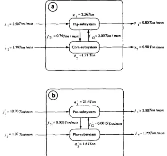
(1) the net output parameter model, formed by the Pig- subsystem, contains the elements of pigs/feedstuff, and the Corn-subsystem contains the elements of corn field/fertilizers/corn; and (2) the gross input parameter model, formed by Pro-subsystem, contains phosphor- feedstuff, and Pho-subsystem contains phosphor-fertilizer. Variables used in the farm system model to characterize the management of the residual phosphorus are adapted from the results of a long-term field survey (January 6, 1994-January 1.5, 1995) in the Y-L Farm and are listed in

Table 1. Figure 2 illustrates the farm system model and shows the transport pathways of net output and gross input parameters. Some assumptions are made to simplify the model: (1) no phosphorus concentration in pig waste is lost after the fermentation process and it is fully taken up by corn; (2) the percentage of nutrient content supplied to the Pig-subsystem as pig feedstuff is 100%; (3) the total phosphorus (T-P) concentration (ppm) is used to repre- sent the quantities of phospho-fertilizer and phospho- feedstuff; and (4) the nutrient content in feedstuff is represented by protein.

The first step in the performance investigations is to determine the steady-state coefficient matrices [A,] and [B,]. The construction of [A,] and [B,] is based on the results of the field survey in the Y-L Farm and the transport pathways of pig/corn subsystem and Pro- and Pho-subsystem in the farm system model (Table 2). Thus the changes take place in the matrices [A,] and [I?,] as the results of the fluctuation of the system, and [AA] and [ AB] are selected as diagonal matrices. The entries of [A A] and [A B] may be adapted from a report on annual products of pigs and corn based on Taiwan Agricultural Yearbook,17 i.e., [AB] = diag[OS, I] and [AA] = [O]. Ma- trix [H] can be determined from equation (lo), [HI = [Z] - [A,] = diag[OS, 0.331. Hence control input matrix

Net output parameters Pig-subsystem

1. Feedstuff, u, = 2.50 ton/man 2. Meat production, y, =0.85 ton/man 3. Swine waste contributed to Corn-subsystem,

f,, = 0.74 ton/man

4. Steady-state biomass of growing pig, 9, = 2.56 ton Corn-subsystem

1. Fertilizer requirement, uz= 1.79 ton/man 2. Food production, yz = 0.90 ton/man

3. Corn supplement to Pig-subsystem, f,,=2.00 ton/man 4. Steady-state storage of corn, 9z= 1.71 ton

Gross input parameters Pro-subsystem

1. Protein content, u; = 10.7 ton/man 2. Feedstuff, u, =2.50 ton/man

3. Protein contents contributed to Pho-subsystem,

f;, = 0.005 ton/man

4. Steady-state storage, 9: = 21.4 ton Pho-subsystem

1. Phosphorus content, rIz= 1.075 ton/man 2. Fertilizer requirement, uz= 1.79 ton/man

3. Phosphorus contents contributed to Pro-subsystem,

f;, = 0.0015 ton/man

4. Steady-state storage, 9;= 1.61 ton

[Ml can be calculated based on equation (11) as [Ml = [HI-‘[AB] = diag[l, 0.331. For simplicity [C] = [H] is assumed.

Having defined the matrices [A,], [B,], [AA], [ABI, [Cl, and [Ml the system control model of the residual

Figure 2. Transport pathways of (a) the Pig- and Corn-subsys- tems and tb) Pro- and Pho-subsystems in the farm system model based on Table 1.

(7)

Optimal feedback con&of for waste disposal management: C. -M. ho and W. -Z. Lin

Table 2. Construction of matrices [A,1 and [B,l for phosphorus flows dynamics in the farm system model based on Table 7 and

Figure 2

Pig- and corn-subsystems

1. State variable vector (ton): (9) = 1~~ q2)= (2.56 1.71) 2. Transport coefficient matrix (ton/man):

3. Input vector (ton/~on): !u)={u, u,)=i2.50 1.79) 4. Net output vector (ton/man): ( y) = (y, yz) = (0.85 0.90)

Pro- and Pho-subsystems

1. State variables vector (ton): (q’)=(;~ &1=(21.4 1.61) 2. Transport coefficient matrix (ton/man):

LF.I=[ ;: X~]=[ -;g; _?%:“I

3. Input vector (ton/man): fu’)=fu; u;l=(10.7 1.07) 4. Gross output vector (ton/mot+ [u) = {u, u2) = l2.50 1.79)

_:::;I

[A,]= [::: :i:] = [

o.z23

0.00093 0.67 _I

blj =

-h,,

+fi,)/q,, i =j Cu:, +fi;)/qj, i =j

Aj/Sjvi+.i

, aij =

f:,/qj, i +.i

phosphorus dynamics in the Y-L Farm can then be obtained based on equations (11) and (12) as:

-6E -:::8i]jl(:}+[: 00,3]{,“i} (33a)

i::) = Loi0 0.!3]{ z) (33b)

Table 3 lists the qualitative analysis results of the system control model, including stability, controIlabiIity/observa-

Table 3. Results of qualitative analyses of the system control model Stability analysis 1. system matrix: [B,l= t - “” 1.17 0.29 -7.48 I 2. eigenvaluevector: {hj=(h, A,)=[-2Y22 -1.02) Controllability and observability analysis

IJl=IlMl I IB,I1MIl= I :,

~~][~]~I

+

z2 - 0.29 l .76 -47.30 37.44

1 f

0, rank=n

rKl=rrCI’I~B,l~~CI’I= 1 “06 0.33 O -0.59 -0.88 -0.49 0.1 I ’ I[~l[Kl~l+ 0, rank=n

Residence time analysis

lT,= _LB,l-, = 0.65 I

0.52 0.13 _{0.78 1}

bility, and residence time analyses. Table 3 shows that the state stability and controllabili~/obse~abili~ of the system are verified, while residence times of residual phosphorus concentration are 1.17 and 0.91 months, respectively, in the Pig- and Corn-subsystems.

Next the effects of weighting matrices [S] and [RI in the quadratic cost function are investigated. Usually [s] and IR] are selected to be diagonal in order to secure the system’s robustness properties.”

The corresponding scalar expression of the quadratic cost function for the Y-L Farm in optimal P and PI control systems can be attained by equations (20) and (25):

Because q? and u’ are of same orders of magnitude, approximate scaling factors are not necessarily used in the selection of IS] and [RI.‘? Because no general criterion could be found it is assumed that uf and ti’ are of the same magnitude.

The elements in weighting matrices in equation (34) have the following relations: s,,q: =~~~qz and r,,uF = r,,uz, as a result, fI1 =sz2 and rli =rz2. Thus it is only necessary to adjust s,, and r,, while keeping sz2 and rT2 fixed. In this work rll is set at 1 and only s,, is varied.

The optimal P controller can be expressed by equation (22):

where [K,] is a proportional feedback gain matrix. When carrying out the matrix multiplication equation (35) can be written as:

The matrix [K,] contains four feedback gains, kll, k,,, kZ1, and kz2, which are computed for the optimal P controller. Similarly let [Kpl] be a proportional pfus integral feedback gain matrix that contains eight feedback gains (k,,, k,,, k,,, k,,, k,, ,..., k2J for the optimal PI controller. The ootimal PI controller can then be pressed by equatidn (32): ex- kn kn k,, k,, k,, k,, _I< ,fa2f7) d7 J Q,(t) , &(t) ~~)r=~T~(1)=~0.65+0.52=l.17 0.13+0.78==0.91) (37a)

(8)

Optimaf feedback control for waste dispcsai menageme~t: C. 44. Liao and W. -Z. Lin

where

k

11

42 43 k‘l

k

21

k22 k,, k24

I =

[f&,1

(37b)

Table 4 lists the elements of P and PI feedback gain matrices of [K,] and [Kp,] varied with si, values.

The model analyses were done in MATLAB: Control System Toolbox. Figwes 3 and 4 show the simulated time- history of error (i.e., the difference between actual and desired values) responses of residual phosphorus concentrations in the Pig-subsystem under no control and optimal P and PI control efforts at si, = 1, 5, 10, and 100. Figure 5 gives the simulated responses of residual phos- phorus concentrations in the Pig- and Corn-subsystems under no control and an optimal PI control effort at s ii = 1, 10, and 100, with the desired equilibrium value shown 80 ppm. These figures indicate that the responses were governed by the parameter si,. The success of these manipulations on control efforts can be achieved by ad- justing the specified performance bounds for output and input variables to properly select the weighting matrices.

Figure 6 shows the simulated time-histo~ of error responses of residual phosphorus ~ncentrations in the Pig-subsystem under no control and an optimal PI control action subjected to the constant disturbances w = 3.5, 5.5, and 7.5 at si, = 1.0. Figure 6 also shows conflicting re- quirements between what is needed for steady-state stability and what is needed for noise rejection, as with velocity feedback in conventional position-control systems.

The evaluation of the optimal feedback control strategies presented above concludes that a satisfactory control of residual phosphorus concentrations in the Y-L Farm can be reached when the optimal feedback controllers are suitably tuned. In addition, numerical results from the

Table 4. The elements of P and Pi feedback gain matrices of

lK,l and [K,,l varied with s,, values 1. s,,=l [K,l=

1

0.0280 0.0390 0.0010 1 ’ 0.9560 [K,,l= 1 0.3189 0.2340 0.0126 0.9442 0.9964 0.0844 -0.0844 0.8975 I 2. s,,=5 tK,l= [ 0.1636 0.6396 0.0200 0.1956 1 * IK,,l= [ 0.6774 0.0440 0.9986 - 1.2996 0.3914 0.0535 _0.05350.8869

1

3. s,,=lO ‘Kpl= [ 1 .0116 2.3362 0.0730 0.3752

1 ’

[K,,l= I 0.9997 2.1129 0.0669 0.3546 0.9999 0.0135 -0.0135 0.9763 1 4. s,,=lOO [K,l= 1 5.5494 7.0568 0.2205 0.6462 1 ’ [K,,I= I 0.6774 1.2996 0.0440 0.3914 0.9986 0.0535 -0.0535 0.7988

1

0.35 0.3 2 4 0.25 2 'Z 3 0.2 E p 8 0.15 r 2 e 0.1 8 e 0.05 oi I 0 2 4 6 8 IO I2 Time OmuW

Figure 3. Simulated time-history of error responses of residual

phosphorus concentration in the Pig-subsystem under no con- trol and optimal P control strategies at s,, =l, 5, 10, and 100.

simulation show that the optimal choice of tuning parameter s,, and the resulting costs vary with the desired equilibrium state.

Sensitivity analysis for system parameters is performed to provide information concerning the accuracy require- ments of the various feedback gains during the actual design of the individual controllers. The term “sensitivity” means relative changes in the measures of merit caused by given changes in the various feedback gains.

Equation (37) is valid for the optimal PI control. The controller parameters that shall be concentrated on are the eight feedback gain elements (k, Ir k,,, . . . , k,), which will be rearranged as k,, k, ,..., k,, respectively. Table 5 summ~izes the results of sensitivity analysis of the optimal PI controller gains. The nominal values of k, shown are the optimal values determined via the development of feedback control synthesis for the system considered (Tu- bfe 4). The sensitivity of the objective function with re-

Figure 4. Simulated time-history of error responses of residual

phosphorus concentration in the Pig-subsystem under no con- trol and optimal PI control strategies at s,, = 1, 5, 10, and 100.

(9)

Optimal feedback control for waste disposal management: C. 44. Liao and W. -Z. Lin x200 0.6 05 04 m value = 80 ppm 0.3 02 01 01 I 0 2 4 6 0 IO I? Time (month)

Figure 5. Simulated responses of residual phosphorus concen- tration in the Pig- and Corn-subsystems under no control and optimal PI control actions at s,, = 1, 10. and 100.

spect to the feedback gain elements may be represented as the magnitude of a symmetry matrix [M,,]. Matrix [M,;] may be referred to as a relative sensitivity coefficient matrix. The magnitude of [Mii] can be defined by the maximum eigenvalues of [M,,]: ]l[M,,]]] = max(lA,(,Ihz] ,..., IAJ where hi, i= 1,2 ,..., n are the eigenvalues of [Mii]. Matrix [M,,] and I][M,,l II are determined according to the work developed by Pagurek.‘s

Table 5 shows that the objective is about lo5 times more sensitive to the feedback gains associated with q1

than that to those associated with q2. This suggests that great care has to be exercised in maintaining the feedback gains of residual phosphorus in the Pig-subsystem at their nominal values because the optimal performance of the overall control scheme depends more on those nominal values than those in the Corn-subsystem.

It is difficult to generalize the effect of changing s,i upon the various gain sensitivities. Individual case studies may have to be undertaken to study the effects of weight-

0 2 4 6 a IO 12 Tie (month)

Figure 6. Simulated time-history of error responses of residual phosphorus concentration in the Pig-subsystem under no con- trol and optimal PI control strategies subject to constant distur- bances w=3.5, 5.5, and 7.5 at s,, =l.O.

Table 5. Results of sensitivity analysis of optimal PI controller gains s,,=l.O k,=0.3189(11597.15)* k, = 0.9964 (16780.53) k,=0.2340 (16086.4) k,=0.0844 (17010.06) k,=0.0126(1.12) k,= -0.0844 (1.63) k,=0.9442 (2.004) k, = 0.8975 (0.76) S ,,=lO k, =0.9997 (3147.5)* k, = 0.9999 (29023.7) k, = 2.1129 (11009.67) k,=0.0135 (3147.5) k,= 0.0669 (6.4) k,= -0.0135 (5.06) k,=0.3546 (0.095) k, = 0.9763 (0.95) *Magnitude of [M,,l.

ing factors on gain sensitivities, since the above results are only those of a particular study. In designing a control system the designer cannot treat all the parameters (gains) of the control system with equal importance, for all the possible parameter variations some are much more critical than others in determining whether the complete system can be expected to meet the given specification. Therefore special attention must be paid to these critical parameters (gains).

5. Conclusions

This paper results from a collaborative project to investigate waste disposal management in agroecosystems from the viewpoint of control engineering. By considering one particular problem it shows that engineering methodology can be used to illuminate problems in managing waste disposal problem in agroecosystems. The chosen control problem was that of regulating a single waste to a specified equilibrium state perturbed by finite constant fluctuations. Economic and political factors were not explicitly considered. Extension of the work to include them could be a topic for further research.

The control engineering approach starts by specifying a mathematical model that describes essential features of available resource dynamics in agroecosystems. The model relates variables representing the amount of commodity

(q) and residual concentration (~1. The objective of managing waste disposal is modelled as a requirement to minimize a cost function in a form of a weighted sum of squared, normalized fluctuations in q and CL The weighting coefficient sii serves as a tuning parameter in the resulting control law.

Specific results from the engineering approach to this particular problem confirm that feedback control can be satisfactory in providing safe regulation of residual concentrations over a wide range of target values. Any attempt to sustain high effort in maximizing sustainable

(10)

Optimal feedback control for waste disposal management: C.-M. Liao and W.-Z. Lin

yields is liable to break stabilities of residual concentration dynamics in an agroecosystem. As a result a workable agroecosystem is threatened (or jeopardized) unless feedback control is implemented. More generally this paper has shown that the methodology of control engineering can provide a scientific framework for discussing problems of managing waste disposal in an agroecosystem. Both fields are concerned with control in the presence of uncer- tainty. Management of a toxic residual concentration may require that decisions be made in the presence of uncer- tainty. Feedback is indicated to guide such decisions. Control engineering provides established techniques for analysis, design, and implementation of practical feedback controllers.

Acknowledgments

The authors wish to acknowledge the financial support of the National Science Council of Republic of China under Grant NSC-86-2313-B-002-094.

References

Walters, C. Adaptirv Management of Renewable Resources.

Macmillan, New York, 1986

Olsen, J. Analog computer models for movement of nuclides through ecosystems. Radiology, Proceedings of the First National Symposium, Cola. State University of New York, Rheinhold Publishing, New York, 1961, pp. 121-125

Lowes, A. and Blackwell, C. Applications of modern control theory to ecological systems. Ecosystems Analysis and Prediction,

ed. S. A. Levin, SIAM, Philadelphia, 1975, pp. 299-305

4. 5. 6. 7. 8. 9. 10. 11. 12. 13. 14. 15. 16. 17. 18. 19.

Boling, R. and Van Sickle, J. Control theory in ecosystem management. Ecological Analysis and Prediction, ed. S. A. Levin, SIAM, Philadelphia, 1975, pp. 219-229

Mulholland, R. and Sims, C. Control theory and regulation of ecosystems. Systems Analysis and Simulation in Ecology, ed. B. C. Patten, SIAM, Philadelphia, 1976, pp. 299-305

Goh, B. The usefulness of optimal control theory to ecological problems. Theoretical Systems Ecology, ed. E. Halfon, Academic Press, New York, 1986, pp. 385-399

Kercker, J. Closed-form solutions to sensitivity equations in the frequency and time domains for linear models of ecosystems.

Eco. Modelling 1983, 18, 209-212

Hannon, B. Ecosystem control theory. J. Theor. Biol. 1983, 121,

417-437

Kok, R. and Lacroix, R. An analytical framework for the design of autonomous, enclosed agro-ecosystems. Agric. Systems 1993, 43, 235-260

Miller, R. E. and Blair, P. D. Input-Output Analysis: Foundations and Extensions, Prentice-Hall, Englewood Cliffs, NJ, 1985 Chen, C. T. Linear System Theory and Design. Holt, Rhinehart and Winston, New York, 1984

Liao, C. M. and Feddes, J. J. R. Mathematical analysis of a lumped-parameter model for describing the behavior of airborne dust in animal housing. Appl. Math. Modelling 1990, 14, 248-257

Skelton, R. E. Dynamics Systems Control. Wiley, New York, 1988 Georgescu-Roegen, N. The Entropy Law and the Economic Pro- cess. Harvard University Press, Cambridge, MA, 1971

Zadeh, L. A. and Desoer, C. A. Linear System Theory. McGraw- Hill, New York, 1963

Palm, W. J. Modeling, Analysis and Control of Dynamic Systems.

Wiley, New York, 1983

Taiwan Provincial Government. Taiwan Agricultural Yearbook.

Department of Agriculture and Forestry, Taiwan Provincial Gov- ernment, 1994

Anderson, B. 0. D. and Moore, J. B. Optimal Control: Linear Quadratic Method. Prentice-Hall, Englewood Cliffs, NJ, 1990 Pagurek, B. Sensitivity of the performance of optimal linear control systems to parameter variation. Int. .I. Control 1965, 1, 33-45