邊界元素法之改良

行政院國家科學委員會專題研究計畫 成果報告

邊界元素法之改良

計畫類別： 個別型計畫 計畫編號： NSC91-2611-E-002-008-執行期間： 91 年 08 月 01 日至 92 年 07 月 31 日 執行單位： 國立臺灣大學工程科學及海洋工程學系暨研究所 計畫主持人： 黃維信 計畫參與人員： 葛家豪,劉得力 報告類型： 精簡報告 處理方式： 本計畫可公開查詢

中

華

民

國 92 年 8 月 13 日

行政院國家科學委員會專題研究計畫成果報告

邊界元素法之改良

The Improvement of Boundary Element Methods

計畫編號：NSC 91-2611-E-002-008

執行期限：91 年 8 月 1 日至 92 年 7 月 31 日

主持人：黃維信 國立台灣大學工程科學及海洋工

程研究所

計畫參與人員:劉得力 國立台灣大學工程科學及海洋工

程研究所

計畫參與人員:葛家豪 國立台灣大學土木工程學研究所

一、中文摘要 本研究著重於傳統邊界元素法中奇異積分過程之改良。當採用二次或更高階 元素應用於二維邊界元素法時，往往必須採用對數積分法以解決對基本解時所遇 到的奇異問題。本文則進一步將此一過程改良，透過解析的方式直接處理奇異積 分問題，如此將使得數值積分過程中，僅需採用傳統高斯積方法，就可以得到準 確之計算值。 關鍵詞：邊界元素法，邊界積分式，奇異積分 Abstr act

To integrate singular integrals on plane boundary elements, the logarithmic Gaussian quadrature is commonly used and suggested in many textbooks. Due to this special scheme, more and complicated calculating efforts are required while codes programming. In this study, a simple and efficient method that only adopts the standard Gaussian quadrature is presented here to solve such a problem.

Integration

二、緣由與目的

In the past two decades, the boundary element method (or BEM) has become a very popular method for engineers and scientists. BEM has widely been introduced in many textbooks and lectures. One of characteristics in BEM is that there are spiny singular integrals in elements that frequently confuse many researchers or students at the beginning.

The singular integrals of BEM occur at the integration of a fundamental solution or its derivatives. For example, in a plane potential problem, all textbooks mentioned the solving procedure and the numerical integration for the fundamental solution. However, most textbooks just introduced constant and linear elements only, because their analytical expressions can easily be derived on a local element. For higher-order elements, it is very difficult to derive analytical formulas for those singular integrals. In the literatures, many methods were proposed to handle such a singular integral. However, most of them are not straightforward. In a plane case, the most straightforward technique for treating the singular integration is so called the logarithmic Gaussian quadrature. This scheme was mentioned that it could perform a better numerical integration than the standard Gaussian quadrature did [1,2]. However, this scheme is a little complicated for program coding.

In this paper, a simple technique is proposed to handle the singular integral in an arbitrary-order element. This idea has been known for a long time such as Kantorovich and Krylov [3], which used an analytical formula to subtract a singular integrand from a singular integral and then add it back. In this modified form, the order of singularity is reduced. Some applications have recently been reported for a boundary integral equation in Ref. [4]. In the present case, the required analytical formula is exactly the same as the analytical solution derived in the constant element. Therefore, it is well known and no expensive computation is needed. It will be shown that its performance is excellent at higher-order elements not only for the accuracy of numerical integration but also for its simplicity of computational procedure. We will describe this technique in detail and compare its results with some known methods in the later sections.

三、.基本計算理論與方法 1. Boundar y integr al equation

The common expression of a boundary integral equation can be described as:

∫

−

∫

_∂∂ ∂ ∂ = S S Q Q Q Q dS n G dS n G Q P P φ φ φ ε( ) ( ) ( ) , (1) where P represents a source point, and Q a point on the boundary S. The free space Green's function G, based on the two-dimensional Laplace equation, is given as

) , ( 1 ln 2 1 Q P r G π = ( 2 )

where r(P,Q) is the distance between points P and Q. In general, the free term coefficient ε equals 1 when P inside the domain, 1/2 when P on the smooth part of the boundary, and zero outside the domain. More precisely, the coefficient ε can be expressed as a flux such that

∫

_∂∂ = S Q Q dS n G P) ( ε (3) Substituting Eq.(3) into Eq. (1), and one has

[

]

∫

−

∫

_∂∂ ∂ ∂ − = S S Q Q Q Q dS n G dS n G P Q φ φ φ( ) ( ) 0 (4) The singular term comes from the second integral in the right-hand side of Eq. (4), and it is only weakly singular. As for the first integral, it is regular one and can be computed easily.

2. Numer ical Methods

Numerical approximations are necessary in the boundary element method. The boundary has to be divided into elements, and at least one nodal point has to be assigned on each element to match the boundary condition. In the present paper, only an isoparametric quadratic element is presented as test cases in the following sections, though this scheme is available for any shape functions. A local coordinate ξ is defined on an isoparametric quadratic element by three nodes with coordinates -1, 0, and +1, respectively. The shape functions are denoted as

) 1 ( 2 ) ( 1 ξ ξ ξ = − − N ) 1 )( 1 ( ) ( 2 ξ = +ξ −ξ N (8) ) 1 ( 2 ) ( 3 ξ ξ ξ = + N

After discretization, a geometrical or physical function f on the boundary can be summed up by three shape functions such as

∑

= = 3 1 ) ( ) ( i i i f N f ξ ξ . (9)

After the boundary being discretized, Eq. (7) is written in a discrete form such as

[

−

]

×

∑∑

= = M m i P Q 1 3 1 ) ( ) ( φ φ

∑∑

_{= =}

∫

− = M m i i J d N Q P r Q 1 3 1 1 1 _{( , )} ( ) ( ) 1 ln ) ( ξ ξ ξ φ (10) where J(ξ) is the Jacobian of transformation. Eq.(10) can be solved by the traditional Boundary Element Method. The detailed description of numerical schemes can be found in Refs. [1,2].

3. Singular elements

The fundamental solution G becomes singular when P and Q are on the same element. There are many available methods which can handle such singular integrals, for example, exact analytical formulas, logarithmic Gaussian quadrature, adaptive integration, etc. For constant and linear elements, most textbooks introduce the exact analytical formulas. However, for higher-order elements, all the textbooks don't

present any analytical formula. Some authors claimed it was difficult to obtain such formulas, while some suggested the logarithmic Gaussian quadrature instead. The logarithmic Gaussian quadrature is really a popular and well-known method to use but it may not easily be handled while programing. This study will discuss this method in the following and suggest a robust method for higher-order elements.

3.1 Logar ithmic Gaussian quadr ature

The integration of the fundamental solution in BEM is

∫

− = 1 1 _{( , )} ( ) ( ) 1 ln N ξ J ξ dξ Q P r I _i (11)

To let the distance r(P,Q) represent as

i i d Q P r( , )= (ξ,ζ )ξ−ξ , i=1,2,3, (12) Then the integration in Eq. (11) is represented as

∫

∫

∫

− − − − + = 1 1 1 1 1 1 ) ( ) ( 1 ln ) ( ) ( ) , ( 1 ln ) ( ) ( ) , ( 1 ln ξ ξ ξ ξ ξ ξ ξ ξ ξ ξ ξ ξ ξ d J N d J N d d J N Q P r i i i i i (13)

The first integral in the right-hand side of Eq. (13) is regular, so the standard Gaussian quadrature can be applied here. However, the integral that includes ξ −ξ_i in Eq. (13) will become singular when ξ and ξ are very close, and the standard Gaussian 0

quadrature is no longer valid in this case. Therefore, a logarithmic Gaussian quadrature is used to solve this problem. If an integrand is the product of a logarithmic function by a regular function, an efficient way of calculating such an integral is to apply a logarithmic Gaussian quadrature on this integral such that [5]

n n n l l l K n h w h d h )! 2 ( ) ( ) ( ) 1 ln( ) ( ) 2 ( 1 0 1 ξ η η η η = +

∫

∑

= (14)

where n is the total number of quadratural points, Knis a constant depending on n, ηl

is a coordinate, and w is an associated weight factor. The last term in Eq. (14) is the _l error of this formula. One thing has been pointed out that the integration domains of the standard Gaussian quadrature and the logarithmic Gaussian quadrature are different. When the logarithmic Gaussian quadrature is applied to evaluate the singular integral in Eq. (13), one has to take a special care of the geometry of elements such as the Jacobian and the coordinate transformation. Therefore, these extra considerations cause the BEM program more complicated and less efficient.

3.2 Subtr acting and adding-back technique

To overcome the difficulty of evaluating singular integrals as mentioned in the last section, a slightly different technique is used to remove the singularity from the integral. The integral on the right-hand side of Eq. (11) is modified by a subtracting and adding-back technique such that

∫

− 1 1 _{( )} 1 ln ) ( ) ( ξ ξ ξ ξ d r J N_i

∫

∫

− _ − −     ₊ = 1 1 1 1 _{( )} 1 ln ) ( ) ( ξ ξ ξ ξ ξ A d Ad r J N_{i i i} , (15)

where

[

( )

]

, 1,2,3 ln ) ( ) ( − = =N J J i A_{i i} ξ_i ξ_i ξ_i ξ ξ_i (16) It is necessary to analyze the first integrand on the right-hand side of Eq.(15) when ξ and ξi are on the same element. When ξ coincides with or very closed to ξi, r(ξ) can

be approximated by dS. Hence,

[

J i i

]

r(ξ)≅ln (ξ )ξ −ξ

ln . (17) From Eq. (15) and Eq. (17), the first integrand of Eq. (15) becomes zero in the limiting sense, when ξ coincides with ξi. On the other hand, the second integral on the

right-hand side of Eq. (15) is singular, but it can be integrated analytically without any numerical steps such that

3 , 2 , 1 , ) ( ) ln( ) ( 2 1 1 = + =

∫

− Aidξ J ξi ξi J ξi Bi i (18) and     = + − = − = + − = 3 , 2 ln 2 2 2 , 2 1 , 2 ln 2 2 i i i B_i (19)

Actually, these results are well-known from constant elements. The first integral in the right-hand side of Eq. (15) is continuous. Because the singular integrand no longer exists in Eq. (15), the standard Gaussian quadrature can be directly applied. Unlike the logarithmic Gaussian quadrature needs additional mapping to relocate quadratural nodes. It saves computing time and simplifies the algorithm of programming.

四、結果與討論 1.Examples

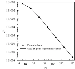
Three complete tests are compared as follows. The first one is a Dirichlet problem on an ellipse x2+ 16y2= 1 with a given boundary condition φ=sin(3x)cosh(3y). Isoparametric quadratic elements are distributed on the boundary, and the 16-point standard Gaussian quadrature is used for non-singular integrals. On singular elements, two different schemes described previously are tested and compared. The first one is the used logarithmic Gaussian quadrature method with 16-point, and the second one is the present subtracting and adding-back technique. Figure 1 shows the root mean square errors of the numerical results of the two different approaches for the singular integration. The present scheme only uses 16-point Gaussian quadrature and performs as well as the traditional logarithmic Gaussian quadrature scheme.

The next example is a mixed boundary condition problem on the same ellipse. The exact solution of this case is still φ=sin(3x)cosh(3y). A part of the boundary is assigned with the velocity potential when 0≤θ ≤π, while the other part takes the normal derivative when π ≤θ ≤2π . Figure 2 and 3 both indicate that the two schemes mentioned previously provide the same accuracy on the solutions of potential and its normal derivative part. Considering these numerical results and calculating procedures, obviously, the present scheme is superior to the traditional logarithmic Gaussian quadrature scheme.

In the last figure, only the present method is tested for the Dirichlet problem with different orders of Gaussian quadrature. The accuracy of results from the two-point Gaussian quadrature is clearly not enough. When four-point or higher formula is used, these error curves indicate the results are convergent when the number of elements

7 -10 20 50 100 200 500 6 1E-006 1E-005 1E-004 1E-003 1E-002 1E-001 1E+000 E2 Present scheme

Used 16-point logarithmic scheme

increases.

2.Conclusions

This study provides an alternative scheme to handle the singular integrals for the 2-D BEM. According to the numerical examples, the present method gives a simple and efficient approach for solving such singular integrals. If the number of elements is not very large, a four-point Gaussian quadrature formula is already good enough for high-order boundary elements.

五、參考文獻

1. Brebbia CA, Dominguez J. Boundary Elements. McGraw-Hill, New York, 1992. 2. Becker AA. The Boundary Element Method in Engineering. McGraw-Hill, New

York, 1992.

3. Kantorovich LV, Krylov VI. Approximate Methods for Higher Analysis. Interscience, 1958.

4. Hwang WS, Hung LP, Ko CH. Nonsingular boundary integral formulations for plane interior potential problems. International Journal for Numerical Methods in Engineering 2002; 53: pp.1751-1762.

5. Abramowitz M, Stegun IA. Handbook of Mathematical Functions. Dover, New York, 1972.

六、成果自評

本研究內容與原計畫相符、並達成預期目標、研究成果兼具學術及應用價 值、適合在學術期刊發表。

附 圖

Figur e 2. Root-mean-squar e er r or s of φ via number of total nodes on an ellipse (a=1,b=1/4) with a mixed boundar y condition φ= sin3xcosh3y when 0 ≤θ≤ π.

10 20 50 100 200 500 6 N 1E-008 1E-007 1E-006 1E-005 1E-004 1E-003 1E-002 1E-001 E2 Present scheme

Used 16-point logarithmic scheme

Figur e 1. Root-mean-squar e er r or s of ∂φ/∂n via number of total nodes on an ellipse (a=1, b=1/4) with the Dir ichlet boundar y condition φ= sin3xcosh3y.

10 20 50 100 200 500 6 N 1E-007 1E-006 1E-005 1E-004 1E-003 1E-002 1E-001 1E+000 E2 Present scheme

Used 16-point logarithmic scheme

10 20 50 100 200 500 6 N 1E-006 1E-005 1E-004 1E-003 1E-002 1E-001 1E+000 1E+001 E2 2-point formula 4-point formula 8-point formula 16-point formula Figur e 3. Root-mean-squar e er r or s of ∂φ/∂n Figur e 6. Root-mean-squar e er r or s of

∂φ/∂n via number of total nodes on an ellipse (a=1,b=1/4) with a mixed boundar y condition φ = sin3xcosh3y

Figur e 4. Root-mean-squar e er r or s of ∂φ/∂n via number of total nodes on an ellipse (a=1, b=1/4) with the Dir ichlet boundar y condition φ= sin3xcosh3y for differ ent or der s of Gaussian quadr atur e for mulas.