先前損失與後續交易行為: 以臺灣期貨市場為例 - 政大學術集成

全文

(1)國立政治大學財務管理研究所碩士論文. 政治大 Prior Losses and 立 subsequent trading behavior of. ‧ 國. 學. different types of traders: Evidence from the. ‧. Taiwan Futures Exchange. n. er. io. sit. y. Nat. al. Ch. engchi. i n U. v. 指導教授：周冠男博士研究生：李家齊撰. 中華民國一百零二年一月.

(2) Abstract Using a dataset from TAIFEX, Taiwan Futures Exchange, we conduct an account-level analysis of the relation between prior loss consequences and subsequent trading behaviors. We apply two proxy variables of trading activities into our analysis, which are trade size and number of trades. We find that the degree of prior losses has a great effect upon trade size and trading number on the next trading day. This finding proves to the evidence that hedonic editing hypothesis sometimes fails and there are. 政治大 results show that individual investors exhibit the strongest bias while other trader 立. some limitations for it. We further examine for different trader types and the empirical. types do uncertainly. We also find the behavioral bias is a persistent phenomenon for. ‧ 國. 學. individual investors. Overall, our study suggests that prior loss degree has a. Nat. n. al. er. io. sit. y. ‧. significant influence on investors’ following trading behaviors.. Ch. engchi. i n U. v.

(3) CONTENTS List of Figures ........................................................................................................ III List of Tables ..........................................................................................................IV 1. Introduction .......................................................................................................... 1 1.1 Motivation .......................................................................................................... 1. 政治大 Outline ................................................................................................................ 2 立. 1.2 Objectives ........................................................................................................... 2 1.3. ‧ 國. 學. 2. Literature Review ............................................................................................... 4 2.1 Prospect Theory .................................................................................................. 4. ‧. 2.2 Mental Accounting ............................................................................................. 6. y. Nat. er. io. sit. 2.3 Hedonic Editing .................................................................................................. 6 2.4 The Failure of Hedonic Editing－Quasi-Hedonic Editing ............................... 10. al. n. v i n Ch Trader Types ..................................................................................................... 11 engchi U. 2.5. 3. Data and Methodology .................................................................................... 12 3.1 Data Description ............................................................................................... 12 3.2 Research Methodology and Hypotheses ........................................................... 13 4. Empirical Results .............................................................................................. 16 4.1 All Investors by Trade Size and Number of Trades ......................................... 16 4.2 Trader Types by Trade Size and Number of Trades......................................... 19 4.3 Robustness checks ............................................................................................ 25 I.

(4) 5. Conclusion ........................................................................................................... 31. References ................................................................................................................ 32. 立. 政治大. ‧. ‧ 國. 學. n. er. io. sit. y. Nat. al. Ch. engchi. II. i n U. v.

(5) List of Figures Figure 1 Prospect Theory－Value Function.............................................................. 5 Figure 2 Prospect Theory－Weighting Function ...................................................... 5 Figure 3 Hedonic Editing－Segregate Gains ............................................................. 8 Figure 4 Hedonic Editing－Integrate Losses ............................................................ 8 Figure 5 Hedonic Editing－Cancel Small Losses from Larger Gains .................... 9 Figure 6 Hedonic Editing－Segregate Small Gains from Larger Losses ............... 9. 立. 政治大. ‧. ‧ 國. 學. n. er. io. sit. y. Nat. al. Ch. engchi. III. i n U. v.

(6) List of Tables Table 1 The Definition of Loss Sizes by Absolute Return and Return Distribution ..................... 15 Table 2 The Characteristics of Three Sample Groups .................................................................... 15 Table 3 Trade Size and Number of Trades for All Investors ........................................................... 18 Table 4 Trade Size and Number of Trades for Domestic Institutions ............................................ 22 Table 5 Trade Size and Number of Trades for Foreign Institutions............................................... 23 Table 6 Trade Size and Number of Trades for Individual Investors .............................................. 24 Table 7 Robustness checks for all investors ...................................................................................... 27. 政治大. Table 8 Robustness checks for domestic institutions ....................................................................... 28. 立. Table 9 Robustness checks for foreign institutions .......................................................................... 29. ‧ 國. 學. Table 10 Robustness checks for individual investors ...................................................................... 30. ‧. n. er. io. sit. y. Nat. al. Ch. engchi. IV. i n U. v.

(7) 1. Introduction 1.1 Motivation Nowadays, academic finance has evolved from efficiency markets to behavioral finance. The research for behaviors is one of the most essential fields in finance, which includes broader concepts such as psychology and sociology. An interesting research links psychology factors and financial behaviors together. Thaler (1985) argues that investors frame multiple outcomes in mental ways that bring the highest perceived value. This process is called ‘’Hedonic Editing’’, which means investors. 政治大. would choose to integrate or segregate multiple outcomes to achieve the maximum. 立. perceived value. The theory suggests four rules: (1) Segregate gains. (2) Integrate. ‧ 國. 學. losses. (3) Cancel small losses from larger gains. (4) Segregate small gains from larger losses.. ‧. Although hedonic editing has been for decades, only few studies have. y. Nat. io. sit. investigated this hypothesis. Thaler and Johnson (1990) conducted a further exam,. n. al. er. which shows that people do not have the same feeling for the same amount of losses. i n U. v. due to the different size of previous losses. For example, the loss of $9 hurt more after. Ch. engchi. a $36 loss than after a $9 loss, while it hurt less after a $1000 loss than a $30 loss. It is the implication that small loss would make investors sensitive to the next loss while big loss numb them to the second one. Besides, Linville and Fischer (1991) found that integration of positive outcomes would contribute to the higher perceived value. However, people prefer to experience two negative events on different days. Thaler and Johnson (1990) then proposed the quasi-hedonic editing hypothesis, which argues that hedonic editing rule is followed partially and fails sometimes. In this article, our ultimate goal is to investigate the failure of hedonic editing. The existing literatures of hedonic editing or quasi-hedonic editing focus on the stock 1.

(8) market. In our study, we use a unique dataset in Taiwan Futures Exchange. We concentrate on loss cases and test whether prior losses have an impact on subsequent trading behaviors for investors. Furthermore, our data allow us to identify trader types, which fall into four categories: domestic institutions, foreign institutions, futures proprietary firms, and individual investors. Some literatures exhibit that individual investors trade with behavior bias rather than other institutional traders. In this paper, we present the relationship of behavior bias and trader types to explore whether trading behaviors differ from each trader type.. 政治大. 立. 1.2 Objectives. ‧ 國. 學. The purpose of this paper is to examine whether investors have dissimilar trading activities when facing the same loss size due to the difference of prior loss degree. If. ‧. it is shown in our research, we can tell that there are some limitations for hedonic. sit. y. Nat. editing since people have different reactions to the same amount of loss.. n. al. er. io. According to our motivation, we derive some expectations as follows. We expect. i n U. v. that investors who suffer greater losses before would be numbed to the second loss so. Ch. engchi. that they do not have conservative attitude and trade more. On the other hand, investors who have smaller losses before become reluctant to endure the next loss, consequently, they are more risk averse and trade less. These expectations correspond with our hypotheses in section 3.2.. 1.3 Outline Here, we provide the reminders for the rest of this paper. Chapter 2 illustrates the relevant literatures, including prospect theory, mental accounting, hedonic editing hypothesis, quasi-hedonic editing hypothesis, and trader type. Chapter 3 describes our 2.

(9) dataset, research methodology, and hypotheses. Our empirical results and robustness checks are presented in chapter 4. Lastly, chapter 5 is the conclusions for this paper.. 立. 政治大. ‧. ‧ 國. 學. n. er. io. sit. y. Nat. al. Ch. engchi. 3. i n U. v.

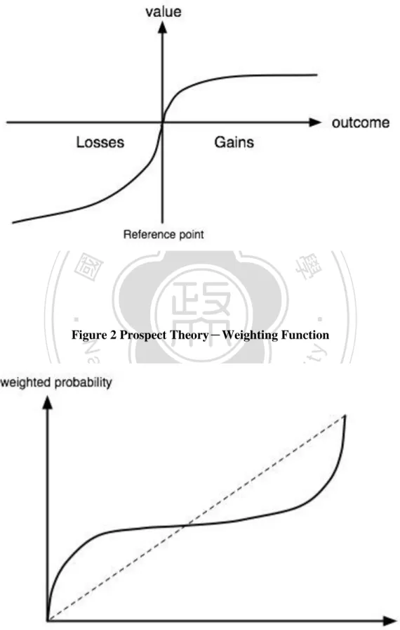
(10) 2. Literature Review We review some financial theories related to human behaviors in this chapter, and the following are brief introductions.. 2.1 Prospect Theory Prospect theory is introduced by Kahneman and Tversky (1979), which describes that investors make decisions based on the perceived value of gains and losses rather. 政治大 theory, which are value function and weighting function. 立. than the final wealth level. There are two important functions derived from prospect. The value function points out the difference between the mental result and. ‧ 國. 學. physical outcome. It suggests that investors define gains and losses from the specific. ‧. reference point but not the final outcome. Figure 1 shows the result. It is changes in. sit. y. Nat. wealth that which determine the value along the vertical axis, rather than terminal. io. er. wealth. The s-shaped value function shows concavity for gains and convexity for losses. The slope of losses is steeper than gains, which can imply that losses have. al. n. v i n more impact to investors than anCequivalent amount ofU h e n g c h i gains (losses hurt more than. gains feel good). It is called ‘’loss aversion’’. The weighting function expresses that investors make decisions based on decision weights rather than objective probability. Investors apparently over-weight when they are facing an event with small probabilities. On the contrary, they tend to under-weight certain outcomes. The function is showed as figure 2.. 4.

(11) Figure 1 Prospect Theory－Value Function. 立. 政治大. ‧. ‧ 國. 學. n. al. er. io. sit. y. Nat. Figure 2 Prospect Theory－Weighting Function. Ch. engchi. 5. i n U. v.

(12) 2.2 Mental Accounting Mental accounting, first named by Richard Thaler (1980), is a general concept on behavioral finance. Based on Thaler’s thesis, it is the set of cognitive operations used by individuals and households to organize, evaluate, and keep track of financial activities. There are three main components of mental accounting. The first one is that how individuals make their decisions and how the subsequent result is affected by prior outcomes. The second component is that how individual separate different accounts and evaluate it. Funds for spending are divided into different consumption. 政治大 Cash inflows are also grouped 立as regular income, windfall, capital gains and so on. In. categories such as daily expenditures, education, entertainment, and luxury goods.. ‧ 國. 學. general, individuals have different preferences and perceived utility on different accounts. The other important component on mental accounting is ‘’choice. ‧. bracketing’’, which is developed by Read, Loewenstein, and Rabin (1998). It. sit. y. Nat. describes that individuals can evaluate accounts based on different time periods, such. n. al. i n U. psychological choice from mental accounting concepts.. Ch. engchi. er. io. as daily, weekly, monthly, yearly and so on. As a result, we can understand the. v. 2.3 Hedonic Editing Hedonic editing hypothesis, as proposed by Richard Thaler (1985), is one of the fundamental theories in behavioral finance. It is based on the assumption that through mental accounting process, investors are inclined to frame multiple outcomes in ways that yield the highest perceived value. Thaler points out that in some cases, the integration of multiple outcomes generate greater perceived value, while in other situations, the highest perceived value is achieved by segregating multiple outcomes. There are four principles derived from hedonic editing as follows. 6.

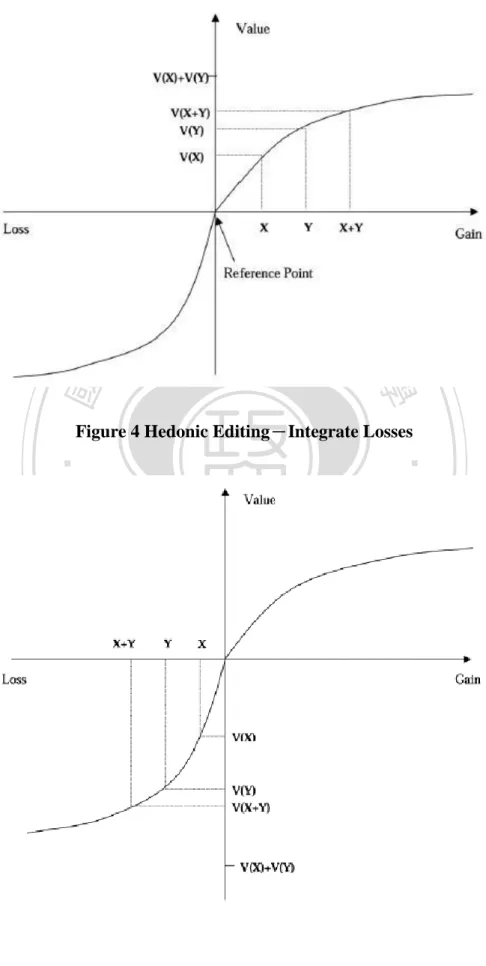
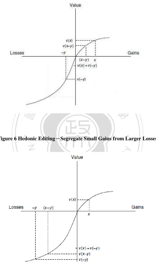
(13) Principle 1: Segregate gains. We learn that the value function is concave in domain of gains from prospect theory, thus, investors are better off valuing gains separately, that is, v(x)+v(y)>v(x+y). Figure 3 shows the result.. Principle 2: Integrate losses. Differed from gains, the shape of value function is convex for losses. We conclude that the higher perceived utility is achieved when investors are integrating. 政治大. losses, that is, v(x)+v(y)<v(x+y). Figure 4 illustrates the result.. 立. ‧ 國. 學. Principle 3: Cancel small losses from larger gains.. Suppose that an investor has two outcomes, which is x and –y, and the absolute. ‧. value of x dominates y (net gain). We know the slope of losses is steeper that gains in. sit. y. Nat. value function. As a result, it is possible that v(x)+v(-y) is negative while v(x+(-y)) is. io. er. positive. Figure 5 shows the result. Therefore, hedonic editing suggests that for the purpose of maximum utility, investors are going to cancel (integrate) small losses. al. n. v i n from larger gains to alleviate theCdiscomfort from getting h e n g c h i U losses.. Principle 4: Segregate small gains from larger losses. Consider if the outcome is x and –y, where the absolute value of y dominates x (net loss). In this case, we cannot ascertain whether integration or segregation is preferred. However, when the absolute value of loss is significantly larger than the absolute value of gain, we can determine that segregating small gains from larger losses results in greater psychological value. Figure 6 illustrates the relationship. When the difference between x and –y is large, segregation is preferred, that is, v(x)+v(-y)>v(x+(-y)). 7.

(14) Figure 3 Hedonic Editing－Segregate Gains. 立. 政治大. ‧ 國. 學. Figure 4 Hedonic Editing－Integrate Losses. ‧. n. er. io. sit. y. Nat. al. Ch. engchi. 8. i n U. v.

(15) Figure 5 Hedonic Editing－Cancel Small Losses from Larger Gains. 立. 政治大. ‧. ‧ 國. 學. Figure 6 Hedonic Editing－Segregate Small Gains from Larger Losses. n. er. io. sit. y. Nat. al. Ch. engchi. 9. i n U. v.

(16) 2.4 The Failure of Hedonic Editing－Quasi-Hedonic Editing According to the literature ‘’Gambling with the House Money and Trying to Break Even: The Effects of Prior Outcomes on Ricky Choice’’ by Richard H. Thaler and Eric J. Johnson (1990), we can know that in some cases investors do not integrate losses. Therefore, Thaler and Johnson replaced original hedonic editing hypothesis with quasi-hedonic editing hypothesis. This finding reveals the hedonic editing rule is followed only part of the time, in particular, it works only for gains but losses. Based on hedonic editing, we know that the integration of losses generates. 政治大 editing suggests something立 different. It points out that prior losses might make. higher perceived utility rather than segregation for investors. However, quasi hedonic. ‧ 國. 學. investors more sensitive toward the next losses. In other words, investors prefer to experience losses one by one (separately) because they become more risk averse after. ‧. bearing an initial loss.. sit. y. Nat. According to quasi hedonic editing theory, Thaler and Johnson conducted further. n. al. er. io. tests on the failure of integrating losses. They found that people had different feeling. i n U. v. for the same amount of losses because of the different sizes of prior losses. In their. Ch. engchi. study, the loss of $9 hurt more after a $36 loss than after a $9 loss, while it hurt less after a $1000 loss than a $30 loss. The inference for this result is that small losses may sensitize people to further losses of same sizes, while big losses may numb people to subsequent small losses. Patricia W. Linville and Gregory W. Fischer (1991) also conducted an experiment to investigate people’s preferences for segregating or combining events. One hundred undergraduates approximately (half men and half women) participated in this study. The research investigated people’s preference for temporally separating or combining events. There are four types of events coinciding with the four situations 10.

(17) of hedonic editing, which are pure gains, pure losses, mixed gains (large gains and small losses), and mixed losses (small gains and large losses). In the pure losses case, Linville and Fischer found that losses will have greater impact when they occur together rather than when they occur separately. Consequently, people prefer to segregate two losses events on different days. The implication referring to this research is called ‘’loss-avoidance hypothesis’’. The larger the losses in case, the stronger the tendency will be, which means that the larger prior losses will leave people more vulnerable to the second losses. However, if. 政治大 loss-buffering which could ease the negative impact. 立. the losses are small enough, people may consider that there are sufficient. ‧ 國. 學. 2.5 Trader Types. ‧. There are many recent literatures indicate the irrational behavior of individual. sit. y. Nat. investors. For example, Barber and Odean (2000) and Barber et al. (2008) exhibit that. n. al. er. io. individual investors suffer economically large loss due to their active trading.. i n U. v. Moreover, Peter R. Locke and Steven C. Mann (2005) found that market professionals. Ch. engchi. have some disciplined strategies to avoid potential behavioral bias. We grab concepts from these studies and apply into our analysis in this paper.. 11.

(18) 3. Data and Methodology 3.1 Data Description We obtain complete trading data for all market traders in the market of TAIEX futures, which is traded on the TAIFEX (Taiwan Future Exchange) for 1,241 trading days from January 2004 to December 2008. The TAIEX futures are future contracts on Taiwan Stock Exchange Index, which is a capitalization weighted index comprised of all common stocks on Taiwan Stock Exchange (TSE). TAIFEX is an order-driven electronic futures market in which there are no market makers, thus futures prices are. 政治大. determined by limit orders of market traders.. 立. On the TAIFEX, the trading hours are 8:45 a.m. to 1:45 p.m., from Monday. ‧ 國. 學. through Friday excluding public holidays. The contract sizes are the TAIEX value X 200 New Taiwan Dollars. The daily price limit is +/- 7% of the settlement price on the. ‧. previous day. Delivery months include the spot month, the next calendar month, and. y. Nat. io. sit. the next three quarterly months. The last trading day is the third Wednesday of the. n. al. er. delivery month for each contract. All contracts are exercised on expiration date. i n U. v. automatically and are settled with cash. We select only nearby contracts in our analysis because of liquidity.. Ch. engchi. The dataset presents the detail information of transactions. It contains the date of transactions, its direction (sell or buy), transaction price, trading quantity, the identity of account and trader types. According to TAIFEX, traders are classified into four types: foreign institutional traders, domestic institutional traders, futures proprietary firms, and individual traders. Because of the identifiable information, we are able to determine the trading activities of different trader types.. 12.

(19) 3.2 Research Methodology and Hypotheses Originally, hedonic editing hypothesis suggests that investors better off combining losses mentally to maximize the value. However, according to quasi-hedonic editing hypothesis and loss-avoidance hypothesis, investors may fail to integrate losses because they become more loss averse after experiencing a previous loss and this inclination is stronger within big losses scenarios. In this paper, we focus on pure losses case. We know that the size of prior losses is an essential cause for subsequent trading activities. Therefore, we consider that. 政治大 risk averse and trade more.立 On the other hand, smaller loss sensitizes investors to the bigger loss makes investors insensitive toward an additional loss so that they are less. ‧ 國. 學. next loss, which is the reason why they are more risk averse and trade less. To examine the limit of hedonic editing, we test whether the subsequent trading activities. ‧. is affected by prior loss results.. sit. y. Nat. First, we grab the trading data of two serial losses from dataset. We regard two. n. al. er. io. serial losses as a reference day. Secondly, we follow Yu-Jane Liu, Chih-Ling Tsai,. i n U. v. Ming-Chun Wang and Ning Zhu (2010) to compute the average of trade size and the. Ch. engchi. number of trades respectively on the following 5 days. Trade size is the total quantity of transacted contracts and the number of trades is the trading frequency in the same day, which can be considered as proxy variables for trading activities. Following, we divide our data by the size of losses. There are two methods we define loss size. One is absolute return, by which we regard less than -10% in return as big loss, falling in -3% to -10% as medium loss, and greater than -3% as small loss. The other is return distribution, by which we consider the return on each trading account to be normal distribution and independent, because we think everyone has different mental editing rules. We define loss size by return distribution in each 13.

(20) trading account. We view the top thirty percent of loss degree as big loss, the intermediate forty percent as medium loss, and the bottom thirty percent as small loss. Table 1 summarizes the definition of loss sizes. Lastly, we comply with the big-, medium-, and small- loss rules to form three sample groups. They have the same size of subsequent loss, while the prior loss size is greatest in group 1 and smallest in group 3. The two serial losses are independent and there are 30 data at least in each sample group. Table 2 presents the characteristics for each group. Investors in group 1 are supposed to be more risk seeking and trade more. 政治大 losses result in sensitizing investors in group 3 so that they become more risk averse 立 afterward because they are numbed by greater prior losses. However, smaller prior. and trade less. Investors in group 2 have middle risk attitude toward subsequent. ‧ 國. 學. trading activities.. ‧. We test the difference of trade size and the number of trades on the following 5. sit. y. Nat. days between three groups. The significant level is 5%. After that, we further examine. io. above, we derive two hypotheses in this paper.. n. al. Ch. engchi. er. whether the result is influenced by trader types. Based on the literature we mentioned. i n U. v. Hypothesis 1: Trade size in group 1 is greater than group 2 and trade size in group 2 is greater than group 3 on the following 5 days of the reference day.. Hypothesis 2: Number of trades in group 1 is greater than group 2 and number of trades in group 2 is greater than group 3 on the following 5 days of the reference day.. 14.

(21) Table 1 The definition of loss sizes by absolute return and return distribution. By absolute return, big loss is defined when the loss is more than 10% while small loss is smaller than 10%. Medium loss is between big loss and small loss. By return distribution, we consider the return on. each day as a normal distribution. The loss which lies on the top of 30% is called big loss and which on the bottom of 30% is small loss. Medium loss is intermediate.. absolute return. return distribution. Big loss. < -10%. Top 30% of loss degree. Medium loss. Between -3% and -10%. Intermediate 40% of loss degree. Small loss. > -3%. Bottom 30% of loss degree. 立. ‧ 國. 學. Table 2. 政治大. The characteristics of three sample groups. In this table, we follow the definition of loss size to form three sample groups. All these three groups are assumed to have the equivalent size of. ‧. subsequent loss. However, the prior loss of group 1 is the biggest, next is group 2, and group 3 has the smallest prior loss.. n. Group 3. al. sit. Subsequent loss. er. io Group 2. y. Nat Group 1. Prior loss. Ch. Big. eMedium ngchi Small. 15. i n U. v. Small Small Small.

(22) 4. Empirical Results We present our empirical results in this chapter. By the methodology we described above, we apply two proxy variables of trading activities respectively in our hypothesis 1 and 2. We compare the trading activities between the three groups to figure out if prior loss degree has impact on subsequent trading behaviors. Then, we test whether trader type is an essential factor of subsequent trading behaviors. Finally, we do some robustness checks by dividing our sample into two periods to confirm our empirical results is objective.. 政治大 results for all investors, section 立 4.2 for different trader types, and in section 4.3, we. As above, we follow two methods to define loss sizes. Section 4.1 shows statistic. ‧. ‧ 國. 學. provide results for robustness checks.. 4.1 All Investors by Trade Size and Number of Trades. sit. y. Nat. io. er. From the statistic summary in Table 3, we can grab some information for all investors. As we mentioned above, there are two methods which we use to define big-,. al. n. v i n C hmethods are absolute medium-, and small- loss. The two return and return distribution. engchi U Thus, we provide the results by two methods separately. Panel A is for absolute return. method and panel B for return distribution method. Both of them show the average trade size and number of trades on the following 5 days for each group. In sum, we can obviously see the average of trade size and trading frequency decrease from group 1 through group 3. They are the biggest in group 1, followed by group 2, and the smallest in group 3. Then, we analyze the trading data and compare the difference of trading activities for three groups by T-test with significant level of 5%. We examine the mean difference between group 1-2 and group 2-3 respectively. Almost all P-value are 16.

(23) under 0.05, which show the difference is strongly significant. The results support our two hypotheses. Investors tend to trade more when they are numbed to the next loss by greater prior losses while they become conservative toward trading because previous smaller loss makes them sensitive to the second loss. In other words, investors are not more likely to have similar risk attitudes when they suffer different loss degree previously.. 立. 政治大. ‧. ‧ 國. 學. n. er. io. sit. y. Nat. al. Ch. engchi. 17. i n U. v.

(24) Table 3 Trade size and number of trades for all investors. In this table, we categorize all investors into three groups by the method mentioned in table 1 and table 2, and then compare mean difference of trading activities (trade size and number of trade) between three groups. We examine group 1 -2 and group 2-3 separately by T-test. The significant level is 5%.. Trade Size. Number of Trades N. Mean. St. Dev.. Mean. St. Dev.. Group 1. 108.5. 301.6. 47.2380. 116.0. 12,510. Group 2. 31.0027. 37.2710. 70,949. 23.8595. 535,049. Panel A: by absolute return. 立. and Group 2 (P-value). (<0.0001). (<0.0001). 16.2888. 7.5463. (<0.0001). (<0.0001). io. sit. y. Nat. and Group 3 (P-value). 28.3417. Panel B: by return distribution. al. n. Group 1. Ch. 86.0710. 398.7. Group 2. 73.5776. 357.5. Group 3. 68.9199. 352.8. engchi. iv n U41.0652. 146.8. 12,574. 36.3335. 135.7. 27,645. 33.8544. 138.3. 28,072. Difference between Group 1. 12.4934. 4.7317. and Group 2 (P-value). (0.0026). (0.0022). 4.6577. 2.4791. (0.1217). (0.0327). Difference between Group 2 and Group 3 (P-value)). ‧. Difference between Group 2. 77.4989. 學. ‧ 國. Difference between Group 1. er. Group 3. 82.6827 18.8962 政治大 14.7139 39.8687 11.3499. 18.

(25) 4.2 Trader Types by Trade Size and Number of Trades We further examine whether trader type would affect the trading activities. We also use two proxy variables of trading activities, trade size and number of trades, to discuss the behavior of different types of investors. Based on the literature above, we found that professional investors eliminate behavior bias by their well-disciplined trading strategy. Furthermore, sophistication and trading experiences also help investors to reduce behavior bias resulted from mental ill.. 政治大 only three types of investor立 we include here, which are domestic institutions, foreign In this section, we test our hypotheses based on different trader types. There are. ‧ 國. 學. institutions, and individual investors. Future proprietary firms are ignored in our study because we do not have sufficient data (less than 30) for this trader type.. ‧. Section 4.2.1 is the results for domestic institutions, 4.2.2 for foreign institutions,. sit. n. al. er. io. different trader types.. y. Nat. 4.2.3 for individual investors, and in 4.2.4 we summarize the statistical results for. Ch. i. e. i n U. v. n g Size c h and Number of Trades 4.2.1 Domestic Institutions by Trade For domestic institutions, we provide the results in Table 4. Panel A and panel B is based on absolute return and return distribution respectively. Let’s take a look at these statistical summaries first. No matter which method we use, it is obvious that trading activities of group 1 are the greatest, followed by group 2, and group 3 is smallest on the following 5 days. Next step, we check if the difference is significant in statistic by T-test. By absolute return, we can see the difference of trading size and trading times between group 1-2 and group 2-3 are big enough so that all the P-value are under 0.0001, 19.

(26) which is extremely significant outcome. Thus, we can tell that behaviors of domestic institutions follow our hypothesis according to this method. However, it is not the case for return distribution method because all of the results are not significantly different, which is showed by P-value greater than 5%. Hence, we conclude that the behavior of domestic institutions is not accordant with our hypothesis on return distribution method.. 4.2.2 Foreign Institutions by Trade Size and Number of Trades. 政治大 follow two sampling methods, which show in panel A and panel B respectively, to 立 We present the statistic results for foreign institutions in Table 5. Again, we. develop difference test for our hypotheses.. ‧ 國. 學. Based on absolute return, trade size and trading frequency of group 1 are the. ‧. greatest. The difference between group1-2 is significant since P-value is under 0.0001.. y. Nat. However, it does not follow our expectation completely because the difference. er. io. sit. between group 2-3 (group 2 – group 3) is negative, which means that trade size and trading times of group 2 are not greater than group 3. It is in opposition to our. n. al. hypothesis.. Ch. engchi. i n U. v. After that, we move to return distribution method. Although it is consistent with our expectation that the mean of trade size and trading frequency decline from group 1 through group 3, the results of T-test show that only the difference between group 2-3 but group 1-2 is significant in statistic. In sum, for foreign institutions, part of result follows our hypotheses while part of it does not.. 4.2.3 Individual Investors by Trade Size and Number of Trades Lastly, we go on individual investors. We provide the results in Table 6. In panel A and panel B, trade size and number of trades in group 1 is more than group 2 and 20.

(27) group 2 is more than group 3. It seems to support our expectation. To verify whether the difference is significant, we do T-test between group 1-2 and group 2-3 again. All P-value are less than significance level of 5%, which indicates significant difference on trading behaviors between three groups. It is accordant with both our hypothesis 1 and hypothesis 2. Owing to the results, we can tell obviously that individual investors seem to trade with behavior bias because the results of T-test are all significant strongly (almost all P-value are under 0.0001). To conclude, the trading behaviors of individual investors follow our hypotheses.. 立. 政治大. ‧ 國. 學. 4.2.4 Summary for Different Types of Trader. In section 4.2, in order to explore the influence of trader types on trading. ‧. activities, we perform statistic data of domestic institutions, foreign institutions, and. sit. y. Nat. individual investors separately.. io. er. We observe that there are different results for three types of traders. Apparently, individual investors are affected by prior loss degree while other trader types are not.. al. n. v i n C hproxy variable or U It is proved by that no matter which which sampling method we engchi. apply to statistical analysis, P-value of mean difference for individual investors are always under 0.0001 (see Table 6). Nevertheless, it is not the same case for domestic institutions and foreign institutions. Part of results are similar to our expectations, part of them are not because the gap of difference between three groups is not sufficient. Therefore, we illustrate that the trading behaviors of individual investors support our hypotheses while other trader types do uncertainly.. 21.

(28) Table 4 Trade size and number of trades for domestic institutions. In this table, we categorize domestic institutions into three groups by the method mentioned in table 1 and table 2, and then compare mean difference of trading activities (trade size and number of trade) between three groups. We examine group 1 -2 and group 2-3 separately by T-test. The significant level is 5%.. Trade Size. Number of Trades N. Mean. St. Dev.. Mean. St. Dev.. Group 1. 159.9. 224.9. 60.8143. 79.6168. 350. Group 2. 73.1683. 52.2327. 505. 35.8395. 1,822. Panel A: by absolute return. 治 34.0218 政 130.4 大. 立 39.6509. and Group 2 (P-value). Nat. 26.7925 (<0.0001). 33.5174 (<0.0001). 12.5871 (<0.0001). n. al. er. io. sit. and Group 3 (P-value). 86.7403 (<0.0001). ‧. Difference between Group 2. Panel B: by return distribution Group 1. 21.4347. y. Difference between Group 1. 79.5173. 學. ‧ 國. Group 3. Ch. e n g353.0 chi. 225.2. i n U. v. 83.3929. 118.0. 168. Group 2. 184.7. 258.8. 76.0492. 98.3702. 386. Group 3. 160.7. 305.6. 64.9080. 105.2. 489. Difference between Group 1 and Group 2 (P-value) Difference between Group 2 and Group 3 (P-value). 40.5604 (0.1813). 7.3436 (0.4804). 23.9541 (0.2099). 11.1412 (0.1098). 22.

(29) Table 5 Trade size and number of trades for foreign institutions. In this table, we categorize foreign institutions into three groups by the method mentioned in table 1 and table 2, and then compare mean difference of trading activities (trade size and number of trade) between three groups. We examine group 1 -2 and group 2-3 separately by T-test. The significant level is 5%.. Trade Size. Number of Trades N. Mean. St. Dev.. Mean. St. Dev.. Group 1. 910.4. 1078.4. 367.1. 527.7. 173. Group 2. 325.6. 196.6. 84. 749.6. 102. Panel A: by absolute return. 立. and Group 2 (P-value). Nat. 584.8 (<0.0001). 237.1 (<0.0001). -97.4104 (0.4914). -69.9538 (0.3671). n. al. er. io. sit. and Group 3 (P-value). Panel B: by return distribution Group 1. 199.9. ‧. Difference between Group 2. 1324.1. y. Difference between Group 1. 423.0. 學. ‧ 國. Group 3. 治 129.9 政 479.9 大. Ch. e n g1700.2 chi. 1528.3. i n U. v. 648.8. 836.8. 152. Group 2. 1493.6. 2019.3. 592.3. 799.9. 372. Group 3. 1192.8. 1805.0. 468.2. 733.7. 507. Difference between Group 1 and Group 2 (P-value) Difference between Group 2 and Group 3 (P-value). 34.7062 (0.8413). 56.5342 (0.4692). 300.8 (0.0228). 124.1 (0.0173). 23.

(30) Table 6 Trade size and number of trades for individual investors. In this table, we categorize individual investors into three groups by the method mentioned in table 1 and table 2, and then compare mean difference of trading activities (trade size and number of trade) between three groups. We examine group 1 -2 and group 2-3 separately by T-test. The significant level is 5%.. Trade Size. Number of Trades N. Mean. St. Dev.. Mean. St. Dev.. Group 1. 95.4270. 259.3. 42.2257. 91.4051. 11,987. Group 2. 30.3483. 36.3211. 70,360. 21.2920. 533,123. Panel A: by absolute return. 治 18.6551 政 79.8958 大. 立 14.5503. io. (<0.0001). 15.7980. 7.3758. (<0.0001). (<0.0001). n. al. (<0.0001). y. Nat. and Group 3 (P-value). 23.5706. Panel B: by return distribution. Ch. e n g315.2 chi. Group 1. 66.2731. Group 2. 52.3353. Group 3. 46.2139. Difference between Group 1 and Group 2 (P-value) Difference between Group 2 and Group 3 (P-value). ‧. Difference between Group 2. 65.0787. sit. and Group 2 (P-value). 11.2793. er. Difference between Group 1. 34.7477. 學. ‧ 國. Group 3. i n U. v. 32.9459. 92.8812. 12,254. 213.7. 28.0709. 74.7592. 26,887. 205.4. 25.1586. 77.1963. 27,075. 13.9378. 4.8750. (<0.0001). (<0.0001). 6.1214. 2.9124. (0.0007). (<0.0001). 24.

(31) 4.3 Robustness checks 4.3.1 The Analysis of Robustness for all investors From this section, we start to do some robustness analyses in order to check the objectivity of empirical results above. We divide our data into two samples from the middle of time. In Table 7, panel A involves the fore half of sample periods, from January 2004 to June 2006, with 620 trading days while panel B includes the remaining periods, from July 2006 to December 2008, with 621 trading days. Here, three groups are sampled by absolute return method and trading activities are the. 政治大 We can see that no matter 立 which sample period is, the results are coherent with. average of trade size and trading numbers on following 5 days of reference day.. ‧ 國. 學. our expectations. Investors in group 1 trade more rather than in group 2 and group 3 due to their risk-seeking attitude resulted from loss numbness. On the other hand,. ‧. investors in group 3 are the most conservative toward making trades since they are. sit. y. Nat. sensitive to the next loss. All P-value are under 0.0001 which indicates the. n. al. er. io. significance in statistic. According to this robustness analysis, we verify the empirical. i n U. v. results we provide in section 4 are unbiased. The degree of prior loss plays an. Ch. engchi. important role in making subsequent trades for all investors.. 4.3.2 The Analysis of Robustness by trader types We further sort data by trader types to develop robustness test, which provides clarification that whether prior loss degree have an impact on following trading activities for each trader type. Trading data of each trader types was also split into samples by two time periods, the earlier 2.5 years and another 2.5 years afterward, for 620 and 621 trading day respectively. We follow absolute return method again and the results of robustness checks for three different trader types are as follows. 25.

(32) For domestic institutions, we provide the result in Table 8. Panel A is the trading data on previous 2.5 years and panel B shows it for the remaining 2.5 years. On the first 2.5 years, the difference of mean between three groups is not significant because P-value is almost higher than 5%. On the back 2.5 years, the average on trade size and trading numbers of group 1 are greater than group 2, and P-value is under 0.0001 showing the difference between group 1-2 is significant. However, the trading activities of group2 do not dominate over group 3 in this time period, which is against our expectations. Overall, it is not clear that the subsequent trading activities of. 政治大 For foreign institutions, we can grab some information from Table 9, which 立. domestic institutions are influenced by previous loss degree.. shows the data on the prior and the back 2.5 years in panel A and panel B respectively.. ‧ 國. 學. To sum up the analysis of robustness, we can tell that foreign institutions trade with. ‧. behavior bias since all P-value are much smaller than 5%. It is evident that prior loss. sit. y. Nat. degree is an essential concern toward trading for foreign institutions.. io. er. Finally, we discuss individual investors in Table 10. As the same format we provide above, panel A and panel B present trading information of individual. al. n. v i n C hthe back 2.5 years. U investors on the fore 2.5 years and The statistical results support engchi our hypotheses because all P-value is under 0.0001, which is an extremely small. number showing the difference of trading activities within three groups is strongly significant. Combining this robustness analysis with our empirical results in section 4.2.3, we draw conclusion that there are irrational behaviors among individual investors and the evidence is obviously objective. That is, the degree of previous loss has a great effect upon the next trading actions for individual investors.. 26.

(33) Table 7 Robustness checks for all investors. In this table, we check the robustness of our results above. We divide all investors to two samples by the middle of year. In robustness analysis here, we sample the data by absolute return only. We examine the difference between group 1-2 and group 2-3 on both the first and the second period by T-test with 5% significant level. Panel A presents the analysis of the first 2.5 years (from January 2004 to June 2006) while panel B shows the remaining 2.5 years (from July 2006 to December 2008).. Trade Size. Number of Trades N. Mean. St. Dev.. Mean. St. Dev.. Panel A: trading activities on the fore 2.5 years. 治 39.0888 政 323.5 大. Group 1. 100.2. 96.2409. 5,427. 62.8730. 14.0544. 26.8915. 30,981. Group 3. 10.6438. 24.9345. 8.0119. 12.9770. 259,214. io. and Group 3 (P-value). (<0.0001). 13.5502. 6.0425. (<0.0001). (<0.0001). n. al. (<0.0001). y. Nat. Difference between Group 2. 25.0344. sit. and Group 2 (P-value). 76.0194. er. Difference between Group 1. ‧. ‧ 國. 立 24.1940. 學. Group 2. Ch. engchi. Panel B: trading activities on the back 2.5 years. i n U. v. Group 1. 114.9. 283.6. 53.4819. 128.8. 7,083. Group 2. 36.2805. 94.9097. 22.6493. 43.2797. 39,968. Group 3. 18.5388. 49.6869. 14.4867. 30.4251. 275,835. Difference between Group 1 and Group 2 (P-value) Difference between Group 2 and Group 3 (P-value). 78.5716. 30.8325. (<0.0001). (<0.0001). 17.7417. 8.1627. (<0.0001). (<0.0001). 27.

(34) Table 8 Robustness checks for domestic institutions. In this table, we check the robustness for domestic institutions. We divide domestic institutions to two samples by the middle of year. In robustness analysis here, we sample the data by absolute return only. We examine the difference between group 1-2 and group 2-3 on both the first and the second period by T-test with 5% significant level. Panel A presents the analysis of the first 2.5 years (from January 2004 to June 2006) while panel B shows the remaining 2.5 years (from July 2006 to December 2008).. Trade Size. Number of Trades N. Mean. St. Dev.. Mean. St. Dev.. 政治大 845.2 845.3 274.2. 252.1. 57. 479.8. 382.3. 222.1. 306.0. 18. 421.7. 445.5. 176.1. 190.5. 13. Panel A: trading activities on the fore 2.5 years. 立. Group 1. Group 3. 52.1345. and Group 2 (P-value). (0.0135). (0.4702). Difference between Group 2. 58.1410. 46.0342. sit. er. io. (0.6359) a l (0.6994) v i n Ch engchi U. n. and Group 3 (P-value). y. Nat. 365.3. ‧. Difference between Group 1. 學. ‧ 國. Group 2. Panel B: trading activities on the back 2.5 years Group 1. 942.5. 1178.3. 412.7. 615.8. 116. Group 2. 283.6. 497.4. 104.8. 147.9. 66. Group 3. 423.2. 1409.0. 203.4. 799.9. 89. Difference between Group 1 and Group 2 (P-value) Difference between Group 2 and Group 3 (P-value). 658.9. 307.9. (<0.0001). (<0.0001). -139.7. -98.5717. (0.3887). (0.2585) 28.

(35) Table 9 Robustness checks for foreign institutions. In this table, we check the robustness for foreign institutions. We divide foreign institutions to two samples by the middle of year. In robustness analysis here, we sample the data by absolute return only. We examine the difference between group 1-2 and group 2-3 on both the first and the second period by T-test with 5% significant level. Panel A presents the analysis of the first 2.5 years (from January 2004 to June 2006) while panel B shows the remaining 2.5 years (from July 2006 to December 2008).. Trade Size. Number of Trades N. Mean. St. Dev.. Mean. St. Dev.. Panel A: trading activities on the fore 2.5 years. 治 42.1233 政 195.8 大. Group 1. 141.9. Group 3. 35.6890. 119.6. 26.4706. 31.2526. 221. 71.5643. 16.4147. 25.0202. 762. 15.6527. (<0.0001). (0.0005). Difference between Group 2. 30.2567. 10.0559. y. and Group 3 (P-value). (0.0004). (<0.0001). Ch. i n U. and Group 2 (P-value). Nat. io. n. al. sit. 75.9721. er. Difference between Group 1. 146. ‧. ‧ 國. 立 65.9457. 學. Group 2. 46.7663. engchi. Panel B: trading activities on the back 2.5 years. v. Group 1. 172.8. 243.2. 74.1912. 94.3637. 204. Group 2. 78.7887. 138.2. 39.8979. 63.4061. 284. Group 3. 42.4991. 84.6936. 25.0434. 41.5655. 1,060. Difference between Group 1 and Group 2 (P-value) Difference between Group 2 and Group 3 (P-value). 93.9956. 34.2933. (<0.0001). (<0.0001). 36.2897. 14.8545. (<0.0001). (0.0002). 29.

(36) Table 10 Robustness checks for individual investors. In this table, we check the robustness for individual investors. We divide individual investors to two samples by the middle of year. In robustness analysis here, we sample the data by absolute return only. We examine the difference between group 1-2 and group 2-3 on both the first and the second period by T-test with 5% significant level. Panel A presents the analysis of the first 2.5 years (from January 2004 to June 2006) while panel B shows the remaining 2.5 years (from July 2006 to December 2008).. Trade Size. Number of Trades N. Mean. St. Dev.. Mean. St. Dev.. 政治大 90.9194 306.2 36.4382. 90.9365. 5,224. 23.6270. 60.5484. 13.8433. 25.3677. 30,742. 10.5492. 24.2681. 7.9787. 12.7964. 258,439. Panel A: trading activities on the fore 2.5 years. 立. Group 3. (<0.0001). (<0.0001). 13.0778. 5.8646. io. sit. Difference between Group 2. (<0.0001) a l (<0.0001) v i n Ch engchi U. n. and Group 3 (P-value). 22.5948. y. Nat. and Group 2 (P-value). 67.2924. ‧. Difference between Group 1. 學. ‧ 國. Group 2. er. Group 1. Panel B: trading activities on the back 2.5 years Group 1. 98.9089. 216.2. 46.6963. 91.5219. 6,763. Group 2. 35.5638. 91.8134. 22.3889. 42.5636. 39,618. Group 3. 18.3148. 41.9530. 14.3846. 26.5693. 274,684. Difference between Group 1 and Group 2 (P-value) Difference between Group 2 and Group 3 (P-value). 63.3451. 24.3074. (<0.0001). (<0.0001). 17.2490. 8.0042. (<0.0001). (0.0002) 30.

(37) 5. Conclusion Behavioral finance provides another explanations and predictions of people’s decision, which lays emphasis on psychology and social sciences rather than human rationality. One of the substantial theories is hedonic editing, which argues that people would choose to integrate or segregate multiple outcomes to realize the highest perceived value. However, we know that people would not follow this mental framing rule in some cases, in particular, for losses case. Therefore, quasi-hedonic editing has taken place of hedonic editing hypothesis. We focus on losses case in this thesis. The. 政治大 prior loss is, the more willing 立investors would trade. In contrast, investors are more. empirical results show that when facing the equivalent amount of losses, the higher. ‧ 國. 學. unwilling to trade due to the smaller prior loss. It is because investors are sensitized by smaller loss and numbed by greater ones previously. Smaller loss makes investors. ‧. sensitive to the second loss so that they are risk averse and trade less. Comparatively,. sit. y. Nat. investors are insensitive to the next loss due to the numbness by greater loss, as a. n. al. er. io. consequence, they make more trades. It is the evidence for the failure of hedonic. i n U. v. editing hypothesis. Further, we examine whether this behavioral bias is an explanation. Ch. engchi. for each trader types. We categorize our dataset and test three types of trader separately. Generally, individual investors exhibit the strongest significant bias on quasi-hedonic editing while domestic institutions and foreign institutions have no obvious significance on this issue. It follows our predictions that professional trading experience and well-disciplined investment strategy are helpful in alleviating behavioral bias. Compared to other trader types, most individual investors lack training in investment, which is the reason for their irrational trading behaviors. In conclusion, our study proposes an exception for hedonic editing hypothesis and supports quasi-hedonic editing hypothesis. 31.

(38) References 1.. Barber, B. M., and Odean, T., 2000. Trading is hazardous to your wealth: The common stock investment performance of individual investors. Journal of Finance 55, 773-806.. 2.. Barber, B. M., and Odean, T., 2001. Boys will be boys: Gender, overconfidence, and common stock investment. Quarterly Journal of Economics 116, 261-292.. 3.. Barber, B. M., Lee, Y. T., Liu, Y. J., and Odean, T., 2008. Just how much do individual investors lose by trading. Review of Financial Studies 22, 609-632.. 政治大 the disposition effect. 立 Working paper, National Chengchi University.. Chou, R. K., Wang, Y. Y., and Yan, X, 2013. Trader types and consequences of. 5.. Kahneman, D., and Tversky, A., 1979. Prospect theory: An analysis of decision. ‧ 國. 學. 4.. under risk. Econometrica 47, 263-291.. ‧. 6.. Linville, P. W., and Fischer, G. W., 1991. Preferences for separating or. y. sit. n. al. er. Locke, P. R., and Mann, S. C., 2005. Professional trader discipline and trade. io. 7.. Nat. combining events. Journal of Personality and Social Psychology 60(1), 5-23.. i n U. v. disposition. Journal of Financial Economics 76, 401-444. 8.. Ch. engchi. Lim, S. S., 2006. Do investors integrate losses and segregate gains? Mental accounting and investor trading decisions. Journal of Business 79, 2539-2574.. 9.. Lehenkari, M., 2009. The hedonic editing hypothesis: evidence from the Finnish stock market. The Journal of Behavioral Finance 10, 9-18.. 10. Liu, Y. J., Tsai, C. L., Wang, M. C., and Zhu, N., 2010. Prior consequences and subsequent risk taking: New field evidence from the Taiwan Futures Exchange. Management Science 56, 606-620. 11. Read, D., Loewenstein, G., and Rabin, M., 1999. Choice Bracketing. Journal of Risk and Uncertainty 19, 171-197. 32.

(39) 12. Shiller, R. J., 2003. From efficient markets theory to behavioral finance. Journal of Economic Perspectives 17, 83-104. 13. Thaler, R. H., 1985. Mental accounting and consumer choice. Marketing Science 4, 199-214. 14. Thaler, R. H., and Johnson E. J., 1990. Gambling with the house money and trying to break even: The effects of prior outcomes on risky choice. Management Science 36, 643-660. 15. Thaler, R. H., 1999. Mental accounting matters. Journal of Behavioral Decision Making 12, 183-206.. 立. 政治大. ‧. ‧ 國. 學. n. er. io. sit. y. Nat. al. Ch. engchi. 33. i n U. v.

(40)