國立交通大學
電子工程學系 電子研究所碩士班
碩 士 論 文
適用於 3GPP-LTE 規格的可重組渦輪解碼器之研究
Research on Reconfigurable Turbo Decoder
for 3GPP-LTE Applications
學生:李永裕
指導教授:張錫嘉 教授
適用於 3GPP-LTE 規格的可重組渦輪解碼器之研究
Research on Reconfigurable Turbo Decoder
for 3GPP-LTE Applications
研 究 生:李永裕
Student:Yung-Yu Lee
指導教授:張錫嘉教授
Advisor:Hsie-Chia Chang
國 立 交 通 大 學
電子工程學系 電子研究所 碩士班
碩 士 論 文
A ThesisSubmitted to Department of Electronics Engineering & Institute Electronics College of Electrical and Computer Engineering
National Chiao Tung University In Partial Fulfillment of the Requirements
for the Degree of Master of Science
in
Electronics Engineering October 2008
適用於 3GPP-LTE 規格的可重組渦輪解碼器之研究
學生:李永裕
指導教授:張錫嘉 教授
國立交通大學
電子工程學系 電子研究所碩士班
摘 要
本論文提出了一個支援全模式且可重組的渦輪解碼器。我們提出的解碼器可 以支援所有定義在 3GPP-LTE 規格裡的編碼長度。而為了提高傳輸速度,遞迴解 碼的平行架構更是受到關注。具有 contention-free 特性的二次多項式交錯器也被 應用在渦輪解碼器的平行架構中。Max-Log MAP 演算法也被採用,可使在極小 的效能損失下有效的減低硬體複雜度。此外,可重組的 1/2/4/8-MAP 解碼器設計 也被提出,此設計可使在解碼過程中,根據所需的效能或傳輸速度,提供一個解 碼器可重組的功能。而依據二次多項式交錯器的特性,一個稱為 residue-only interleaver 的方法可被用來減少記憶體的使用量。 根據在 90nm製程下的實驗結果,在 8 次迴圈的解碼模式下可以達到 130Mb/s 的傳輸速度,晶片面積是 2.10mm2。此外,在 0.9V的供應電壓,277MHz的操作 頻率且編碼長度 6144 下,功率消耗經量測過後為 149.03mW。Research on Reconfigurable Turbo Decoder
for 3GPP-LTE Applications
Student:Yung-Yu
Lee
Advisor:Dr. Hsie-Chia Chang
Department of Electronics Engineering
Institute of Electronics
National Chiao Tung University
Abstract
In this thesis, a fully compliant and reconfigurable turbo decoder is presented to support all block lengths specified in 3GPP-LTE system. The contention-free quadratic permutation polynomial (QPP) interleaver is also introduced for parallel architecture of turbo codes. The parallel processing of iterative decoding is of interest for throughput increasing. The Max-Log MAP algorithm is used to reduce the hardware complexity with the minimized performance loss. Moreover, the reconfigurable 1/2/4/8-MAP decoders is proposed to decode the received codewords based on performance or throughput expected in different conditions. Based on QPP characteristic, the residue-only interleaver is adopted to reduce the memory storage.
After implementation in a 90-nm 1P9M technology, the 130Mb/s data rate with 8 decoding iterations can be achieved in the 2.10 mm2 core area containing 602K gates. According to the post-layout simulation, the power consumption is 149.03mW
Acknowledgement
Firs of all, I would like to express my deepest gratitude to my advisor, Dr. Hsie-Chia Chang, for his enthusiastic guidance and great patience. I learn a lot from his positive attitude in way of research and many other areas. Secondly, I really appreciate Dr. Shyue-Win Wei, Dr. Chun-Hsiung Chuang and Dr. Mao-Ching Chiu for serving as my committees. Heartfelt thanks are also offered to all members in the OCEAN and OASIS group for their constant encouragement and assistance whenever I need.
I would like to show my sincere thanks to my parents for their invaluable care and love. When I was depressed, they comforted and encourage me, and whenever I met difficulty, their heart and mind were always by my side. I also appreciate for their supply to every thing I need without any complaining. Without them, I would not exist in this world. Without them, I would not live to this age. Without them, I would not be here today. Sincerely, it is not enough to give all my appreciation to my dear parents. I would like to attribute all my achievement and honor to them. Thank you mom and dad, I love you forever.
Finally, I appreciate all my true friends for their immediately encouraging when I was down. They let me know that someone other than my parents in this world are caring me, I am not alone to fight. I am willing to share my honor with you guys, thank you every one.
Contents
1 Introduction 1 1.1 Background . . . 1 1.2 Motivation . . . 1 1.3 Thesis Organization . . . 3 2 Turbo Code 4 2.1 Turbo principle . . . 4 2.1.1 Turbo encoding . . . 4 2.1.2 Turbo interleaver . . . 5 2.1.3 Turbo decoding . . . 62.1.4 Error floor effect . . . 7
2.2 Decoding algorithm . . . 8
2.2.1 The MAP algorithm . . . 8
2.2.2 The Log-MAP algorithm . . . 12
2.2.3 The Max-Log-MAP algorithm . . . 14
2.3 Sliding window approach . . . 15
3 Turbo Code in 3GPP-LTE system 17 3.1 Encoding procedure . . . 17
3.2 QPP interleaver . . . 19
3.2.1 Contention-free interleaver . . . 19
3.2.2 Performance comparison . . . 20
3.3 Decoding procedure . . . 21
4 Reconfigurable 3GPP-LTE Turbo Decoder 28
4.1 Architecture overview . . . 29
4.2 MAP decoder . . . 30
4.2.1 Decoding schedule . . . 30
4.2.2 The circuit for LLR calculation . . . 32
4.3 Proposed Turbo decoder design . . . 32
4.3.1 Residue-only interleaver . . . 34
4.3.2 Reconfigurable 1/2/4/8-MAP decoders . . . 36
4.3.3 Throughput consideration . . . 39
5 Implementation Results 43 5.1 Chip characteristic . . . 43
5.2 Comparison . . . 46
6 Conclusion and Discussion 48 6.1 Conclusion . . . 48
6.2 Discussion . . . 48
List of Figures
1.1 Block diagram of digital communication system. . . 2
2.1 Turbo encoder. . . 5
2.2 Turbo encoder for 3GPP2 standard. . . 6
2.3 Trellis termination. . . 7
2.4 Conventional Turbo decoder. . . 7
2.5 A (2,1,2) RSC encoder and its state transition diagram. . . 9
2.6 The decoding trellis diagram of the (2,1,2) RSC encoder. . . 10
2.7 The process diagram of sliding window algorithm. . . 15
3.1 Turbo encoder for 3GPP-LTE. . . 18
3.2 Example of a contention-free permutation. . . 21
3.3 Performance comparison. . . 22
3.4 Comparison of window size. . . 25
3.5 Fixed point comparison. . . 26
3.6 Performance of 3GPP-LTE turbo decoder. . . 27
4.1 Iterative decoding flow of turbo decoder. . . 29
4.2 Block diagram of proposed turbo decoder. . . 30
4.3 Block diagram of MAP decoder. . . 31
4.4 Decoding schedule of MAP decoder. . . 32
4.5 The circuit for LLR unit. . . 33
4.6 Proposed turbo decoder architecture. . . 34
4.7 Example of residue-only interleaver. . . 36
4.9 Short block length 40 of 1/2/4/8-SISO decoders without warm-up free
method. . . 38
4.10 Performance comparison of size 40 of 1/2/4/8 decoders with warm-up free method. . . 39
4.11 Performance comparison of size 6144 of 1/2/4/8 decoders with warm-up free method. . . 40
4.12 Performance of size 40 and 512 under various iterations. . . 41
4.13 Performance of size 2048 and 6144 under various iterations. . . 41
5.1 Layout photo of 3GPP-LTE turbo decoder. . . 46
6.1 Example of multiple codewords store in memories (Length=40). . . 51
6.2 Schedule of decoding 8 codewords. . . 52
6.3 Schedule of decoding 4 codewords. . . 53
6.4 Schedule of decoding 2 codewords. . . 54
A.1 QPP parameters . . . 55
List of Tables
3.1 MAP Decoder Specification . . . 25
3.2 Summary of fixed representation in MAP decoder . . . 26
4.1 Standard specifications for turbo coding . . . 28
4.2 Needed iterations of different size . . . 39
5.1 Efficiency of each SISO decoder with 1/2/4/8-decoders . . . 43
5.2 Throughput summary . . . 44
5.3 3GPP-LTE turbo decoder chip summary . . . 45
5.4 Comparison of different turbo decoders . . . 47
Chapter 1
Introduction
1.1
Background
The fourth-generation (4G) is a term used to describe the next complete evolution in wireless communications. Several communication applications in the future may demand for a higher speed channel coding scheme. The approaching 4G wireless systems are projected to achieve 100 Mbps to 1Gbps data rate by 2010. The high throughput turbo codes are required in many 4G communication systems. The two significant examples are 3GPP Long Term Evolution (LTE) and IEEE 802.16e WiMax. Some 4G systems use different types of turbo coding schemes. That is, binary codes is used in 3GPP-LTE and duo-binary codes is utilized in WiMax. Although the 4G is now still in formative stages. They may become commercially in the following years.
1.2
Motivation
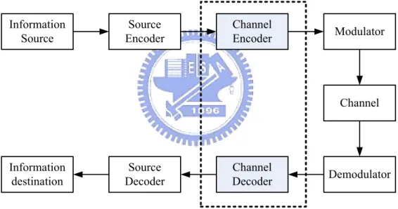
The fundamental block diagram of traditional digital communication system is il-lustrated in Fig. 1.1. The communication system conveys a information source to a destination through a channel. Generally, the system consists of transmitter and receiver via a channel. The transmitter includes source encoder, channel encoder and modulator, is to transform the information into a form that can withstand the effect of noise over the transmission media. Furthermore, the receiver will reverse the signal transformation by demodulator, channel decoder and source decoder. Since the channel impairments such as
noise, interference and distortion may cause the error in the received signal, the channel encoder is incorporated in the system to add certain structural redundancy to the source codeword to minimize the transmission errors. These redundant bits can be used for error detecting and correcting. The channel coding eliminate the effects of noise disturbances and can improve the performance, compared with an uncoded system.
Turbo code is one of the most popular channel coding technique for modern digital communication systems. It is impressive by its excellent error correction ability based on the soft iterative decoding. In the Third Generation Partnership Projects 3GPP and 3GPP2 defined detail standard, they both adopt turbo codes as their channel coding scheme and provide the maximum data rate of about 2 Mb/s and 3 Mb/s, respectively. However, the applications in the future may require higher data rate. Therefore, how to increase the throughput and reduce decoding latency may become obstacles for the turbo code in the hardware implementation.
Information Source Source Encoder Channel Encoder Modulator Information destination Source Decoder Channel Decoder Demodulator Channel
Figure 1.1: Block diagram of digital communication system.
In this thesis, our work is motivated to design a turbo decoder for 3GPP-LTE ap-plications. We attempt to achieve two targets : The first one is to support all block lengths in the standard. The other is to achieve the throughput requirement of 3GPP-LTE specification. Therefore, we employ a contention-free interleaver that fits for parallel decoding architecture to reduce the latency and increase the throughput. Finally, we pro-pose a reconfigurable turbo decoder that fits for whole code lengths and present a practical
hardware architecture for the complete turbo decoder with the modest hardware cost.
1.3
Thesis Organization
This thesis consists of 6 chapters. In chapter 2, the concept of turbo principle and iterative decoding algorithm of turbo codes will be introduced. The turbo codes applied in 3GPP-LTE system, which includes encoding, interleaver and decoding procedure are presented in chapter 3. Furthermore, the simulation analysis and parameter decision are also described. Chapter 4 introduces the design of reconfigurable 3GPP-LTE turbo de-coder, including the hardware architecture and the characteristic of proposed decoder. In chapter 5, the chip implementation result will be shown in detail. Finally, the conclu-sion is given in chapter 6. The parameters used in 3GPP-LTE internal interleaver are illustrated in Appendix A.
Chapter 2
Turbo Code
The parallel concatenated convolutional code (PCCC), named turbo code, was first proposed by C. Berrou, A. Glavieux, and P. Thitimajshima in 1993. It has been proved to have a performance near Shannon limit with simple constituent codes concatenated by an interleaver. Turbo code is adopted in 3GPP, 3GPP2 and WiMAX standards due to its excellent error correction ability. In this chapter, both turbo encoding and turbo decoding methods will be described. The error floor effect in turbo decoding and some decoding techniques will also be interpreted.
2.1
Turbo principle
2.1.1
Turbo encoding
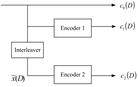
The turbo encoder is composed of two recursive systematic convolutional (RSC) en-coders, which are connected in parallel but separated by an interleaver. The block diagram of the turbo encoder is illustrated in Fig. 2.1. In the first encoder, the information symbols are encoded to the systematic part c0(D) and the parity c1(D); thus, c0(D) = x(D). The
second encoder encodes ˜x(D), the information sequence x(D) after interleaving. However,
the systematic part which is also ˜x(D) will be discarded during transmission because x0
has carried the information sequence. If the code rates of encoder 1 and encoder 2 are R1
and R2 respectively, the overall code rate R in Fig. 2.1 will satisfy
1 R = 1 R1 + 1 R2 − 1. (2.1)
Encoder 1
Encoder 2
Interleaver
( )
D
x
)
(
~ D
x
( )
D
c
0( )
D
c
1( )
D
c
2Figure 2.1: Turbo encoder.
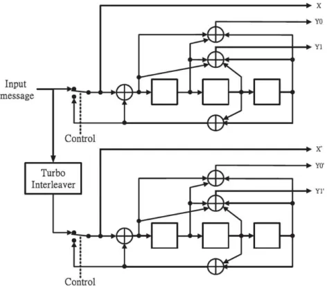
In 3GPP2 standard [1], each input bit is encoded as one systematic bit and two parity-check bits for each RSC encoder. Thus, the code rate of each component encoder is 1/3. In order to increase the code rate of turbo code, the systematic bits of the second RSC encoder are not transmitted. Therefore, the output should be {X, Y0, Y1, Y
′ 0, Y
′
1}, and the
overall code rate is 1/5. It will be shown in Fig. 2.2.
After encoding all information sequence, several tail bits have to be generated to set both component encoders back to zero state. However, it’s impossible for a RSC encoder to return zero state by inserting dummy zeros into the encoder directly. Thus, a solution is provided in Fig. 2.3. While encoding input information, the switch is set to position ”A”. When whole block are encoded, the position of switch is changed to ”B” for three additional cycles. This will force all registers back to zero state.
2.1.2
Turbo interleaver
The interleaver is a critical component for channel coding performance of turbo codes. First of all, a proper coding gain can be achieved with small memory RSC encoders since the interleaver scramble a long block message. Besides, the interleaver de-correlates the input of two RSC encoders so that iterative decoding algorithm can be applied between two component decoders. Theoretically, the block size of interleaver is one of the major factors to lower the upper-bound on bit error probability of the turbo code system. The performance upper-bound of turbo code corresponding to a uniform random interleaver
Figure 2.2: Turbo encoder for 3GPP2 standard.
has been evaluated in [2]. The bit-error-probability upper bound of turbo code is approx-imately proportional to 1/N, where N is the interleaver size. The factor 1/N is also called the interleaver gain.
2.1.3
Turbo decoding
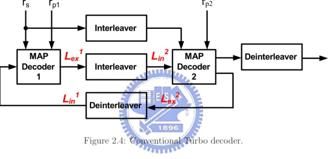
A general idea for iterative turbo decoding is illustrated in Fig. 2.4, where rs is the
received systematic information, rp1 is the received parity information generated by the
first RSC encoder, and rp2 is the received parity information generated by the second
RSC encoder. The iterative turbo decoding consists of two constituent SISO (soft in/soft out) decoders, which are concatenated serially via the interleaver and de-interleaver. An additional interleaver is used to interleave the input systematic information and then provides the interleaved data to the second SISO decoder. During iterative decoding
process, each constituent decoder delivers the extrinsic information Lex which is taken
as a priori information Lin for the other constituent decoder after the interleaver and
de-interleaver process. That is, L1
Figure 2.3: Trellis termination.
increases, better coding gain is expected. However, there is no significant performance improvement if a threshold of the iteration numbers has be reached.
MAP Decoder 1 MAP Decoder 2 Interleaver
r
sr
p1 InterleaverL
ex2 Deinterleaver Deinterleaverr
p2L
ex1L
in2L
in1Figure 2.4: Conventional Turbo decoder.
2.1.4
Error floor effect
Although turbo coding provides an excellent performance, the bit-error-rate (BER) certainly decrease quite slowly at high signal-to-noise ratio (SNR). This phenomenon is due to relative small free distance of turbo codes, and is called an error floor [3]. Consider the relation of minimum free distance and the bit error probability in turbo coding, which can be expressed by Pb ∝ Q Ãr 2df reeR Eb N0 ! , (2.2)
where df ree is the minimum free distance, R is the code rate, and Eb/N0 is the SNR. At
information and parity information can be regarded as highly independent events. How-ever, as the channel provides a reliable transmission, the dependency of the systematic and parity information grows up and the interleaver does little contribution on iterative decoding. To overcome this issue, the interleaver size should be enlarged to lower the error floor.
2.2
Decoding algorithm
The turbo code is composed of two SISO constituent codes that communicate itera-tively through an interleaver. The maximum a posteriori probability (MAP) [4] algorithm and soft-output Viterbi algorithm (SOVA) [5] are commonly employed for the SISO de-coders. Unlike the SOVA which exploits maximum likelihood (ML) algorithm to minimize the word error probability, the MAP algorithm minimizes the symbol (or bit) error prob-ability. In this section, we will focus on introducing the turbo decoding based on MAP algorithm, because it has been proved that the MAP algorithm is the optimal decoding method for turbo codes while comparing with SOVA [6]. Furthermore, the Log MAP and Max-Log MAP algorithms will also be introduced, which reduce the hardware complexity and are widely used for implementation.
2.2.1
The MAP algorithm
The MAP decoding algorithm, termed as BCJR algorithm, is developed by Bahl,
Cocke, Jelinek, and Raviv [4] in 1974. For each transmitted information bit ut, the
MAP algorithm estimates the a posteriori probabilities (APP) based on the received code sequence r over a discrete memoryless channel (DMC). It computes the log-likelihood ratio (LLR)
L(ut) = log
P (ut = +1|r)
P (ut = −1|r)
, (2.3)
for 1 ≤ t ≤ N , where N is the received sequence length, and compares this value to a zero threshold to determine the hard estimate ut as
ut= +1, if L(ˆut) ≥ 0 −1, otherwise (2.4)
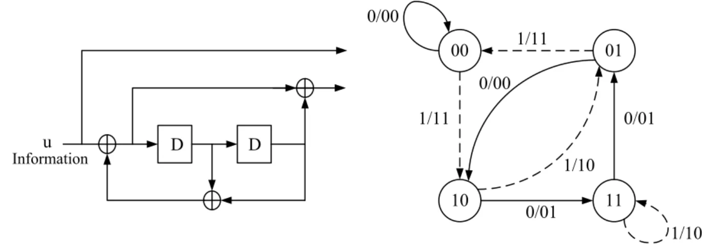
u 00 01 10 11 1/11 1/10 1/10 1/11 0/00 0/00 0/01 0/01 D D Information
Figure 2.5: A (2,1,2) RSC encoder and its state transition diagram.
As an example, a rate 1/2 memory order 2 RSC encoder and its state transition are illustrated in Fig. 2.5. Note that the solid lines represent the state transitions correspond-ing to an information bit ut of −1, while the dotted lines represent the state transitions
corresponding to an information bit utof +1. Its decoding trellis diagram is shown in Fig.
2.6. In Fig. 2.6, the APP’s in (2.3) can be computed by the summation of state transition probabilities. Therefore, the equation can be further expressed as
L(ˆut) = log P (ut = +1|r) P (ut = −1|r) = log P (m′,m)∈B+1 t P (St−1 = m ′, S t= m|r) P (m′,m)∈B−1 t P (St−1 = m ′, S t= m|r) = log P (m′,m)∈B+1t P (St−1 = m ′, S t= m, r) P (m′,m)∈B−1 t P (St−1 = m ′, S t= m, r) , (2.5)
where P (St−1 = m′, St = m, r) represents the joint probability for the existing transition
from St−1 at time t to St at time t + 1. B+1t and B−1t is the sets of (m′, m), denoted the
state transitions which are due to input bit ut = +1 and ut= −1 respectively.
In order to compute joint probability required for calculation of L(ut) in (2.5), we
define the following metrics:
λt(m′, m) = P (St−1 = m′, St= m, r) (2.6)
αt(m) = P {St = m, rt0} (2.7)
βt(m) = P {rN−1t+1 |St= m} (2.8)
Forward Direction for computing
Backward Direction for computing ut = _1 ut = +1
α
β
S
t-1S
t 00 01 10 11Figure 2.6: The decoding trellis diagram of the (2,1,2) RSC encoder.
Since we assume the code sequence after encoding is transmitted through discrete memoryless channel, the joint probability can be expressed as
λt(m′, m) = P (St−1 = m′, St = m, rt−10 , rt, rN−1t+1 ) = P (rN−1t+1 |St−1 = m′, St= m, rt−10 , rt) · P (St= m, rt|St−1 = m′, rt−10 ) · P (St−1 = m′, rt−10 ) = P (rN−1t+1 |St= m) · P (St= m, rt|St−1 = m′) · P (St−1 = m′, rt−10 ). (2.10)
Here rt−10 represents the received code sequence from time instance 0 to t − 1, while rN−1
t+1 is from time instance t + 1 to the end of sequence. Note that the second equation
of (2.10) comes from Bayes’ rule, and the third equation is due to the Markov process in the state transitions. Therefore, compared with the definition of (2.7), (2.8) and (2.9), the joint probability defined in (2.6) can be rewritten as
Now we will derive the equations (2.7), (2.8) and (2.9) as follow: αt(m) = P (St= m, rt−10 ) = X m′∈S P (St−1 = m′, St= m, rt−10 ) = X m′∈S P (St= m, rt−1|St−1 = m′, rt−20 ) · P (St−1 = m′, rt−20 ) = X m′∈S P (St= m, rt−1|St−1 = m′) · P (St−1 = m′, rt−20 ) = X m′∈S αt−1(m′) · γt(m′, m). (2.12) Similarly, we have βt(m) = P (rN−1t+1 |St= m) = X m′∈S P (St+1 = m′, rNt+1−1|St = m) = X m′∈S P (St+1 = m′, rt+1, rN−1t+2 , St= m) / P (St= m) = X m′∈S P (rN−1t+2 |St+1= m′, rt+1, St= m) · P (St+1 = m′, rt+1|St= m) = X m′∈S P (rN−1t+2 |St+1= m′) · P (St+1 = m′, rt+1|St= m) = X m′∈S γt+1(m, m′) · βt+1(m′), (2.13)
where S represent the set of all states. Note that the forward metric α in (2.12) and the backward metric β in (2.13) are computed recursively in opposite direction. If the trellis of encoding diverges from zero state at t = 0 and converges to zero state at t = N − 1, as shown in Fig. 2.6, the following initial conditions are satisfied:
α0(0) = 1, α0(m) = 0 for m 6= 0
βN(0) = 1, βN(m) = 0 for m 6= 0
(2.14)
prob-ability γt(m′, m) can be decomposed as γt(m′, m) = P (St = m, rt|St−1 = m′) = P (St−1 = m ′, S t = m, rt) P (St−1 = m′) = P (St−1 = m ′, S t = m) P (St−1 = m′) · P (St−1 = m ′, S t= m, rt) P (St−1 = m′, St = m) = P (St = m|St−1 = m′) · P (rt|St−1 = m′, St= m) = P (ut) · P (rt|vt), (2.15)
where P (uk) is well-known as a prior probability of uk and vt is the codeword associated
with the transition St−1 = m′ to St= m corresponding to encoder input ut.
As a summary of the MAP algorithm, with computation of γt(m′, m) in (2.15), we can
derive α and β for each state at different time instances. As a result, the joint probability in (2.11) is also available for t = 0, 1, · · · , N − 1. The log-likelihood ratio L(ut) can be
calculated by L(ut) = log P (m′,m)∈B+1 t αt−1(m ′) · γ t(m′, m) · βt(m) P (m′,m)∈B−1 t αt−1(m ′) · γ t(m′, m) · βt(m) . (2.16)
2.2.2
The Log-MAP algorithm
The MAP algorithm requires large memory and a large number of operations involving exponentiations and multiplications. The hardware realization of MAP decoder will be quite complex and difficult. Therefore, the Log-MAP algorithm is proposed to solve this problem. First, we transfer the branch metrics defined in the MAP algorithm to the logarithmic domain; that is
¯
γt(m′, m) = log γt(m′, m). (2.17)
Referring to (2.12) and (2.13), the forward path metric ¯αt can be expressed as
¯ αt(m) = log αt(m) = log X m′∈S eα¯t−1(m′)+¯γt(m′,m) , (2.18)
and the backward path metric ¯βt can be expressed as
¯
βt(m) = log βt(m)
= log X
m′∈S
Note that the initial conditions of path metrics also have changed, since all computations work with the logarithm domain.
¯
α0(0) = 0, α¯0(m) = −∞ for m 6= 0
¯
βN(0) = 0, β¯N(m) = −∞ for m 6= 0
(2.20)
After substituting (2.17), (2.18) and (2.19), the APP information L(ˆut) in (2.16) can be
rewritten as L(ut) = log P (m′,m)∈B+1 t e ¯ αt−1(m′)+¯γt(m′,m)+ ¯βt(m) P (m′,m)∈B−1 t e ¯ αt−1(m′)+¯γt(m′,m)+ ¯βt(m). (2.21) Considering the following Jocobian algorithm [7]
log(eδ1 + eδ2) = max(δ
1, δ2) + log(1 + e−|e
δ2−eδ1|)
= max(δ1, δ2) + fc(|δ2− δ1|),
(2.22)
where fc(·) is a compensation function and thus the performance can be improved. By a
recursive procedure of (2.22), the expression log(eδ1 + eδ2 + · · · + eδn) can be computed exactly, as follows
log(eδ1 + eδ2 + · · · + eδn) = log(∆ + eδn), ∆ = eδ1+ · · · + eδn−1 = eδ = max(log ∆, δn) + fc(|log ∆ − δn|)
= max(δ, δn) + fc(|δ − δn|).
(2.23)
Now we can use (2.22) to represent forward metrics in (2.18) and backward metrics in (2.19) as ¯ αt(m) = max m′∈S ∗{¯α t−1(m′) + ¯γt(m′, m)}, (2.24) and ¯ βt(m) = max m′∈S ∗{¯γ t+1(m, m′) + ¯βt+1(m′)}, (2.25)
where the max∗(·) operation is defined as
max∗(·) = max(δ1, δ2) + fc(|δ2− δ1|). (2.26)
Therefore, the (2.29) can be expressed as L(ˆut) = max (m′,m)∈B+1t ∗{¯α t−1(m′) + ¯γt(m′, m) + ¯βt(m)} − max (m′,m)∈B−1 t ∗{¯α t−1(m′) + ¯γt(m′, m) + ¯βt(m)}. (2.27)
The performance of the Log-MAP algorithm is equivalent to the performance of the MAP algorithm but the complexity has been reduced considerately. However, some dif-ficulty for hardware implementation still exists since computing fc(·) also involves
expo-nentiations and multiplications. For simplified the computation of correction function, it is usually stored in a pre-computed table. This table is only one dimensional due to the
correction only depends on |δ2− δ1|. Thus, the Log-MAP algorithm can be implemented
with max function as well as a lookup table.
2.2.3
The Max-Log-MAP algorithm
In order to further simplify the complexity, another approximation of MAP algorithm termed Max-Log-MAP algorithm is derived. Considering the following approximation formula max function
log(eδ1 + eδ2
+ · · · + eδn
) ≈ max
i∈{1,2,·,n}δi. (2.28)
Note that the term fc(·) is ignored in comparison with (2.23). Then we can simplify the
equation (2.21) as follows: L(ut) = max (m′,m)∈B+1 t {¯αt−1(m′) + ¯γt(m′, m) + ¯βt(m)} − max (m′,m)∈B−1 t {¯αt−1(m′) + ¯γt(m′, m) + ¯βt(m)}. (2.29)
Similarly, the forward recursive and backward recursive metrics in (2.18) and (2.19) can be individually expressed as ¯ αt(m) = max m′∈S{¯αt−1(m ′) + ¯γ t(m′, m)}, (2.30) and ¯ βt(m) = max m′∈S{¯γt+1(m, m ′) + ¯β t+1(m′)}. (2.31)
The computations of ¯α and ¯β are reduced to simple add-compare-select (ACS)
opera-tions, which are equivalent to the path metric updating of Viterbi algorithm. Therefore, compared with the MAP algorithm, the Max-Log-MAP algorithm utilizes additions to replace the multiplications and avoids the complicated exponentiations. However, the performance would degrade because of the information loss in (2.28).
2.3
Sliding window approach
In the conventional MAP-series decoding algorithm(including MAP algorithm, Max-Log MAP algorithm and Max-Log-MAP algorithm), the LLR computation requires the path metric values generated by the forward and backward processes. Furthermore, since the backward recursive computation initials from the end of decoding trellis, as shown in Fig. 2.6, the decoding process can be started after the entire block message to be received. If the sequence length is large, it will lead to long output latency and huge memory requirement for hardware implementation. For example, the maximum block length of 3GPP standard is 5114, which means 5114 LLR values and path metrics should be stored. It is the main disadvantage of turbo code for real applications.
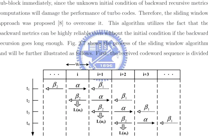
The main problem is that long block length can not be divided into several short sub-block immediately, since the unknown initial condition of backward recursive metrics computations will damage the performance of turbo codes. Therefore, the sliding window approach was proposed [8] to overcome it. This algorithm utilizes the fact that the backward metrics can be highly reliable even without the initial condition if the backward recursion goes long enough. Fig. 2.7 shows the process of the sliding window algorithm and will be further illustrated as follows. First, the received codeword sequence is divided
i i+1 i+2 i+3
L(ut) L(ut) L(ut) t1 t2 t3 t4 W
α
β
1 2β
1β
1β
2β
1β
2β
α
2β
α
α
Figure 2.7: The process diagram of sliding window algorithm.
into several sub-blocks of length of W . W is called the convergence length, which normally is set to be five times the constraint length of component encoder in turbo code to ensure the reliable initialization. In the sliding window approach, the end of sub-block is the initial of next sub-block whether the forward or backward recursive operation. Thus, the
initial metric values are inherited from the last metrics calculated in the previous
sub-block. Note that the dummy backward recursion β1 is employed to establish the initial
condition for the true backward recursion β2. Although the initial condition for the β1
is unknown except the last sub-block, we utilize the equally likely condition for the β1
values at time instance (i + 1) · W : β1(m) =
1
M, for all m ∈ S (2.32)
where S represents all possible states and M is equal to the total state number. During the forward recursion α proceeds in the i-th sub-block and stores these values into memory, the
dummy backward recursion β1 is performed in the i + 1 sub-block concurrently. As soon
as the β1 computation is finished, the initial metrics in the i-th sub-block are available for
the β2 recursion. And L(ˆut) can be calculated based on the α metrics in the memory, the
Chapter 3
Turbo Code in 3GPP-LTE system
The 3rd Generation Partnership Project (3GPP) is a collaboration between groups of telecommunications associations, to make a globally applicable third generation (3G) mobile phone system specification within the scope of the International Mobile Telecom-munications 2000 project of the International Telecommunication Union (ITU). 3GPP specifications are based on evolved Global System for Mobile Communications (GSM) specifications. The project was established in December 1998.
3GPP-LTE (Long Term Evolution) is the name given to a project within the 3GPP to improve the Universal Mobile Telecommunications System (UMTS) mobile phone stan-dard to cope with future technology evolutions. Furthermore, the channel coding Turbo Code with an interesting Quadratic Permutation Polynomial (QPP) interleaver is applied in 3GPP-LTE system [9]. In this chapter, the 3GPP-LTE encoder, interleaver and decod-ing algorithm used in our design will be introduced in detail. The simulation result will also be shown later.
3.1
Encoding procedure
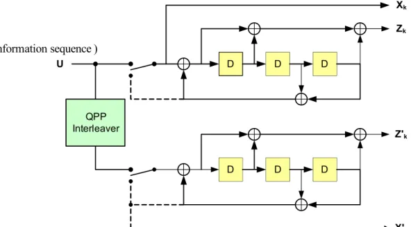
In 3GPP-LTE specification, the scheme of turbo encoder is a Parallel Concatenated Convolutional Code (PCCC) with 8-state constituent encoders and one internal inter-leaver. The coding rate of turbo encoder is 1/3. The structure of turbo encoder is illustrated in Fig. 3.1
D D D U Xk Zk D D D Z'k QPP Interleaver X'k (Information sequence )
Figure 3.1: Turbo encoder for 3GPP-LTE.
The transfer function of the 8-state constituent code for the PCCC is G(D) = · 1, 1 + D + D 3 1 + D2+ D3 ¸ . (3.1)
The bit sequence input for a given code block to channel coding by c0, c1, c2, c3, ...,
cK−1, where K is the number of bits to encode. After encoding, the bits are denoted by
d(i)0 , d(i)1 , d(i)2 , d(i)3 , ..., d(i)D−1, where D is the number of encoded bits per output stream and i indexes the encoder output stream.
The initial value of the shift registers of the 8-state constituent encoders shall be all zeros when starting to encode the input bits. The output from the turbo encoder is d(0)k = xk, d (1) k = zk, d (2) k = z ′
k for k = 0, 1, 2, ..., K − 1. The bits input to the turbo
encoder are denoted by c0, c1, c2, c3, ..., cK−1, and the bits output from the first and
second 8-state constituent encoders are denoted by z0, z1, z2, z3,..., zK−1 and z ′ 0, z ′ 1, z ′ 2, z′ 3, ..., z ′
K−1, respectively. The bits output from the turbo code internal interleaver are
denoted by c′ 0, c ′ 1, c ′ 2, c ′ 3, ..., c ′
K−1, and these bits are to be the input to the second encoder.
Moreover, trellis termination is performed by taking the tail bits from the shift register feedback after all information bits are encoded. Tail bits are padded after the encoding of information bits. The transmitted bits for trellis termination shall be:
d(0)K = xK, d(0)K+1 = zK+1, d(0)K+2 = x ′ K, d (0) K+3 = z ′ K+1 d(1)K = zK, d(1)K+1 = xK+2, d(1)K+2 = z ′ K, d (1) K+3 = x ′ K+2 d(2)K = xK+1, d(2)K+1 = zK+2, d(2)K+2 = x ′ K+1, d (2) K+3 = z ′ K+2
3.2
QPP interleaver
Interleavers for turbo codes have been extensively investigated. In particular, quadratic polynomials were emphasized. The algebraic approach was shown to admit analytical de-sign of an interleaver matched to the constituent codes. The interleaver used in 3GPP-LTE standard is quadratic permutation polynomial (QPP) interleaver [2] [10]. Moreover, the performance using QPP interleaver was shown to be better than S-random interleavers [11] for short-to-medium block lengths. The formula of this interleaver is
π(x) = f1x + f2x2(modN ), (3.2)
where N is the block length and the f1, f2, are the non-negative integers of the QPP
interleaver of different block length. The interleaver parameter f1, f2, will be shown in
detail in Appendix A. Besides, x is the original address and π(x) is the address after interleaving. The algebraic construction can make a contention-free condition.
In recent years, the parallel processing of iterative decoding of turbo codes is of interest for high-speed decoders. Contention-free interleavers have recently been shown to be suitable for parallel decoding of turbo codes. Furthermore, in [12] it was shown that all quadratic permutation polynomials generate maximum contention-free interleavers, i.e., every factor of the interleaver length becomes a possible degree of parallel processing of the decoder. Thus, this class of interleaver is very interesting from an implementation point of view. That is, when multiple MAP decoders try to access multiple memories concurrently, there are no hazards happened.
3.2.1
Contention-free interleaver
To increase throughput, a MAP decoder is parallelized by dividing a size-N trellis into M size-W windows (N=MW) and employing M synchronous MAP-based decoders
with M separate memory banks. Interleavering latency is eliminated by writing the M values generated each clock cycle directly to their interleaved position. However, if the interleaver is not designed well, two or more MAP-based decoders may require access to the same memory bank on a given clock cycle, resulting in a memory contention.
Several interleaving algorithms with contention-free properties [13] have been pub-lished, and the QPP interleaver has the contention-free property. Fig.3.2 shows an exam-ple of memory contention problem in a parallel decoding structure. A codeword sequence is stored in order in four different memory banks. It is obvious that it is a contention-free access at all different timing with pre-permutation order. But it will have the mem-ory contention problem if we apply post-permutations. The post-permutation 1 is a contention-free interleaver design. Because every time we access four symbols, they come from different memory banks. The interleaver design of post-permutation 2 suffers two
access collisions at time T0 and T2. Due to the good property mentioned above, the QPP
interleaver is suitable for parallel decoding of turbo code.
3.2.2
Performance comparison
The design of the interleaver is critical to the performance of the Turbo Code. Inter-leavers can in general be separated into two classes: random interInter-leavers and deterministic interleavers. The basic random interleavers permute the information bits in a pseudoran-dom manner. It was demonstrated in [14] that near Shannon limit performance can be achieved with these interleavers for large frame sizes. The S-random interleaver proposed in [15] is an improvement to the random interleaver. The S-random interleaver is a pseudo-random interleaver with the restriction that any two input positions within distance S cannot be permuted to two output positions within distance S.
QPP interleaver is a class of deterministic interleavers based on a quadratic congruence in (3.2). The interleaver depends on permutation polynomials over the ring of integers modulo N . By carefully selecting the coefficients of the polynomial, we can achieve a performance close to, or in some case, even better than S-random interleavers. The performance result is illustrated in Fig. 3.3.
6 7 4 5 8 9 10 11 12 13 14 15 2 3 0 1 2 3 0 1 6 7 4 5 10 11 8 9 14 15 12 13 6 7 4 13 10 0 9 14 15 12 5 2 3 8 1 11 7 4 13 10 9 14 15 0 5 12 2 3 6 11 8 1 6 7 4 5 10 11 8 9 14 3 1 12 2 0 13 15 8 14 3 1 7 5 12 2 4 9 13 0 6 10 15 11 Pre-Permutation Post-Permutation 1 Post-Permutation 2 Time
Contention
Contention
Contention
Contention----free
free
free
free
Collision
Collision
Collision
Collision
Collision T0 T1 T2 T3Figure 3.2: Example of a contention-free permutation.
3.3
Decoding procedure
According to the iterative decoding algorithm of turbo codes in section 2.2, we realize that the goal of the MAP algorithm is to derive the LLR and extrinsic values. Therefore, for the input signal ut, the LLR can be represented as
L(ˆut) = log
P (ut = +1|r)
P (ut = −1|r)
, (3.3)
where ut is defined as the collection of input symbols (u0,t,u1,t) from time (t − 1) to time
0 0.2 0.4 0.6 0.8 1 1.2 1.4 10−5 10−4 10−3 10−2 10−1
BPSK; AWGN Channel; Iteration=10
Eb/N0 (dB)
BER
Srandom__1024 QPP__1024
Figure 3.3: Performance comparison.
(3.3) will be L(ˆut) = log P (m′,m)∈B+1 t P (St−1 = m ′, S t= m|r) P (m′,m)∈B−1 t P (St−1 = m ′, S t = m|r) = log P (m′,m)∈B+1 t P (St−1 = m ′, S t= m, r) P (m′,m)∈B−1 t P (St−1 = m ′, S t = m, r) = log P (m′,m)∈B+1t αt−1(m ′) · γ t(m′, m) · βt(m) P (m′,m)∈B−1 t αt−1(m ′) · γ t(m′, m) · βt(m) , (3.4)
where B+1t is the set of (m′, m) that indicate the state transitions which are caused by
ut= +1, and B−1t , the set of (m′, m), denoted the state transitions are due to ut= −1.
Applying the Log-MAP algorithm to the (3.4), the LLR can be rewritten to L(ˆut) = log P (m′,m)∈B+1 t e ¯ αt−1(m′)+¯γt(m′,m)+ ¯βt(m) P (m′,m)∈B−1 t e ¯ αt−1(m′)+¯γt(m′,m)+ ¯βt(m) = max (m′,m)∈B+1t ∗{¯α t−1(m′) + ¯γt(m′, m) + ¯βt(m)} − max (m′,m)∈B−1 t ∗{¯α t−1(m′) + ¯γt(m′, m) + ¯βt(m)}, (3.5)
and the Max-Log MAP approximation will become L(ˆut) = max (m′,m)∈B+1 t {¯αt−1(m′) + ¯γt(m′, m) + ¯βt(m)} − max (m′,m)∈B−1 t {¯αt−1(m′) + ¯γt(m′, m) + ¯βt(m)}. (3.6)
Furthermore, the initial condition of branch metrics become ¯
α0(0) = 0, α¯0(m) = −∞ for m 6= 0
¯
βN(0) = 0, β¯N(m) = −∞ for m 6= 0
(3.7)
For a rate 1/n RSC encoder, each codeword frame consists of one systematic bit and (n − 1) parity bits. In the receiver, the received codeword has the systematic symbol r(0)t abd parity symbols r
(1)
t ∼ r
(n−1)
t . Moreover, in order to reduce the computational
complexity, we could further simplify the path metrics into
¯ γt(m′, m) = 1 2(utLa(ut) + Lcutr (0) t + n−1 X i=1 Lcr(i)t vt(i)), (3.8)
where the value of vt(i) ∈ {+1, −1} depends on the encoding generator matrix after
BPSK mapping. Lc is the channel reliability value for the AWGN channel. The a priori
information in (3.8) is represented by La(ut) ∆ = logP (ut= +1) P (ut= −1) . (3.9)
From the decoding flow shown in Fig. 2.4, the extrinsic information corresponding to the information bit ut for the next stage can be calculated as
Le(ut) = L(ut) − Lcr0,t− La(ut). (3.10)
Computer symbol probabilities for the next decoder from previous decoder as La(ut) = Le(˜ut) = log
P (ut = +1)
P (ut = −1)
. (3.11)
Assume the information symbols are equal probability, so the a priori information can be initialized for the first iteration:
log P (ut= +1) = 0 log P (ut= −1) = 0 (3.12)
The turbo decoding proceeds iteratively with the extrinsic information passing between the two SISO decoders. When the stopping criteria is reached, which may be the maximum iteration number or a correctly decoded codeword, the final decisions after de-BPSK are
ut= 0, if L(ut) ≥ 0 1, otherwise (3.13)
3.4
Design parameter analysis
In this section, we will present the simulation results and some parameters setting for implementation. All the simulation results are signal-to-noise (SNR) versus BER under BPSK modulation and AWGN channel.
In order to determine appropriate design parameters such as the bit widths of the input symbol, the branch metric, and the path metric, the performance evaluation through simulations are necessary. The iteration number and the sliding window size will directly influence not only the performance of turbo coding but also the hardware cost of the design. The BER curves of the floating point decoders under BPSK modulation and AWGN channel with block length of 2048 are presented in Fig. 3.4. In Fig. 3.4, there is
a 0.05dB loss between the sliding window size of 16 and 32 at the BER=10−5 under the
fixed 8 iterations. Therefore, we choose the window size 16 in our design.
However, the Max-Log MAP decoding algorithm can reduce the decoding complexity, it causes the performance loss due to the approximation of max function. The scaling factor approach [16] is applied as compensation for the performance loss due to the Max-Log-MAP algorithm. That is, a scaling factor to scale down the extrinsic information is introduced. Therefore, the intrinsic information La(ut) can be formulated as :
La(ut) = β × Le(˜ut), (3.14)
where β is the scaling factor. We choose the scaling factor β=0.75 in our design for performance compensation. This approach not only improves the performance but also cost a little gate counts.
The fixed point representation of the internal variable in the SISO decoder is deter-mined from the received symbol quantization. Fig. 3.5 shows the simulation result with different input symbol quantization under BPSK modulation and AWGN channel, and we
0 0.2 0.4 0.6 0.8 1 1.2 1.4 10−6 10−5 10−4 10−3 10−2 10−1 100
BPSK; AWGN Channel; Block length 2048; Iteration 8
Eb/N0 (dB)
BER
Window size 8 Window size 16 Window size 32
Figure 3.4: Comparison of window size.
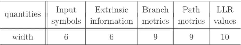
choose block length 2048, window size 16, and iteration number 8. Note that a.b in the figure denotes the quantization scheme where a is the integer part, and b is the fractional part. Furthermore, the primary specifications of MAP decoder are given in Table 3.1, where the code polynomial is follow 3GPP-LTE system.
Table 3.1: MAP Decoder Specification generator matrix [ 1 1+D1+D+D2+D33 ]
code rate 1/3
sliding window size 16
We can observe that the quantized format 6 bits (3.3) is suitable scheme for our design. In addition, the width of extrinsic information, branch metric, and path metric can be derived and we summarize the fixed representations in Table 3.2.
In 3GPP-LTE specification, there are 188 different block lengths based on particular QPP parameters. The shortest size and the longest one are 40 and 6144, respectively. The
0 0.2 0.4 0.6 0.8 1 1.2 1.4 10−6 10−5 10−4 10−3 10−2 10−1 100
BPSK; AWGN Channel; Block length 2048; Iteration 8
Eb/N0 (dB)
BER
fixed−3.2 fixed−3.3 floating
Figure 3.5: Fixed point comparison.
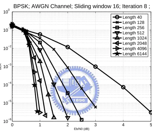
performance of different size is apparently distinct during simulation and is illustrated in Fig. 3.6. The parameters of simulation is under 8 iterations and sliding window size 16.
In Fig. 3.6, we can see that the worst case (N=40) can achieve BER=10−5 at SNR about
4.5 ∼ 5.0 dB and the best one (N=6144) can reach the same BER under 1.0 dB. Table 3.2: Summary of fixed representation in MAP decoder
quantities Input Extrinsic Branch Path LLR
symbols information metrics metrics values
0 1 2 3 4 5 10−6 10−5 10−4 10−3 10−2 10−1 100
BPSK; AWGN Channel; Sliding window 16; Iteration 8 ;
Eb/N0 (dB) BER Length 40 Length 128 Length 256 Length 512 Length 1024 Length 2048 Length 4096 Length 6144
Chapter 4
Reconfigurable 3GPP-LTE Turbo
Decoder
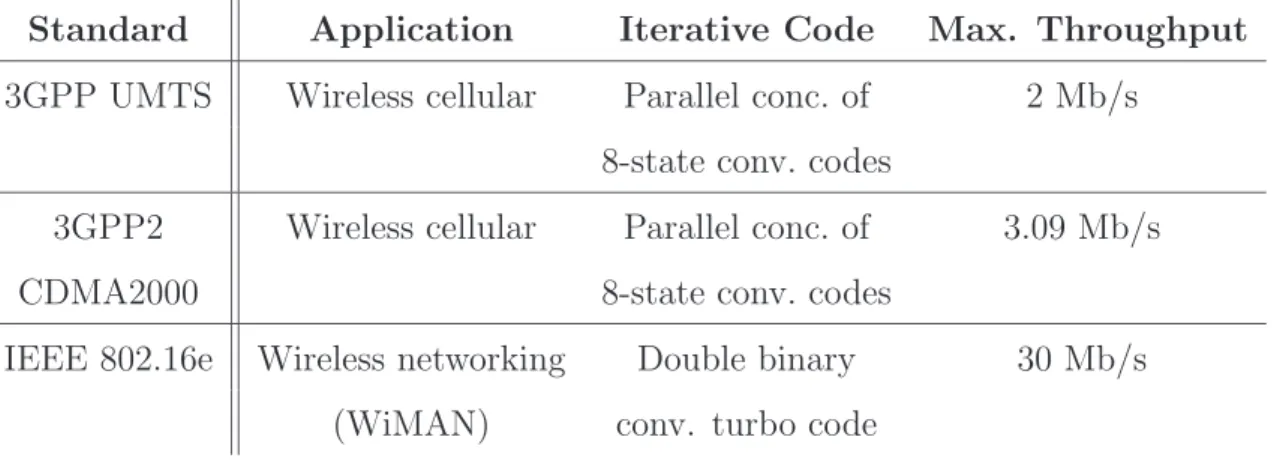
The turbo codes have found applications in several standards listed in Table 4.1 due to its outstanding error correction ability. However, several communication application in the future may demand for a higher speed channel coding scheme. It may become a obstacle for turbo codes in hardware implementations.
To meet the future applications, we proposed a parallel architecture of turbo decoder for improving the throughput. In this chapter, not only the proposed turbo decoder but also the MAP decoder utilized in our architecture will be described in detail. Moreover, since the block length ranges from 40 to 6144, the memory requirement is also a great issue. A residue-only interleaver is adopted to reduce storage memory. Furthermore, reconfigurable property of our decoder designed for applying in various situation will also
Table 4.1: Standard specifications for turbo coding
Standard Application Iterative Code Max. Throughput
3GPP UMTS Wireless cellular Parallel conc. of 2 Mb/s
8-state conv. codes
3GPP2 Wireless cellular Parallel conc. of 3.09 Mb/s
CDMA2000 8-state conv. codes
IEEE 802.16e Wireless networking Double binary 30 Mb/s
be introduced later. Finally, how to compute the throughput in our parallel architecture will be interpreted clearly.
4.1
Architecture overview
According to the turbo decoding flow shown in Fig. 4.1, each iteration computes the extrinsic information which is an a priori value estimation for the next iteration. The next iteration remains idle until the interleaving step reorders all decoding results. The latency and the performance are determined by the iteration number and the block size. In the conventional turbo decoder, lower error rate can be achieved with large block size, but it also requires more decoding time. Hence, the application of turbo code provides a trade-off between performance and speed.
YES Output Decision Bits NO Iterative Decoding LLR & Extrinsic Information Calculation Stopping Criterion Interleaving / Deinterleaving A Priori Probability Estimation Initialization Decoder
Figure 4.1: Iterative decoding flow of turbo decoder.
Fig. 4.2 shows the simple block diagram of proposed parallel decoder. There are 8 radix-2 MAP decoders and 8 memory banks connected with QPP network and parallel network [17]. Each memory stores the required data for decoding, including the received LLR values from channel and the extrinsic informations from MAP decoder. Each MAP decoder computes the a priori probability which is used in the next decoding round and makes decision for received symbols. The interleaver is implemented with the address generators inside each memory and the global network controller, then the pseudo random data will be fed into the MAP decoders. In addition, the decoder supports 188 kinds of
block length, 40 ∼ 6144, and all the QPP interleaver parameters f1 and f2. Iteration
numbers in this design also can be worked from 1 ∼ 8. The detail process and architecture is explained in the following subsection.
Memories*8
Decoders*8
QPP Network
Output Buffer Input Buffer
Figure 4.2: Block diagram of proposed turbo decoder.
4.2
MAP decoder
4.2.1
Decoding schedule
Fig. 4.3 presents the radix-2 MAP decoder, which consists of branch metric unit(BMU), add-compare-select (ACS) unit, log-likelihood-ratio (LLR) unit and input buffers (IBUF). The input buffers are used to store the input symbols. The BMUs calculate the branch
metrics for α-ACS, β-ACS, and βd-ACS units and each ACS unit according to the trellis
structure performs addition, comparison, and selection. The α-ACS unit carries out the forward recursion and saves the result in the α-buffer. β-ACS unit begins the backward
recursion from the initial conditions determined by the βd-ACS unit calculation.
More-over, the α-buffer performs the Last-In/First-Out (LIFO) in order to reorder the α value
for LLR calculation. The LLR unit determines the LLR values L(ut) used to make
deci-sion and the extrinsic informations Le(ut) that store in the memory for the next decoding
IBUF_1 -BMU -BMU -ACS -ACS LLR
β
β
α
IBUF_2 -BMU -ACSα
α
β
d dβ
-bufferFigure 4.3: Block diagram of MAP decoder.
To consider the sliding window approach shown in Fig. 2.7, the backward metric β evaluation can be started until the required window of data have been stored. However,
if we reverse the order of input sequence within a sub-block, the input buffer of the βd
computation can be saved [19]. Fig. 4.4 is the decoding schedule of the MAP decoder. In
order to reduce the IBUF for βd-ACS, the input sequence order of decoding is from the
end of the sliding window to the beginning of the window. That is, the input sequences
are written into the input buffer in the reversed order. In Fig. 4.4, the βd computation
can be executed immediately at the first time interval since the reversed sequence. Then the α recursion is performed on the previous stored data at the next time interval and the second window data will be written into the other input buffer. Finally, the first window data will be read at the third time interval for backward β calculation at the same and
the third window data will be written into the input buffer simultaneously. When the first window β starts to calculate, the LLR computation also calculates in a neglected latency. As a result, the latency of MAP decoder is about two sliding window size.
β
α
α
α
α
W0 W1 W3 W2 T0 T1 T2 ... Time interval T3 BMU -ACS -ACS -ACS LLR d βα
β dβ
dβ
dβ
dβ
β
β
β
Figure 4.4: Decoding schedule of MAP decoder.
4.2.2
The circuit for LLR calculation
Our design adopts the modulo normalization to avoid overflow of path metric [20]. This methods requires only one more bit in the ACS unit and a simple modification inside the LLR unit. Only the differences between both forward path metric and backward path metric are significant in modulo normalization, so the LLR unit has to use these differences to calculate the log-likelihood value. We rearrange the computation order of log-likelihood value from circuit in Fig. 4.5(a) to Fig. 4.5(b). Although the two circuits have the same function, the original circuit may result in overflow due to the limited data width. The modified circuit could guarantee the correctness and cause no extra path delay.
4.3
Proposed Turbo decoder design
Fig. 4.6. shows the block diagram of proposed decoder, which consists of 8 parallel decoders and 8 memory sets. For an example of block length 1024, we separate a code-word into 8 sub-blocks with length 128. Each sub-block is assigned to one decoder and
1 0 1 0
(
α α
−
) (
+
β β
−
)
1α
0α
β
0β
1 (b) Modified 1α
0α
β
0β
1 (a) Original 1 1 0 0(
α β
+
) (
−
α β
+
)
Figure 4.5: The circuit for LLR unit.
decoded separately. These sub-blocks are connected by a well-designed QPP interleaver. This method avoids the forward and backward recursion problem while using parallel architecture. The decoding process is described as follows: each memory will collect a 128-bits sub-block from input buffer until the whole 1024-bits codeword is received. The memory stores the received symbols and extrinsic information, and the 8 memories will deliver the required data to the 8 MAP decoders through QPP network. The interleaver is implemented with the address generators in each memory and the network controller. The MAP decoders perform the primary decoding procedures, and each one decodes the sub-blocks. After the required iterations, our design will output the decisions of current block and start to decode next block.
As described in the previous section, the quadratic permutation polynomial interleaver interchanges the information between each blocks to improve performance. In addition, the quadratic permutation polynomials generate the contention-free interleavers. There-fore, we can access the required data from different memory banks without memory con-tention and decoding several blocks in parallel to reduce the large decoding latency. Each MAP decoder is based on the Max-Log-MAP algorithm and adopted the radix-2 ACS structure. The memory blocks are used for data storage, which store the input informa-tion and extrinsic values generated by the MAP decoder. Note that the number of MAP decoders and memory banks are the same, which is because that each decoder can access data from memory in a one-to-one mapping condition at the same time. Eventually, the
network is a permutation control unit which controls the interchange of both the input symbols and extrinsic informations. In the following subsection, we will also introduce the characteristic of our design and the throughput calculation in detail.
Q u a d ra tic P e rm u ta ti o n P e rm u ta tio n N e tw o rk In p u t B u ffe r MAP_00 MAP_01 MAP_06 MAP_07
…………
…………
MEM_00 MEM_01 MEM_06 MEM_07…………
…………
Control O u tp u t B u ffe rFigure 4.6: Proposed turbo decoder architecture.
4.3.1
Residue-only interleaver
From the QPP interleaver formula, f (x) = f1x + f2x2(modN ), the algebraic
construc-tion makes a contenconstruc-tion-free condiconstruc-tion. A mathematical descripconstruc-tion of contenconstruc-tion-free condition is now given. The exchange and processing of a sequence of N = M W symbols between sub-blocks of the iterative decoder can be parallelized by M processors working on window sizes of length W in each sub-block provided that the following condition holds for the interleaver f (x), 0 ≤ x ≤ N :
where 0 ≤ j < W , 0 ≤ t < v < N/W , and π(·) is f (·). First, it verifies the equation (4.1) for f (x). Let Qt= ¹ f (j + tW ) W º ,Qv = ¹ f (j + vW ) W º , (4.2) then f (j + tW ) = QtW + [f (j + tW )(modW )] f (j + vW ) = QvW + [f (j + vW )(modW )] . (4.3)
It must show that Qt 6= Qv for t − v 6= 0(modM ) and any 0 ≤ j < W . Assume
Qt= Qv, then
Qt− Qv =
f (j + tW ) − [f (j + tW )(modW )] − f (j + vW ) − [f (j + vW )(modW )]
W = 0.
(4.4) Using the simple proposition below:
P roposition: Let M be an integer. Support that M |N and that x ≡ y (mod N ). Then x ≡ y (mod M ).
Observing that
f (j + tW ) ≡ f1j + f2j2(modW ), f (j + vW ) ≡ f1j + f2j2(modW ). (4.5)
It can conclude that
[f (j + tW )(modW )] = [f (j + vW )(modW )] . (4.6)
Therefore, the absolute value of equation (4.4) can be simplified as |Qt− Qv| =
[f (j + tW )] − [f (j + vW )]
W = 0. (4.7)
By noting that (j + tW ) 6= (j + vW ) and that f (x) is a permutation polynomial, concluding f (j + tW ) 6= f (j + vW ) and having a contradiction in (4.7).
From the equation (4.5) and (4.6), we know that the residue part of the address calcu-lation will be the same. That is, when using QPP interleaver in the parallel construction, the residue address of each memory bank is the same. It will be very helpful to our design. Because the longest block length is 6144 and multiple memory banks, the memory costs are too much. For this reason, we use the residue-only interleaver in our design, and the residue address can be repeatedly used in different memory banks. Only the residue ad-dress has to be saved instead of total adad-dress, leading to reduce the memory costs largely.
Fig. 4.7 shows a 4 MAP decoders and 4 memory banks example, we can see that each MAP decoder access data from the same address of each memory but different memory bank. The residue address will be the same after calculation in the right of Fig.4.7.
x ) (x π MAP decoder Memory bank 3 1 2 0 3 1 2 0 6 7 5 4 6 7 5 4 8 9 10 11 8 9 10 11 12 13 14 15 12 13 14 15 0 7 10 1 4 11 14 5 8 15 2 9 12 3 6 13 7÷4=1⋯3 2 2 4 10÷ = ⋯ 0 0 4 0÷ = ⋯ 1 0 4 1÷ = ⋯ 0 1 4 4÷ = ⋯ 1 1 4 5÷ = ⋯ 3 2 4 11÷ = ⋯ 2 3 4 14÷ = ⋯ 0 2 4 8÷ = ⋯ 1 2 4 9÷ = ⋯ 3 3 4 15÷ = ⋯ 2 0 4 2÷ = ⋯ 2 1 4 6÷ = ⋯ 0 3 4 12÷ = ⋯ 1 3 4 13÷ = ⋯ 3 0 4 3÷ = ⋯
Figure 4.7: Example of residue-only interleaver.
4.3.2
Reconfigurable 1/2/4/8-MAP decoders
From the observation of the QPP parameter in Appendix A, the block length can be classified as following: N = 40 + 8a, 0 ≤ a ≤ 59 512 + 16b, 0 < b ≤ 32 1024 + 32c,0 < c ≤ 32 2048 + 64d,0 < d ≤ 64 (4.8)
There are all 188 modes, and each block size can be divided by 1, 2, 4, and 8 at most. In this opinion, we design a reconfigurable MAP decoder numbers in our architecture. Because of parallel decoding, a received codeword is partitioned into 8 memory banks. Therefore, we can decode the received codeword by utilizing 1-SISO, 2-SISO, 4-SISO or 8-SISO respectively, based on the block length, performance or throughput expected. It can be illustrated in Fig. 4.8.
In order to satisfy the 3GPP-LTE block length requirement, there are some compro-mises between performance and area cost for all block size. Fig. 4.9 shows the perfor-mance of the shortest size 40 with different MAP decoders. In Fig. 4.9, we can see that the performance curve of using 8-SISO decoders even 4-SISO or 2-SISO is worse than using 1-SISO. First, we would like to figure out how the performance degrades and then
Memories Decoders QPP Network Output Buffer Input Buffer 8-SISO Memories Decoders QPP Network Output Buffer Input Buffer 4-SISO Memories Decoders QPP Network Output Buffer Input Buffer 2-SISO Memories Decoders QPP Network Output Buffer Input Buffer 1-SISO
Figure 4.8: Decoding codeword with various processing elements.
we can find some approaches to improve it. The degradation of performance may be formed by two factor: the first one is that the small section size cause the shorter trellis structure. Therefore, the calculation of path metric α or β will be unreliable to make the final decision. The second is the boundary initial value. In general, we often set the initial value of each state to be zero in every boundary. Nevertheless, the performance loss can not be obviously found on decoding long block size with multiple SISO decoders. Because there are fewer such problems mentioned above for long block length.
The warm-up free method [21] is applied to improve performance degradation in our design. In this method, a warm-up free parallel architecture is proposed by using the α path metrics that were calculated in the previous iteration of the adjacent sub-block to initialize the path metrics for each sub-block in the next iteration. That is, the α path metrics of the last information bit in sub-block i were stored for initialization of the forward path metrics of the sub-block (i + 1) in the next iteration. In the first iteration, the initial values of α path metrics needed in the next iteration are not available, thus the initial values will be set to zero.
After adoption of this method, the forward path metrics become more reliable. There-fore, the performance can be improve with multiple SISO decoders for short block length. Fig. 4.10 shows the final performance of our design of size 40. Comparing with Fig. 4.9, the performance of using multiple SISO decoders is near the performance of utilizing 1-SISO. Moreover, the performance of decoding long block size with different SISO decoder
0 1 2 3 4 5 6 10−6 10−5 10−4 10−3 10−2 10−1 100
BPSK; AWGN Channel; Turbo Codes ;
Eb/N0 (dB) BER BL40__8−SISO BL40__4−SISO BL40__2−SISO BL40__1−SISO
Figure 4.9: Short block length 40 of 1/2/4/8-SISO decoders without warm-up free method.
is almost close. It can be shown in Fig. 4.11 with a long size 6144.
In the following, we will also show some simulation results for the iteration consider-ation. Because we depend on two reasons: the first one is that the all block lengths are
from 40 to 6144, and the needed iterations may be different at BER=10−5 under AWGN
channel. The second is about throughput computation. Fewer iteration numbers we use, the higher throughput we achieve. For the iterative decoding process, increasing the iter-ation numbers may cause the performance curve to converge eventually and the required iterations can be obtained. The performance of different lengths and iterations are illus-trated in Fig. 4.12 and 4.13. In Fig. 4.12 and 4.13, we can figure out that the shorter lengths need fewer iterations to converge, but the longer ones require more. Finally, we can derive the summary in Table 4.2.
Therefore, the numbers of iteration are so flexible for all block length in our design. That is to say, our turbo decoder can support the iteration numbers from 1 ∼ 8.
0 1 2 3 4 5 6 10−6 10−5 10−4 10−3 10−2 10−1 100
BPSK; AWGN Channel;Block length 40;Iteration 8
Eb/N0 (dB) BER 8−SISO decoders 4−SISO decoders 2−SISO decoders 1−SISO decoder
Figure 4.10: Performance comparison of size 40 of 1/2/4/8 decoders with warm-up free method.
4.3.3
Throughput consideration
In this section, we will introduce how to computer the throughput. There are some critical factors affecting the result. The throughput is defined as decoding how many bits per second. In the parallel architecture, the function can be translated in equation (4.9). Each factor will interpret as following: f is the operating frequency, which means the inverse of the critical path of our design. Moreover, the critical path in general resides in the ACS unit. For trellis-based 3GPP-LTE decoder, each state receives two branch metrics and also sends two messages to other states. As a result, radix-2 ACS unit is
Table 4.2: Needed iterations of different size
Block length Needed iteration
40-512 3 or 4
512-2048 5 or 6
0 0.2 0.4 0.6 0.8 1 10−6 10−5 10−4 10−3 10−2 10−1 100
BPSK; AWGN Channel;Block length 6144 ;Iteration 8
Eb/N0 (dB) BER 8−SISO decoders 4−SISO decoders 2−SISO decoders 1−SISO decoder
Figure 4.11: Performance comparison of size 6144 of 1/2/4/8 decoders with warm-up free method.
required to decode the trellis structure. In order to diminish the critical path ,only radix-2 structure is considered in our design. It also means that the decoder can decode one bit each time. That is, the Radixf actor in equation (4.9) is 1. P arallel is the number of decoders which are used to decode. As we know, the more decoders, the higher throughput can be derived. But the cost may be increased oppositely. The maximum decoders in our architecture are 8. The significant factor effecting the throughput is the ef f iciency of each MAP decoder. From the decoding schedule in Fig. 4.4, we realize that there are about three sliding window size latency in each decoding round. The decoder actually starts to decode in the third time interval. Thus the efficiency is formed in equation (4.10). Decoding with 1-SISO, 2-SISO, 4-SISO, and 8-SISO , the efficiency of each SISO decoder may be different. The efficiency in all case is shown in Table 5.1. The final factor is the number of iterations. Based on MAP decoding algorithm, the decoding process through pre-decoding round and post-decoding round is called one iteration. That is why the denominator of equation (4.9) are two times of iterations. Based on all factors mentioned
0 1 2 3 4 5 10−6 10−5 10−4 10−3 10−2 10−1 100
BPSK; AWGN Channel; Different Iteration
Eb/N0 (dB) BER 40__ite=2 40__ite=4 40__ite=6 40__ite=8 0 0.5 1 1.5 2 10−6 10−5 10−4 10−3 10−2 10−1 100
BPSK; AWGN Channel; Different Iteration
Eb/N0 (dB) BER 512__ite=2 512__ite=4 512__ite=6 512__ite=8
Figure 4.12: Performance of size 40 and 512 under various iterations.
0 0.2 0.4 0.6 0.8 1 1.2 1.4 10−6 10−5 10−4 10−3 10−2 10−1 100
BPSK; AWGN Channel; Different Iteration
Eb/N0 (dB) BER 2048__ite=2 2048__ite=4 2048__ite=6 2048__ite=8 2048__ite=10 0 0.2 0.4 0.6 0.8 1 10−6 10−5 10−4 10−3 10−2 10−1 100
BPSK; AWGN Channel; Different Iteration
Eb/N0 (dB) BER 6144__ite=2 6144__ite=4 6144__ite=6 6144__ite=8 6144__ite=10
Figure 4.13: Performance of size 2048 and 6144 under various iterations.
above, the throughput can be evaluated eventually. The throughput of our design will show in the next chapter in Table 5.2.
T hroughput(bits/s) = N eeded cyclesBlock Length × clock rate
= Block Length
decoding round# × decoding round#cycle × time cycle
= f ×
Block Length cycle per decoding round
decoding round#
= f ×
Radix f actor×P arallel×real decoding cycle cycle per decoding round
decoding round#
= f × Radix f actor × P arallel × ef f iciency
• f : Operation f requency
• Radix factor : Radix structure of ACS unit • Parallel : P arallel decoder numbers
• efficiency : decoding ef f iciency of each M AP decoder • iteration : number of iterations
ef f iciency = real decoding cycle
Chapter 5
Implementation Results
5.1
Chip characteristic
As described in section 4.3.3, the efficiency of each SISO decoder with 1/2/4/8-decoders is different. It can be calculated from equation (4.10). Table 5.1 shows the efficiency results in all case. In Table 5.1, we know that when block length becomes longer, the efficiency also becomes larger. Moreover, the efficiency of decoding the long block size with 1-SISO and 8-SISO decoders becomes close.
Based on the MAP efficiency results, we can use equation (4.9) to compute the through-put. In our design, the operation frequency can reach 277MHz. The needed iteration num-bers can estimate from the performance simulation. Therefore, the throughput summary is shown in Table 5.2.
Based on the architectures described in chapter 4, we proposed a reconfigurable turbo Table 5.1: Efficiency of each SISO decoder with 1/2/4/8-decoders
1/2/4/8-SISO decoders
Block length each decoder each decoder each decoder each decoder
of 1-SISO of 2-SISO of 4-SISO of 8-SISO
40 0.465 0.303 0.227 0.172
512 0.917 0.847 0.735 0.581
2048 0.978 0.957 0.917 0.847