An application of non-normal process capability indices

AN APPLICATION OF NON-NORMAL PROCESS

CAPABILITY INDICES

k. s. chen and w. l. pearn*

Department of Industrial Engineering & Management, National Chin-Yi Institute of Technology, Taichung, Taiwan ROC

Department of Industrial Engineering & Management, National Chiao Tung University, Hsinchu, Taiwan 30050 ROC

SUMMARY

Numerous process capability indices, including Cp, Cpk, Cpm, and Cpmk, have been proposed to provide measures of process potential and performance. In this paper, we consider some generalizations of these four basic indices to cover non-normal distributions. The proposed generalizations are compared with the four basic indices. The results show that the proposed generalizations are more accurate than those basic indices and other generalizations in measuring process capability. We also consider an estimation method based on sample percentiles to calculate the proposed generalizations, and give an example to illustrate how we apply the proposed generalizations to actual data collected from the factory.  1997 John Wiley & Sons, Ltd.

key words: process capability index; process mean; process standard deviation; percentile

1. INTRODUCTION butions. In this paper, we consider some generaliza-tions of those basic indices to cover non-normal Process capability indices (PCIs) have been widely

distributions. Comparisons on accuracy of the capa-used in the manufacturing industry, to provide a

bility measurement between the basic indices and numerical measure on whether a process is capable

the proposed generalizations are provided. of producing items meeting the quality requirement

preset in the factory. Numerous capability indices

have been proposed to measure process potential _{2. THE INDICES C}

p(u,v)

and performance. Examples include the two most

commonly used indices, Cp and Cpk discussed in Va

¨

nnman9 _{constructed a superstructure for the four}

Kane1_{, and the two more-advanced indices C}

pm and basic indices, Cp, Cpk, Cpm, and Cpmk. The

super-Cpmk developed by Chan et al.2 and Pearn et al.3 structure has been referred to as Cp(u,v), which can

There are many other indices but they can be viewed be defined as the following: as modifications of the above four basic indices (see

Boyles4

, Pearn and Chen5

and Zwick6 ). Cp(u,v)= d−uum−mu 3

Î

s2_{+ v(}m−_T)2 , (1)

Discussions and analysis of these indices on point estimation and construction of confidence intervals have been the focus of many statistician and quality researchers including Kane,1 _{Chan et al.,}2 _{Chou et}

where m is the process mean, s is the process

al.,7 _{Pearn et al.,}3 _{Kotz et al,}8_Va¨_nnman,9 _{Pearn and}

standard deviation, d= (USL−LSL)/2 is half of the

Chen,10_{and many others. Most of the investigations,}

length of the specification interval, m=

however, depend heavily on the assumption of nor- (USL+LSL)/2 is the mid-point between the upper mal variability. If the underlying distributions are and the lower specification limits, T is the target non-normal, then the capability calculations are value, and u, v$ 0. It is easy to verify that highly unreliable since the conventional estimator S2

Cp(0,0) = Cp, Cp(1,0) = Cpk, Cp(0,1) = Cpm, and

of s2 _{is sensitive to departures from normality, and}

Cp(1,1) = Cpmk which have been defined explicitly

estimators of those indices are calculated using S2

as: (see Chang et al.,11 _Gunter,12 _{and Somerville and}

Montgomery13

). Therefore, those basic indices are

Cp=

USL−LSL

6s ,

inappropriate for processes with non-normal

distri-*Correspondence to: W.L. Pearn, National Chiao Tung University, _C

pk=min

H

USL−m

3s ,

m−LSL

3s

J

, 1001 Ta Haueh Road, Hsin Chu, Taiwan 30050, ROC

CCC 0748–8017/97/060355–06 $17.50 Received 12 August 1996

ation s by (F99.865−F0.135)/6 in the definition of

Cpm=

USL−LSL

6

Î

s2_{+ (}m−_T)2

, _{the basic indices C}

p(u,v). The idea behind such

replacements is to mimic the property of the normal distribution for which the tail probability outside the

Cpmk=min

H

USL−m

3

Î

s2_{+ (}m−_T)2

, m−LSL 3

Î

s2 _{+ (}m−_T)2

J

. _{63s limits from m is 0.27%, thus assuring that if} the calculated value of CNp(u,v)=1 (assuming the

process is well-centred, or on-target) the probability The index Cp only considers the process varia- that process is outside the specification interval

bility s thus provides no sensitivity on process (LSL, USL) will be negligibly small. It should be departure at all. The index Cpk takes the process noted that the median M is a more robust measure

mean into consideration but it can fail to distinguish of central tendency than the mean m, particularly, between on-target processes from off-target pro- for skewed distributions with long-tails.

cesses (Pearn et al.3_{). The index C}

pm takes the By setting (u,v) = (0,0), (0,1), (1,0), and (1,1),

proximity of process mean from the target value we obtain the following generalizations of the four into account, and is more sensitive to process depar- basic indices for non-normal distributions, which we ture than Cp and Cpk. The index Cpmk adds an refer to as CNp, CNpk, CNpm, and CNpmk:

addition term (m−T)2 _{in the definition, as a penalty}

to the process quality due to the departure of process

CNp=

USL−LSL F99.865−F0.135

, mean from the target value. This additional penalty

ensures that Cpmkwill be more sensitive to departure

than Cpkand Cpm, and therefore is able to distinguish

better between off-target and on-target processes. CNpk=min

5

USL−M

F

F99.865−F0.135 2

G

, M−LSL

F

F99.865−F0.135 2

G

6

, Clearly without the term (m-T)2 _{in the denominator,}

the index Cpmkbecomes Cpk. The ranking of the four

basic indices, in terms of sensitivity to departure of

CNpm= USL−LSL 6

!

F

F99.865−F0.135 6

G

2 + (M−T)2 , process mean from the target value, from the most

sensitive one up to the least sensitive are (1) Cpmk,

(2) Cpm, (3) Cpk, and (4) Cp.

Estimators of the indices Cp(u,v) may be obtained

by replacing m by the sample mean X=(Sn i=1Xi)/n,

and s2

by the sample variance S2 =

(n−1)−1Sn

i=1(Xi−X)

2 _{in definition (1). For normal}

CNpmk=min

5

USL−M 3

!

F99.865−F0.135 6

G

2 + (M−T)2 , distributions, those estimators based on X and S2_,

are quite stable and reliable. But, for non-normal distributions, those estimates become highly unstable since the distribution of the sample variance, S2_{, is}

sensitive to departures from normality, and esti-mators of those indices are calculated using S2_{, as}

pointed out by Chan et al.11 _Gunter,12 _{and Somer-} M−LSL

3

!

F

F99.865−F0.135

6

G

2

+ (M−T)2

6

. ville and Montgomery13 _{demonstrated the strong}

impact this has on the sampling distribution of Cpk.

The ranking of the four generalized indices (when 3. THE GENERALIZATIONS CNp(u,v) _{applied to non-normal distributions) in terms of}

sensitivity to departure of process median from the To accommodate cases where the underlying

distri-target value, from the most sensitive one up to the butions may not be normal, we consider the

follow-least sensitive turns out to be the same. They are ing generalizations of Cp(u,v), which we refer to as

(1) CNpmk, (2) CNpm, (3) CNpk, and (4) CNp. In the

CNp(u,v). The generalizations CNp(u,v) can be

special case where the underlying distribution is defined as (in superstructure form):

normal, then M=m, and F99.865−F0.135=6s. Clearly,

the generalizations CNp(u,v) reduce to the basic

indi-CNp(u,v)= d−uuM−mu 3

!

F

F99.865−F0.135 6

G

2 + v(M−T)2

, (2) ces Cp(u,v), and so CNp = Cp, CNpk = Cpk, CNpm =

Cpm, and CNpmk = Cpmk.

Recently, Zwick,6

and Schneider et al.14

con-sidered two generalizations of Cp and Cpk, which

are similar to CNp, and CNpkbut with process mean

where F_a is the ath percentile, M is the median of

the distribution, m = (USL+LSL)/2 is the mid-point m rather than process median M in the definitions. Extending their definitions to include the other two between the upper and the lower specification limits,

and u, v$ 0. Thus, in developing the generalizations basic indices, Cpmand Cpmk, a superstructure can be

constructed in the following, which we refer to we have replaced the process mean, m, by the

Figure 1. Distributions of processes A, B, and C

Table I. Characteristics of processes A, B, and C _{percentage comparisons, 61% versus 39%, displayed}

in Figure 1 will be replaced by 62% versus 38%.

Process m M s x2

0.135 s299.865 _{Table III is a comparison between the proposed}

generalizations CNp(u,v) and other generalizations

A 10.00 9.37 2.45 7.03 22.63

CNp9(u,v) on the three processes depicted in Figure 1.

B 17.80 17.70 2.45 14.83 30.43

The index values CNp9(u,v) given to processes A and

C 25.60 24.97 2.45 22.63 38.23

C are the same (1.00, 0.00, 0.32, 0.00) for both A

and C), which inconsistently measure process capa-bility in this case.

CNp9 (u,v)= d−uum−mu 3

!

F

F99.865−F0.135 6

G

2 + v(m−T)2 . (3) 5. CALCULATIONS OF CNp(u,v)

Pearn and Chen5 _{proposed an estimator for}

calculat-ing the indices Cp(u,v) assuming the underlying

distributions are Pearsonian types. The estimators

4. COMPARISONS

essentially apply Clements’ method15 _{by replacing}

To compare the proposed generalizations CNp(u,v)

the 6s interval length by Up−Lp, which can be

with Cp(u,v), we consider an example of three

pro-calculated based on available sample data collected cesses A, B, and C depicted in Figure 1. All three

from a stable process utilizing estimates of the mean, processes are distributed as x2 _{with three degrees}

standard deviation, skewness and kurtosis. Under of freedom (a skewed distribution). The

character-the assumption that character-these four parameters determine istics are summarized in Table I (sA = sB = sC = _{the type of the Pearson distribution curve, the F}

a (6)1/2_{). Process B is on-target (}m

B=T), but pro- _{percentiles of the Pearson curves as a function of}

cesses A and C are severely off-target (mA = LSL _{skewness and kurtosis can be calculated utilizing}

and mC = USL). _{the tables provided by Gruska et al.}16 _Those

esti-Table II is a comparison between Cp(u,v) and _{mators can be written as (see Pearn and Chen}5_):

CNp(u,v) on the three processes A, B, and C depicted

in Figure 1. The Cp, Cpk, Cpmand Cpmk values given

to processes A and C are the same. Both processes C˜Np(u,v)=

d−uuMˆ−mu 3

!

F

Up−Lp 6

G

2 + v(Mˆ−T)2 , (4)

are severely off-target. But, the proportion of non-conforming is 61% for process A, which is signifi-cantly greater than that for process C (which is

39%). Obviously, the basic indices Cp(u,v) inconsist- where Up estimates the 99.865 percentile F99.865, Lp

estimates the 0.135 percentile F0.135, and M

ˆ

estimates ently measure process capabilities of processes A

and C in this case. On the other hand, the proposed the median M. To obtain the values of Up, Lp, and

Mˆ tables from Gruska et al.16 _{along with some}

generalizations CNp(u,v) clearly differentiate

pro-cesses A and C by giving smaller values to A and interpolation calculations are required.

Based on sample percentiles, Chang and Lu17

larger values to C (excluding CNp which never

considers process median and hence provides no considered a different method for calculating F99.865,

F0.135, and the median M. The method is essentially

sensitivity to process departure at all). For processes

distributed as Weibull (often used in practice as a based on sample percentiles which can be calculated using interpolations, and does not require the tables model for skewed data), the result is the same. In

fact, for Weibull (a,b) with a=3 and b=1.1, the in Gruska et al. 16

Applying this methd we can

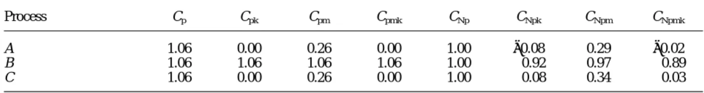
Table II. A comparison between Cp(u,v) and CNp(u,v)

Process Cp Cpk Cpm Cpmk CNp CNpk CNpm CNpmk

A 1.06 0.00 0.26 0.00 1.00 −0.08 0.29 −0.02

B 1.06 1.06 1.06 1.06 1.00 0.92 0.97 0.89

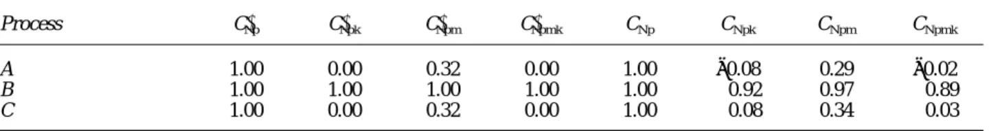
Table III. A comparison between CNp(u,v) and CNp(u,v)9

Process CNp9 CNpk9 CNpm9 CNpmk9 CNp CNpk CNpm CNpmk

A 1.00 0.00 0.32 0.00 1.00 −0.08 0.29 −0.02

B 1.00 1.00 1.00 1.00 1.00 0.92 0.97 0.89

C 1.00 0.00 0.32 0.00 1.00 0.08 0.34 0.03

obtain the percentile estimators for CNp(u,v), which in is the weight. For each model of rubber edges,

a unique production specification (USL, T, LSL) is may be expressed as the following:

set to the manufacturing processes. The weight of the rubber edge should not fall outside the

specifi-CˆNp(u,v)= d−uuMˆ−mu 3

!

F

F ˆ 99.865−F ˆ 0.135 6

G

2 + v(Mˆ−T)2

, (5) _{cation intervals or the customers will not accept} the products.

In the rubber-edge manufacturing factory, the raw rubber is first compounded through the kneader with

Fˆ99.865=X(R₁)+

SF

99.865n+0.135

100

G

−R1

D

some chemical powder. The compounded raw rubber is then cut into thin rubber strips with appropriate (X(R₁+1)−X(R₁)), (6) length, loaded onto the mold machines, and

thermo-casted into the desired shape of rubber edges. Differ-ent models of rubber edges have differDiffer-ent designs,

Fˆ0.135=X(R₂)+

SF

0.135n+99.865

100

G

−R2

D

shapes, weights, and have different production speci-fications. One characteristic of the rubber edge (X(R₂+ 1)−X(R₂)), (7)

which we studied was the weight. The upper and lower specification limits, USL and LSL, of the

Mˆ =X(R₃)+

SF

n+1

2

G

−R3

D

(X(R3+1)−X(R3)), (8) weight for a particular model of rubber edge, which

we studied, were set to 8.94 and 8.46 (in grams). The target value is the mid-point between the two where R1 = [(99.865n +0.135)/100], R2 =[(0.135n

specification limits, which is 8.70. The collected + 99.865)/100], R3 = [(n+1)/2]. In this setting, [R]

sample data (a total of 100 observations) are dis-is defined as the greatest integer less than or equal

played below in Table IV. to the number R, and X(i) is defined as the ith

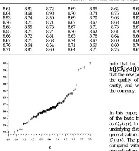
Figure 3 displays the normal probability plot for order statistic.

the collected data. We also perform Shapiro–Wilk test for normality check, obtaining W=0.91 with p-6. AN APPLICATION value=0.0001. Since the p-value is sufficiently small, we may conclude that the data set comes To illustrate how to calculate process capability

from a non-normal distribution. To calculate the using CNp(u,v), we consider the following example

values of the estimators CˆNp(u,v), we first calculate

taken from a company who is a manufacturer and

the sample percentiles obtaining Fˆ0.135=8.53,

supplier of speaker components (parts) supplying

Fˆ99.865=9.03, and M

ˆ

=8.69. Then, we substitute various kinds of rubber edges to speaker driver

these values into the definition of CˆNp(u,v) obtaining

manufacturing factories for making speaker driver

CˆNp=0.96, C

ˆ

Npk=0.92, C

ˆ

Npm=0.95, and

units. A standard (woofer) driver unit, as depicted

CˆNpmk=0.91. We note that CNpk value is less than

in Figure 2, consists of the following components

1.00, which indicates that the process is not adequate (parts) including edge, cone, dustcap, spider

with respect to the given manufacturing specifi-(damper), voice coil, lead wire, frame (basket),

cations, either the process variation (s2_{) needs to}

magnet, front plate, and back plate (T-york). The

be reduced or the process mean (m) needs to be rubber edge is one of the key components which

shifted closer to the target value. In fact, there are reflect sound quality of the driver units, such as

four observations (8.98, 8.99, 9.00, 9.03) falling musical image and clarity of the sound. One

charac-outside the specification interval (LSL, USL), and teristic of the rubber edge which we were interested

the proportion non-conforming is 4%.

The quality condition of such a process was con-sidered to be unsatisfactory in the company. Some quality improvement activities involving Taguchi’s parameter designs, were initiated to identify the significant factors causing the process failing to meet the company’s requirement. Consequently, machine settings for cutting the rubber strips as well as other process parameters were adjusted. To check whether the adjusted process was satisfactory, a new sample Figure 2. A speaker woofer driver of 100 from the adjusted process were collected

Table IV. 100 Observations of weight 8.61 8.81 8.72 8.69 8.65 8.64 8.68 8.74 8.68 8.67 8.64 8.68 8.98 8.70 8.74 8.75 8.66 9.00 8.64 8.70 8.53 8.74 8.59 8.69 8.70 9.03 8.83 8.87 8.79 8.68 8.76 8.71 8.71 8.67 8.67 8.68 8.69 8.74 8.80 8.59 8.68 8.55 8.73 8.67 8.71 8.73 8.67 8.68 8.69 8.74 8.55 8.71 8.74 8.70 8.62 8.61 8.79 8.69 8.68 8.77 8.66 8.72 8.81 8.63 8.78 8.64 8.66 8.63 8.71 8.99 8.67 8.71 8.63 8.74 8.67 8.69 8.69 8.68 8.70 8.81 8.76 8.64 8.54 8.71 8.69 8.80 8.70 8.59 8.53 8.74 8.71 8.81 8.60 8.64 8.71 8.75 8.67 8.73 8.61 8.84

note that for the new process the departure ratio

k=uT−mu/d=0.01 is quite small, which indicates that the new process is nearly on-target. As a result, the quality of the new process improved signifi-cantly, and was considered to be satisfactory in the company.

7. CONCLUSIONS

In this paper, we considered some generalizations of the basic indices Cp(u,v), which we referred to

as CNp(u,v), to cover non-normal distributions. If the

underlying distribution is normal, then the proposed generalizations CNp(u,v) reduce to the basic indices

Cp(u,v). The proposed generalizations CNp(u,v) are

compared with the basic indices Cp(u,v) and other

generalizations C9Np(u,v). The results indicated that

Figure 3. The normal probability plot for the collected datas

the proposed generalizations CNp(u,v) are more

(from the original process)

accurate than Cp(u,v) and CNp9(u,v) in measuring

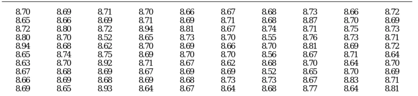
yielding the following measurements. Figure 4 dis- _{process capability.}

plays the normal probability plot for the collected _{In addition, we considered an estimation method} data presented in Table V. We perform Shapiro– _{based on sample percentiles to calculate CNp(u,v).} Wilk test for normality check, obtaining W=0.87 _{Computations for obtaining the estimators C}ˆ_Np(u,v) with p-value=0.0001. Since the p-value is suf- _{do not require any statistical tables, or any} assump-ficiently small, we conclude that the adjusted process _{tions on the underlying distributions. We also gave} is non-normal. We performed the same calculations _{an example on speaker components manufacturing} over the new sample of 100 observations. We _{process to illustrate how we apply the proposed} obtained the sample percentiles Fˆ0.135 = 8.52, F

ˆ

99.865 generalizations C_Np(u,v) to the actual data collected

=8.94, and Mˆ =8.69. Then, CˆNp=1.14, C

ˆ

Npk=1.10, from the factory. The calculations are easy to

under-CˆNpm=1.13, and C

ˆ

Npmk=1.08. We note that the stand, straightforward to apply, and should be

new (adjusted) process has zero defectives. We also _{encouraged for applications.}

acknowledgement

The authors thank the Chief Editor, Henry A. Malec, and the anonymous referees for their careful reading of the paper and several suggestions which improved the paper.

REFERENCES

1. V. E. Kane, ‘Process capability indices’, Journal of Quality

Technology, 18(1), 41–52 (1986).

2. L. K. Chan, S. W. Cheng and F. A. Spiring, ‘A new measure of process capability: Cpm’, Journal of Quality Technology,

20(3), 162–175 (1988).

3. W. L. Pearn, S. Kotz and N. L. Johnson, ‘Distributional and inferential properties of process capability indices’, Journal

of Quality Technology, 24(4), 216–233 (1992).

4. R. A. Boyles, ‘Process capability with asymmetric toler-ances’, Communications in Statistics—Simulation and Com-Figure 4. The normal probability plot for the collected datas

Table V. Second 100 Observations of weight 8.70 8.69 8.71 8.70 8.66 8.67 8.68 8.73 8.66 8.72 8.65 8.66 8.69 8.71 8.69 8.71 8.68 8.87 8.70 8.69 8.72 8.80 8.72 8.94 8.81 8.67 8.74 8.71 8.75 8.73 8.80 8.70 8.52 8.65 8.73 8.70 8.55 8.76 8.73 8.71 8.94 8.68 8.62 8.70 8.69 8.66 8.70 8.81 8.69 8.72 8.65 8.74 8.75 8.69 8.70 8.70 8.56 8.67 8.71 8.64 8.63 8.70 8.92 8.71 8.67 8.62 8.68 8.70 8.64 8.70 8.67 8.68 8.69 8.67 8.69 8.69 8.52 8.65 8.70 8.69 8.66 8.69 8.68 8.69 8.68 8.73 8.73 8.67 8.83 8.71 8.69 8.65 8.93 8.64 8.67 8.64 8.68 8.77 8.64 8.81

5. W. L. Pearn and K. S. Chen, ‘Estimating process capability 15. J. A. Clements, ‘Process capability calculations for non-normal distributions’, Quality Progress, September, pp. 95– indices for non-normal Pearsonian populations’, Quality &

Reliability Engineering International, 11(5), 386–388 (1995). 100 (1989).

16. G. F. Gruska, K. Mirkhani and L. R. Lamberson, Non normal 6. D. Zwick, ‘A hybrid method for fitting distributions to data

and its use in computing process capability indices’, Quality data analysis, Multiface Publishing Co, Michigan, 1989.

17. P. L. Chang and K. H. Lu, ‘PCI calculations for any shape of

Engineering, 7(3), 601–613 (1995).

7. Y. M. Chou, D. B. Owen and S. A. Borrego, ‘Lower distribution with percentile’, Quality World, technical section (September), 110–114 (1994).

confidence limits on process capability indices’, Journal of

Quality Technology, 22(3), 223–229 (1990).

8. S. Kotz, W. L. Pearn and N. L. Johnson, ‘Some process

capability indices are more reliable than one might think’, _{Authors’ biographies:}

Journal of the Royal Statistical Society, Series C: Applied

Statistics, 42(1), 55–62 (1993). _{K. S. Chen received his M.S. in Statistics from National}

9. K. Va¨nnman, ‘A unified approach to capability indices’,

Cheng Kung University, and Ph.D. in Quality Control

Statistica Sinica, 5, 805–820 (1995).

from National Chiao Tung University. Currently, he is an

10. W. L. Pearn and K. S. Chen, ‘A Bayesian-like estimator of

associate professor in Department of Industial Engineering

Cpk’, Communications in Statistics: Simulation &

Compu-and Management, National Chin-Yi Institute of

Tech-tation, 25(2), 321–329 (1996).

11. L. K. Chan, S. W. Cheng and F. A. Spiring, ‘The robustness nology, Taichung, Taiwan, R.O.C.

of the process capability index Cp, to departures from

nor-mality’, Statistical Theorey and Data Analysis II (edited by _{W. L. Pearn is a professor of operations research and} K. Matusita), pp. 223–239, North Holland, 1988. _{quality management in Department of Industrial} Engineer-12. B. H. Gunter, ‘The use and abuse of Cpk. Part 3’, Quality _{ing & Management, National Chiao Tung University,}

Tai-Progress, May, 79–80 (1989).

wan, R.O.C. He received his M.S. in statistics, and Ph.D.

13. Somerville, S. E. and Montgomery, D. C. ‘Process capability

in operations research from the University of Maryland at

indices and non-normal distributions’, Quality Engineering,

College Park, MD, U.S.A. He worked for AT&T Bell

9(2), 305–316 (1997).

Laboratories at Switch Network Control Center as a

Sys-14. H. Schneider, J. Pruett and C. Lagrange, ‘Uses of process

tem Engineer, and Process Quality Center as a Quality

capability indices in the supplier certification process’,