順滑模態理論應用於有限元素法模式之撓性臂控制

國 立 交 通 大 學

電 機 與 控 制 工 程 學 系

碩 士 論 文

順滑模態理論應用於有限元素法模式之

撓性臂控制

Sliding Mode Theory Applied to the control

of FEM-based Flexible Arm

研 究 生：張 人 中

指導教授：陳 永 平 教授

順滑模態理論應用於有限元素法模式之

撓性臂控制

Sliding Mode Theory Applied to the control

of FEM-based Flexible Arm

研 究 生：張 人 中

Student：Jen-Chung Chang

指導教授：陳永平 博士 Advisor：Dr. Yon-Ping Chen

國 立 交 通 大 學

電機與控制工程學系

碩士論文

A Thesis

Submitted to Department of Electrical and Control Engineering

College of Electrical and Computer Engineering

National Chiao Tung University

In Partial Fulfillment of the Requirements

For the degree of Master

In

Electrical and Control Engineering

June 2006

Hsinchu, Taiwan, Republic of China

順滑模態理論應用於有限元素法模式之

撓性臂控制

學生：張 人 中

指導教授：陳永平 博士

　

國立交通大學電機與控制工程學系

摘 要

在本篇論文中，我們研究如何穩健控制撓性臂頂端位置的問

題。首先以有限元素法推導撓性臂的數學模型，將非線性的撓性

臂的高階模式省略，求出一個近似的線性數學模型。而這些被省

略的高階撓性臂模式，與系統結構的不確定項一起當成系統外在

的擾亂。知名的穩健順滑模式理論可以對付這些擾亂，做有效的

控制。模擬以及實驗的結果顯示順滑控制理論的穩健以及在控制

結果上的優越。

Sliding Mode Theory Applied to the control

of FEM-based Flexible Arm

Student:

Jen-Chung Chang

Advisor:

Dr.

Yon-Ping

Chen

Department of Electrical and Control Engineering

National Chiao Tung University

ABSTRACT

This thesis studies the robust problem of the tip position control of a physical flexible arm. Its linear model is mathematically derived by the finite element method (FEM), which is approximate to the nonlinear flexible arm by neglecting the higher order modes. As a result, these higher order modes are considered as the disturbances of the linear model of the flexible arm. In addition, uncertainties subject to the structure and payload variations are also included in the linear model. To cope with these disturbances and uncertainties, the well-known robust control technique, the sliding-mode control, is employed to effectively control the tip position of the flexible arm. Finally, simulation and experimental results are used to demonstrate the robustness and superiority of the sliding mode control.

Acknowledgement

首先要對指導教授 陳永平教授至上最高的敬意，對於我研究方面的指 導與英文寫作表達上的督促，使我這兩年來成長收穫許多。還有可變結構 實驗室的桓展，克聰，建峰，豐洲，世宏學長，及宜穎，思穎，仲賢以及 學弟妹們在研究所兩年歲月裡的陪伴，無論是研究課業上的分享討論，或 是研究之餘的互相鼓勵打氣，都讓我擁有最棒的研究環境和心情。 最後要特別感謝的是我的父母，以及弟弟，感謝你們對我的支持與關 心，謝謝你們，沒有你們就沒有這篇論文。 僅以此論文獻給所有關心，照顧我的親朋好友們。 張人中 6.16.2006

Contents

Chinese Abstract ……….i

English Abstract ……….ii

Acknowledgement …………..……….iii

Contents ……….iv

List of Figures……….vi

List of Tables ……….ix

Notations ………x

Chapter 1 Introduction 1.1 Preliminary ……….1

1.2 Content Organization….……….…….2

Chapter 2 System Modeling of a Flexible Arm 2.1 Introduction ………3

2.2 FEM-Based Model Description ………4

2.3 Nature Frequency Analysis of the Flexible Arm ………...12

2.4 Parameter Identification ………...14

Chapter 3 Controller Design 3.1 Introduction ………...19

3.2 Rigid Controller Design ………19

3.3 Introduction to the Variable Structure Control (VSC) ………..20

3.4 Sliding Mode Controller Design ………..22

Chapter 4 Simulation Results 4.1 Pole Placement ……….28

Chapter 5 Experimental Demonstration

5.1 Experimental Setup ………..34

5.1.1 Matlab xPC Target Environment ………..34

5.1.2 Motor Setup ………..36

5.1.3 Deflection Measurement ………..37

5.2 Sliding Mode Controller Experimental Results ………..43

5.3 Experimental Results of Impulse Disturbance ……….52

5.4 Experimental Results with Tip-Mass Loading ………58

Chapter 6 Conclusions ………66

Reference ………..67

Appendix A Local mass matrix and stiffness matrix ………69

Appendix B Measurement of Young’s Module ……….71

List of Figures

Fig. 2.2.1 The flexible arm structure ………5

Fig. 2.2.2 Four degrees of freedom ofan element ………..8

Fig. 2.2.3 Shape functions ………9

Fig. 2.4.1 Experimental plant ……….14

Fig. 2.4.2 (a) Coupled model frequency response………..17

Fig. 2.4.2 (b) Uncoupled model frequency response ……….18

Fig. 3.3.1 Sliding Mode Control input combined with different inputs ………….21

Fig. 3.4.1 Sgn(s) function ……….25

Fig. 3.4.2 Sat(s) function ………..26

Fig. 4.1.1The system poles of the flexible arm ……….29

Fig. 4.1.2The desired poles of the sliding mode controller ………30

Fig. 4.2.1 Hub angle regulation in sliding mode control ………..31

Fig. 4.2.2 Four states response in sliding mode control ………....31

Fig. 4.2.3 Sliding surface in sliding mode control ………..32

Fig. 4.2.4 Norm of the error states in sliding mode control ………...32

Fig. 4.2.5 Tip position regulation in sliding mode control ………33

Fig. 5.1.1 Hardware Architecture ………..35

Fig.5.1.2 Wheatstone Bridge Circuit ……….38

Fig.5.1.3 Voltage Amplifier Circuit ………39

Fig.5.1.4 Low Pass Filter Circuit ………..40

Fig.5.1.5 Low Pass Filter Bode Plot ……….40

Fig. 5.2.1 Hub angle regulation in rigid control ………44

Fig. 5.2.3 Four states response in rigid control ……….45

Fig. 5.2.4 Hub angle regulation in SMC (ε =0.01 andσ =5) ……….46

Fig. 5.2.5 Tip position regulation in SMC (ε =0.01andσ =5) ...46

Fig. 5.2.6 Four states response in SMC (ε =0.01andσ =5) ………...47

Fig. 5.2.7 Sliding surface in SMC (ε =0.01andσ =5) ……….47

Fig. 5.2.8 Hub angle regulation in SMC (ε =0.0067andσ =6) ………..48

Fig. 5.2.9 Tip position regulation in SMC (ε =0.0067andσ =6) ………...48

Fig. 5.2.10 Four states response in SMC (ε =0.0067andσ =6) ………..49

Fig. 5.2.11 Sliding surface in SMC (ε =0.0067andσ =6) ………..49

Fig. 5.2.12 Hub angle regulation in SMC (ε =0.005andσ =8) ………50

Fig. 5.2.13 Tip position regulation in SMC (ε =0.005andσ =8) …….…….50

Fig. 5.2.14 Four states response in SMC (ε =0.005andσ =8) ...51

Fig. 5.2.15 Sliding surface in SMC (ε =0.005andσ =8) ……….…….51

Fig. 5.3.1 Hub angle response in rigid control ……….53

Fig. 5.3.2 Tip position response in rigid control ……….……….54

Fig. 5.3.3 Four states response in rigid control ……….…………54

Fig. 5.3.4 Frequency response of vibration in rigid control ………..55

Fig. 5.3.5 Hub angle response in sliding mode control ……….……...56

Fig. 5.3.7 Four states response in sliding mode control ………..…………57

Fig. 5.3.8 Sliding surface in sliding mode control ………57

Fig. 5.3.9 Frequency response of vibration in sliding mode control ……….58

Fig. 5.4.1 Hub angle regulation in rigid control (m_t =0.102kg) ………59

Fig. 5.4.2 Tip position regulation in rigid control (m_t =0.102kg) ……….60

Fig. 5.4.3 Four states response in rigid control (m_t =0.102kg) ………..60

Fig. 5.4.4 Hub angle in SMC (m_t =0.102kg, ε =0.01andσ =6) ……….61

Fig. 5.4.5 Tip position in SMC (m_t =0.102kg, ε =0.01andσ =6) ………….61

Fig. 5.4.6 Four states response in SMC (m_t =0.102kg, ε =0.01andσ =6) ….62 Fig. 5.4.7 Sliding surface in SMC (m_t =0.102kg, ε =0.01andσ =6) ………62

Fig. 5.4.8 Hub angle in SMC (m_t =0.102kg, ε =0.005andσ = 7) …………63

Fig. 5.4.5 Tip position in SMC (m_t =0.102kg, ε =0.005andσ = 7) ………..63

Fig. 5.4.6 Four states response in SMC (m_t =0.102kg, ε =0.005andσ =7) .64 Fig. 5.4.7 Sliding surface in SMC (m_t =0.102kg, ε =0.005andσ = 7) …….64

List of Tables

Table 2.4.1: Physical parameters of the system ……….15 Table 2.4.2: Nature frequencies (Hz) of coupled and uncoupled models ………..17 Table 5.1.2 Servo Motor Specifications ……….………..36

Notations

A,B,C : Upper-case bold italic letters denote matrices. a,b,c : Lower-case bold italic letters denote vectors.

a,b,c : Lower-case italic letters denote scalars. w : Deformation of beam.

θ : Rotary angle of hub. ρ : mass per unit length.

E : Young’s modulus of elasticity.

I : area moment of inertia of the arm’s cross section.

Jh : Rotary inertia of hub. u : Input torque.

( )

⋅

φ : Shape function for beam.

s : Sliding surface.

( )

⋅

sgn : The sign function. sat

( )

⋅ : The saturation function.

Chapter 1

Introduction

1.1 Preliminary

Recently, the control problems of flexible systems have been intensively studied

due to the challenging demand of fast and precise manipulators in various industrial

and space applications. In future space applications, the manipulators will need to be

lighter and to move faster with higher accuracy. The reduced inertias of these lighter

and faster manipulators unavoidably result in vibration. Thus, it is important to

investigate the dynamics and control problems for manipulators with structure

flexibility. The desired control strategy for the flexible arms is not only to control the

motion of the rigid mode with reasonable accuracy, but also to suppress the vibration

of the arm to achieve high speed and precise tip position.

Since the tip position motion of the lightweight flexible arm has an infinite

number of modes, most of the investigators [1, 2, 14, 18] adopt the so-called finite

freedom model to simulate the real flexible arm. Instead, this thesis uses the finite

element method (FEM) to derive a reduced-order model for the flexible arm.

controlling uncertain systems [3]. Besides, the sliding mode control for flexible arms

has been widely studied [2, 16, 17, 18]. In these papers, numerical simulation results

show that the flexible arm is effectively controlled by SMC. In this thesis, an

experimental flexible arm is set up to control the flexible arm tip position. In addition,

the robustness of the proposed sliding mode controller is compared with the rigid

controller by applying impulse disturbance and payload variation to the flexible arm.

1.2 Content Organization

This thesis is organized into six chapters. Chapter 1 gives an introduction.

Chapter 2 describes the FEM model of the flexible arm. Chapter 3 presents the

scheme and theorem of sliding mode controller. The control purpose in this thesis is to

regulate the hub angle of the flexible arm with vibration suppressed. Chapter 4

simulates the flexible arm control in Matlab and then Chapter 5 fulfills the experiment.

Chapter 2

System Modeling of a Flexible Arm

Although there are some documents using system identification method to

identify the flexible arm model [19], the derived mathematical model is used in this

thesis because of its accuracy of physical meaning to describe the nonlinear model.

2.1 Introduction

Mathematical model derivation of flexible arm is generally concluded into two

methods. One is using Assumed Mode Method (AMM), and the other is using Finite

Element Method (FEM). In Assumed Mode Method, the vibration modes in flexible

arm are considered as shape functions, and the amplitude of these modes are state

variables. The shape function of AMM is more complicated and could not be used for

different complex geometry shape system. It means that different plant needs different

shape function. FEM divides the flexible arm into several elements, and the shape

function of each one is the same. The shape functions are simple polynomial

equations and do not change when different complex geometry shape flexible arm is

easier to get from the strain gauge feedbacks. The FEM-based flexible arm model is

derived as follows.

A clamped-free single flexible arm is generally modeled by a partial differential equation [9], expressed as

p t w ρ x w EI x 2 2 = ∂ ∂ + ⎟⎟ ⎠ ⎞ ⎜⎜ ⎝ ⎛ ∂ ∂ ∂ ∂ 2 2 2 2 (2.1.1) where

E : Young’s modulus of elasticity.

I : area moment of inertia of the arm’s cross section. w : transverse displacement (deformation).

ρ: mass per unit length.

p : external force per unit length.

There is no exact solution for (2.1.1). Instead, an approximate approach using polynomials is adopted to solve the partial differential equation. A more correct solution will be obtained when higher order polynomials are used. FEM is employed to derive the single flexible arm model in this paper.

2.2 FEM-Based Model description

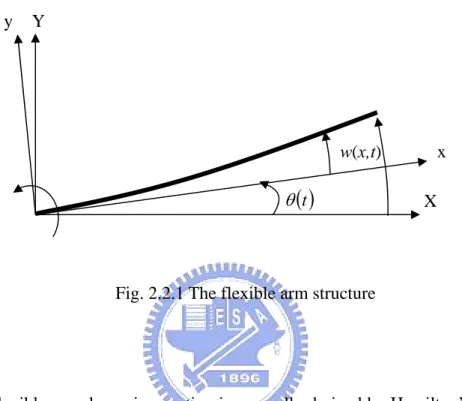
The flexible arm is a one-meter stainless steel ruler shown in Fig. 2.2.1. The left-hand side of the arm is clamped on the motor joint and the right-hand side is free. Consider vibration and rotation in horizontal direction and neglect shear deformation, as in the Euler-Bernoulli beam shown in Fig. 2.2.1. The motor rotational angleθ

( )

t and deformation, transverse displacement, w , are expressed in the fixed X-Y

( )

x t

coordinate system and reference x-y coordinate system, respectively. To model the FEM structure, it is required that the transverse displacement w , be small, less

( )

x t than one tenth of the full arm length.

y Y

w(x,t) x

( )

t

θ X

Fig. 2.2.1 The flexible arm structure

The flexible arm dynamic equation is generally derived by Hamilton’s principle

described as

(

)

2 0 1 2 1 = + −

∫

∫

t t nc t t δ T V dt δW dt (2.2.1) where

T : system kinetic energy V : system potential energy

nc

W

δ : virtual work by non-conservative forces

The system kinetic energy is composed of rotational and moving energies, written as

( )

+

_∫

( )

= L 0 2 2 h ρv x,t dx 2 1 t θ J 2 1 T & (2.2.2)

v=v

( ) ( ) (

x,t =w& x,t + x+r

) ( )

θ&t represents flexible arm velocity.

Because the flexible arm rotates on the horizontal plane, the gravity potential energy is neglected, and total system potential energy only contains strain energy, expressed by

∫

⎜⎜_⎝⎛∂_∂ ⎟⎟_⎠⎞ = L dx x w EI V 0 2 2 2 2 1 (2.2.3)

Virtual work δW_nc done by non-conservative force is described as

( )

t u W_nc δθ

δ = ₁ (2.2.4)

where u1 is the motor torque applied to the system. Substituting T, V and δWnc into

(2.2.1) yields

(

)

(

)

(

(

)

)

0 2 1 = ⎥ ⎦ ⎤ ⎢ ⎣ ⎡ + + ⎟⎟ ⎠ ⎞ ⎜⎜ ⎝ ⎛ ∂ ∂ ⎟⎟ ⎠ ⎞ ⎜⎜ ⎝ ⎛ ∂ ∂ − + + + +

∫ ∫

∫

dx J θδθ u δθ dt x w δ x w EI dx θ δ r x w δ θ r x w ρ L 0 L 0 2 h 1 2 2 2 t

t & & & & & &

(2.2.5)

From the truth of

∫

∫

⎟⎟ ⎠ ⎞ ⎜⎜ ⎝ ⎛ ∂ ∂ − ∂ ∂ = ∂ ∂ 2 1 2 1 2 1 t t i i t t i i t t i i dt q q T dt d q q T dt q q T _{δ δ δ} & & & & (2.2.6)

and the assumption of δq_i

( )

t₁ =δq_i

( )

t₂ =0 in Hamilton’s principle, we have

∫

∫

⎟⎟ ⎠ ⎞ ⎜⎜ ⎝ ⎛ ∂ ∂ − = ∂ ∂ 2 1 2 1 t t i i t t i i dt δq q T dt d dt q δ q T & & & and rearrange (2.2.5) as

(

)

(

)

(

x r

) (

(

w x r

)

θ

)

dx J θ u δθ dt 0 ρ dx x w δ x w EI δw θ r x w ρ L 0 h 1 t t L 0 2 2 2 2 2 1 = ⎭ ⎬ ⎫ ⎥⎦ ⎤ ⎢⎣ ⎡ _{+ + + + −} + ⎪⎩ ⎪ ⎨ ⎧ ⎥ ⎦ ⎤ ⎢ ⎣ ⎡ ⎟⎟ ⎠ ⎞ ⎜⎜ ⎝ ⎛ ∂ ∂ ⎟⎟ ⎠ ⎞ ⎜⎜ ⎝ ⎛ ∂ ∂ + + +

∫

∫ ∫

&& && && && && (2.2.7)

where is the deformation that refers to the rotational reference coordinate

system x-y and is described by FEM. Since and

(

x t w ,

)

dx δθ are linear independent, we

have

(

)

(

)

∫

_⎥ = ⎦ ⎤ ⎢ ⎣ ⎡ ⎟⎟ ⎠ ⎞ ⎜⎜ ⎝ ⎛ ∂ ∂ ⎟⎟ ⎠ ⎞ ⎜⎜ ⎝ ⎛ ∂ ∂ + + + L dx x w x w EI w r x w 0 2 2 2 2 0 δ δ θ ρ _&& && (2.2.8)

(

)

(

(

)

)

0 0 1⎥⎦ = ⎤ ⎢⎣ ⎡

_∫

L_{ρ + + + θ + θ− δθ} h u J dx r x w r

x _&& && && (2.2.9)

Based on FEM, the flexible arm consists of many linear piecewise arm elements, each

with four degrees of freedom (DOF). The deformation w , of the j-th element is

( )

x t written as

( )

(

)

( )

1 4 1 + = < < − =

∑

_{j j} i ij j i x x v t x x x t x, w φ (2.2.10)

where v1j(t) and v2 j(t) (v3j(t) and v4j(t)) represent the transverse deflection and rotation

at node j (j+1) as depicted in Fig. 2.2.2, and φ_i

( )

x means the shape functions [6]. To solve the shape functions φ_i

( )

x , i=1,2,3,4, the following boundary conditions must be satisfied

( )

( )

( )

( )

(

)

( )

(

x t,

)

v

( )

t w t t v t, x w t v t, x w t t v t, x w j 4 j j 3 j j 2 j j 1 j = ∂ ∂ = = ∂ ∂ = + + 1 1 (2.2.11)

Fig. 2.2.2 Four degrees of freedom ofan element

Substituting (2.2.11) into (2.2.10) yields

( )

0 =1 1 φ , φ&1

( )

0 =φ1

( )

h =φ&1

( )

h =0 2

( )

0 =1 φ& , φ2

( )

0 =φ2

( )

h =φ&2

( )

h =0

( )

1 3 h = φ , φ₃

( )

0 =φ&₃

( )

0 =φ&₃

( )

h =0

( )

h =1 φ&₄ , φ4

( )

0 =φ&4

( )

0 =φ4

( )

h =0 (2.2.12)

where h is the length of the flexible arm. Since there are four boundary conditions per

interpolation function, the simplest functions we can select are linear polynomials of

the form

( )

_x =_C +_{C x}+_{C x}2+_{C x}3

Substitute (2.2.12) into (2.2.13) to solve the four shape functions, which are obtained as

( )

( )

(

)

( )

( )

1 + < < ⎟⎟ ⎠ ⎞ ⎜⎜ ⎝ ⎛ − + ⎟⎟ ⎠ ⎞ ⎜⎜ ⎝ ⎛ − − = ⎟⎟ ⎠ ⎞ ⎜⎜ ⎝ ⎛ − − ⎟⎟ ⎠ ⎞ ⎜⎜ ⎝ ⎛ − = ⎟⎟ ⎠ ⎞ ⎜⎜ ⎝ ⎛ − + ⎟⎟ ⎠ ⎞ ⎜⎜ ⎝ ⎛ − − − = ⎟⎟ ⎠ ⎞ ⎜⎜ ⎝ ⎛ − + ⎟⎟ ⎠ ⎞ ⎜⎜ ⎝ ⎛ − − = j j 3 j 2 j 4 3 j 2 j 3 3 j 2 j j 2 3 j 2 j 1 x x x h x x h h x x h x φ h x x 2 h x x 3 x φ h x x h h x x h 2 x x x φ h x x 2 h x x 3 1 x φ (2.2.14)

where x is the distance to the base.

Fig. 2.2.3 Shape functions

Calculate the second partial derivative of w , to time and the second partial

( )

x t derivative of w ,

(

x t

)

_{to x, then}

)

( )

_∑

( ) (

= = 4 1 i ij i x v t t, x w_&& φ _&& (2.2.15)

( )

_∑

_[

_{( )}

_]

_{( )}

= ∂ ∂ = ∂ ∂ 4 1 2 2 2 2 i ij i x v t x x t, x w φ (2.2.16)

Substituting (2.2.15) and (2.2.16) into (2.2.8) and (2.2.9) and integrating spatial

domains leads to the global mass and stiffness matrices (the local mass and stiffness

matrices are showed in Appendix A). The assembled set of matrix differential

equations is as follows [1, 2, 14, 18]: u N b x x+ K = M && (2.2.17) where

N is the number of elements,

⎥ ⎦ ⎤ ⎢ ⎣ ⎡ = v x θ where

[

]

T N N v v v v1 2 2 −1 2 = _L v

represents the state variables,

⎥ ⎦ ⎤ ⎢ ⎣ ⎡ = 0 1 N

b represents the single input, and

⎥ ⎦ ⎤ ⎢ ⎣ ⎡ + = vv vθ θv M M M M Jh Mθθ

represents the mass matrix for the FEM-based model.

⎥ ⎦ ⎤ ⎢ ⎣ ⎡ = vv K 0 0 0

K represents the stiffness matrix for the FEM-based model.

where

∑

= = N i i 1 11 M θθ M M_θv =M_vθT =

[

M₁₃1 +M₁₂2 M₁₃2+M₁₂3 M₁₃3 +M₁₂4 _L M₁₃N−1+M₁₂N−1 M₁₃N

]

⎥ ⎥ ⎥ ⎥ ⎥ ⎥ ⎥ ⎥ ⎦ ⎤ ⎢ ⎢ ⎢ ⎢ ⎢ ⎢ ⎢ ⎢ ⎣ ⎡ + + + + = − − N 33 N 32 N 23 N 22 1 N 33 1 N 32 4 23 4 22 3 33 3 32 2 23 3 22 2 33 2 32 2 23 2 22 1 33 vv M M M M M M M M M M M M M M M M M M O where

(

) (

)(

) (

)

[

2 2

]

11 3 x r x r h x r x r h h i i i i i ₌ ρ _{+ + + + + + + +} M

(

)

(

)

_⎥⎦⎤ ⎢⎣ ⎡ _{+ + + +} = = h h x_i r h x_i r 12 1 30 1 2 1 20 3 2 ρ T i 21 i 12 M M

(

)

(

)

_⎥⎦⎤ ⎢⎣ ⎡ _{+ +} − _{− +} = = h h x_i r h h x_i r 12 20 1 2 1 20 7 2 ρ T i 31 i 13 M M ⎥ ⎦ ⎤ ⎢ ⎣ ⎡ = ₂ 4 22 22 156 420 h h h h Mi ρ 22 ⎥ ⎦ ⎤ ⎢ ⎣ ⎡ − − = = ₂ 3 13 13 54 420 h h h h ρ T i 32 i 23 M M ⎥ ⎦ ⎤ ⎢ ⎣ ⎡ − − = ₂ 4 22 22 156 420 h h h ρh i 33 M , and ⎥ ⎥ ⎥ ⎥ ⎥ ⎥ ⎥ ⎥ ⎦ ⎤ ⎢ ⎢ ⎢ ⎢ ⎢ ⎢ ⎢ ⎢ ⎣ ⎡ + + + + = − − N 33 N 32 N 23 N 22 1 N 33 1 N 32 4 23 4 22 3 33 3 32 2 23 3 22 2 33 2 32 2 23 2 22 1 33 vv K K K K K K K K K K K K K K K K K K O where ⎥ ⎦ ⎤ ⎢ ⎣ ⎡ = _{3 2} 4 6 6 12 h h h h EI i 22 K ⎥ ⎦ ⎤ ⎢ ⎣ ⎡ − − = = _{3 2} 2 6 6 12 h h h h EI T i 32 i 23 K K ⎥ ⎦ ⎤ ⎢ ⎣ ⎡ − − = _{3 2} 4 6 6 12 h h h h EI i 33 K

Finally, the tip position defined as [8]

( )

x t L

( ) (

t w x t

t , = θ + ,

)

is also an important index in this thesis.

2.3 Nature frequencies of the flexible arm

To determine the nature frequencies of the flexible arm described in (2.2.17), the

inertial matrix M is often changed into MU by neglecting the coupling elements

between hub coordinate θ and flexible coordinates such that the dynamic equation

becomes as

(2.3.1)

u K

M_U x_&&+ x=b_N

where denotes the uncoupled inertial matrix. Hence, (2.3.1)

can be further decomposed into the following equations

⎥ ⎦ ⎤ ⎢ ⎣ ⎡ + = VV U M 0 0 M Jh Mθθ (2.3.2)

(

J_h+M_θθ

)

θ&&=u 0 (2.3.3) = +K v v M_{VV && VV}

Furthermore, the matrices M_VV and K_VV are symmetric and positive-definite.

N N U Λ U Λ U Λ Λ U ΛU U M 2 T 1 T 2 1 2 1 2 1 T T VV ⎟⎟= ⎠ ⎞ ⎜ ⎜ ⎝ ⎛ ⎟ ⎟ ⎠ ⎞ ⎜ ⎜ ⎝ ⎛ = = = (2.3.4)

where U is the orthogonal matrix, Λ is the diagonal matrix, and N Λ2U

1

(2.3.4), rewrite (2.3.3) into

Nv&&+K_VNNv=0 (2.3.5)

where K_VN = N−TK_VVN−1. It can be found that

(

N x

)

K

(

N x

)

y K y x N K N x x K x 1 T _VV VV T 1 1 VV T T VN T ₌ − − ₌ − − ₌ (2.3.6)

Which implies KVN is symmetric and positive definite, same as KVV. Hence, it can be

written as (2.3.7) ΩP P K T VN =

where P is the orthogonal matrix and is the diagonal matrix. Substituting (2.3.7)

into (2.3.5) yields Ω (2.3.8) 0 ΩPNv P v N + T = && 0 ΩPNv v PN&&+ =

Define a new modified state vector

, (2.3.9)

PNv y =

where y is the vetor of model coordinates. The transformed equation of

motion (2.3.3) becomes 1 2n× (2.3.10) 0 Ωy y&&+ = where (2.3.11) ⎥ ⎥ ⎥ ⎥ ⎥ ⎦ ⎤ ⎢ ⎢ ⎢ ⎢ ⎢ ⎣ ⎡ = ⎥ ⎥ ⎥ ⎥ ⎦ ⎤ ⎢ ⎢ ⎢ ⎢ ⎣ ⎡ = 2 2 2 2 2 1 2 2 1 0 0 0 0 0 0 0 0 0 0 0 0 0 0 0 0 n n w w w L M O M L L M O M L λ λ λ Ω

2.4 Parameter Identification

In order to test and validate the controller designed in this thesis, an experimental

setup, which is shown in Fig. 2.4.1, was developed.

Fig. 2.4.1 Experimental plant

Table 2.4.1: Physical parameters of the system

Arm length l 0.94[m]

Arm width 0.031[m]

Arm thick 0.0015[m]

Arm mass m 0.3706[kg] Flexible arm mass per unit length ρ 0.3554[kg/m]

Young’s modulus E 2.08×1011[Nt/m2] Cross-section inertia momentum I 8.718×10-12[m4] Hub rotary inertia Jh 1.12×10-4[kg m2]

Hub radius r 0.0265[m]

In Section 2.3, the nature frequencies of the flexible arm, shown in (2.3.12), are

derived for its uncoupled model. The Young’s modulus E could be determined from

the expression of nature frequencies of the uncoupled model (shown in Appendix B)

[17], which is constructed with the flexible arm fixed in the hub. To attain the nature

frequencies, an impulse force is generally required as the excitation source. In this

experiment, the impulse force is created by a hammer knocking near the root of the

flexible arm. After a knock, the strain gage feedback signal of the uncoupled flexible

arm is recorded. In order to get the nature frequencies of the uncoupled flexible arm,

a Fast Fourier transform (FFT) is performed for the signal to get the primary nature

frequencies which results in high amplitude response at the frequencies. For the

precise position of the nature frequencies, it is necessary to obtain many samples from

modulus E is derived in Appendix B. Since the Young’s modulus E is acquired, the

precise nature frequencies of the coupled model can be derived in the same way like

the derivation of section 2.3. The difference of the coupled model and the uncoupled

model is that the latter is neglecting the coupling elements between hub coordinate θ

and flexible coordinates. Because the controller is designed for the flexible arm FEM

model, it is important to make sure the accuracy of the FEM model. It is a good way

to check the accuracy of the FEM model by checking the nature frequencies of the

derived FEM model is the same as the experiment flexible arm. So, let the flexible

arm free with the hub and give a knock to the arm, the nature frequency response of

the coupled model is obtained by performing FFT to the strain gages feedback signal.

Finally, compare the nature frequencies of the coupled experimental model with the

derived model, the result, Table 2.4.2, shows that they were remarkably close to each

other, and it means that the finite-element-method is valid to describe the flexible arm

Table 2.4.2: Nature frequencies (Hz) of coupled and uncoupled models

Coupled Model Uncoupled model

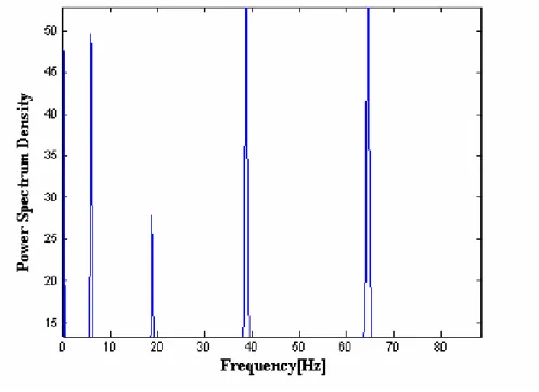
Fig. 2.4.2 shows the frequency response of coupled model and uncoupled model.

Fig. 2.4.2 (a) Coupled model frequency response

FEMb FEM Expa Nature freq. Exp N=2 N=10 N=40 N=2 N=10 N=40 f1 5.9 5.9404 5.9057 5.9056 1.5 1.4313 1.4306 1.4306 f2 18.8 20.474 18.918 18.916 8.9 9.0416 8.9658 8.9655 a

Exp means the experimental nature frequencies

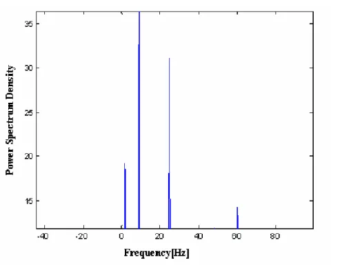
b

Fig. 2.4.2 (b) Uncoupled model frequency response

With the accurate flexible arm FEM model, the controller could be validly

Chapter 3

Controller Design

3.1 Introduction

Two main classes of controllers were considered here to control the hub angle of

the arm. Firstly, the flexible arm was modeled with a two-element FEM model

derived in Chapter 2, and a rigid controller was developed. Then, a sliding mode

controller was developed and its performance was compared with that of rigid

controller. These controllers were designed to meet the following specifications:

In response to a step inputs:

1. The steady-state error must be minimized.

2. The settling time must be minimized.

3. The vibration effect of the flexible arm hub angel and tip position must be

minimized.

3.2 Rigid Controller Design

so the coupled terms in the FEM model, the stiffness matrix, and the mass matrix

could be neglected. Then, the model is in a simple form:

(

J_R+M_θθ

)

θ&&=u (3.2.1)

In order to control such a double differential model, the PID controller is a candidate.

There are several well documented methods available to design PID controller.

Furthermore, PID controllers are relatively easy to implement. But in practical

Integral controller is not useful because that it may windup when the steady-state

error is large and may cause damage to the transient response, such as more overshoot

or undershoot. In this experiment, the drawback of I controller was verified, so PD

controller was adapted. In order to design a suitable PD controller for the flexible arm,

the PD parameters are chosen based on the FEM model. From (3.2.1),

(

JR +M_θθ

)

θ&&=u=kDθ&+kPθ (3.2.2)

Then, the poles placement method was used to assign the two poles to the left half

plane in s domain. Because the motor has limited maximum torque, the two poles

should be assigned to the proper position for the purpose that the input could be below

the maximum value.

Variable structure control (VSC) is one influential method to deal with the

uncertainties of system. The structure of a VSC is a nonlinear control that switches

with different control input, according to some pre-assigned algorithm or law of

substructure change in the current value of the error signal and its derivatives. For

example, assume there is a system

u x x&&+ = With its initial condition,

( )

0 =1 x

( )

0 =0 x &

VSC is used to changing the input u in different conditions in fig.3.3.1. The response

of x is better than the conditional control because VSC combines the advantages of

the different inputs.

0 2 4 6 8 10 12 14 16 18 20 -1 -0.8 -0.6 -0.4 -0.2 0 0.2 0.4 0.6 0.8 1 time(sec) x sliding-mode control line u=-5x ---- u=0 xxxx u=0 when x>0.05 u=-5x when x<=0.05

Sliding mode control is an influential control method and is generally chosen for

VSC nowadays. At first, a stable sliding surface should be determined in sliding mode

control. The state variables of the system will lead to the sliding surface by variable

structure control and will not leave the sliding surface. VSC is robust for the noise and

disturbance and its rise time and transient response are also satisfied. Generally there

are two steps in designing the sliding mode controller, the first is choosing the sliding

surface, and the second is designing the sliding mode controller. The purpose of the

second one is to reaching the sliding surface in limited time and it is easier to achieve

than the first. Choosing a good sliding surface is an art.

3.4 Sliding Mode Controller Design

The purpose of this experiment is to rotate the flexible arm to the desired angle

d

θ and eliminate the vibration of the arm. So the state variables of the FEM should

be brought to zero finally, in the beginning, the controllability of the plant model must

be checked out. From (2.2.17), because M is positive definite matrix that its inverse

matrix is exist.

Bu Ax

x_& = + (3.4.1)

⎥ ⎦ ⎤ ⎢ ⎣ ⎡ − = ₋ 0 K M I 0 A ₁ (3.4.3) ⎥ ⎦ ⎤ ⎢ ⎣ ⎡ = ₋ N b M 1 0 B (3.4.4)

PBH test shows that

(

A,B

)

is controllable if and only if rank

(

λI−A B

)

is full rank for all eigenvalues λ . After checking all the eigenvalues, the result shows that

the flexible arm FEM model is controllable and could be used poles placement

method to design the controller. Then, design the error states as

d e₁ =θ −θ (3.4.5) d x v e₂ = ₁− ₁ M ( N )d N N x x e_{2 +2} = _{2 +2}− _{2 +2}

Substituting (3.4.5) into (2.2.17) yields

Bu KD KE E M &&+ + = (3.4.6) where E=

[

e1 e2 K e2N₊₂

]

′ (3.4.7) (3.4.8)

[

]

′ = _d 0 _K 0 D θ Then Z& = AZ+Bu+dD (3.4.9) where _⎥ (3.4.10) ⎦ ⎤ ⎢ ⎣ ⎡ = E E Z & (3.4.11) ⎥ ⎦ ⎤ ⎢ ⎣ ⎡ − = ₋ K M d 0₁

dynamic equation [12], we still neglect the phenomenon because the effect is not very

clear. In order to design the sliding mode controller, sliding surface is need

to be chosen at first. The sliding surface in our design is based on Lyapunov method

shown in Appendix C. assume the sliding Surface is expressed as

Cx S= Z C s₌ T (3.4.12)

where C is the sliding surface coefficient chosen in Appendix C [16]. The equivalent

control input could be obtained from

Z C s T _&

& = (3.4.13)

Substituting (3.4.9) into (3.4.12) yields

dD C Bu C AZ C s T eq T T _{+ +} = & (3.4.14)

( ) (

C B C AZ C dD u T T T eq =− + −1

)

(3.4.15)

The controlled system’s sliding motion now is restricted by

( )

(

I BC B C

)

AZ

(

I B

( )

C B C

)

dD Z T −1 T T −1 T − + − = & (3.4.16) 0 = =C Z s T (3.4.17)

According to (3.4.17), the order of the system is reduced by one. In order to guarantee

that the trajectory of the states will enter the sliding surface, the control law must

satisfied the reaching and sliding condition

0 <

s

s& (3.4.18)

(

C AZ C Bu C dD

)

s s s T eq T T _{+ +} = & (3.4.19)

If the control law is set as

( )

C B

(

C AZ C dD

( )

s k u₌₋ T −1 T ₊ T _+sgn

)

(3.4.20) where k>0 (3.4.21)

( )

⎩ ⎨ ⎧ < − > = 0 1 0 1 s if s if s sgn 1 s -1 Fig. 3.4.1 Sgn(s) function

The condition (3.4.18) will be met because

( )

s ks

ks s

s_&=− sgn =− (3.4.18)

When the control law (3.4.15) is applied, using sign function will cause

chattering effect which could be eased off by Slotine’s boundary-layer modification.

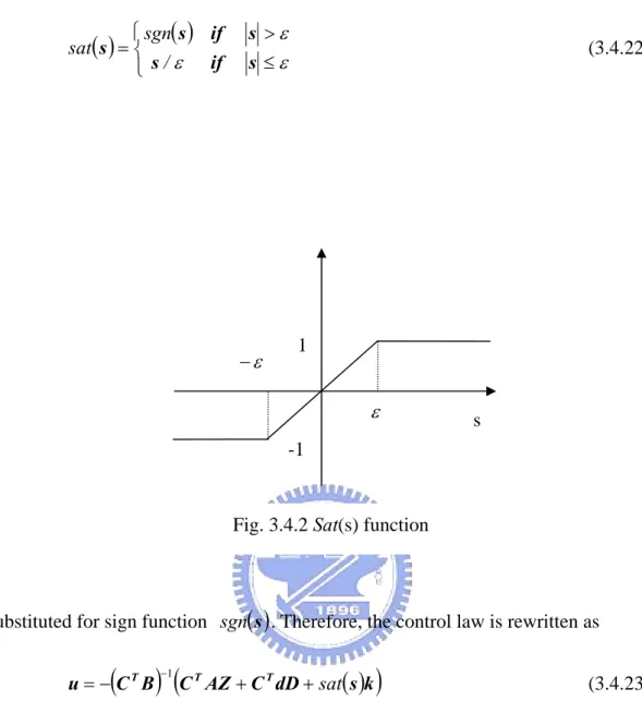
We use the saturation function

( )

s

( )

( )

⎩ ⎨ ⎧ ≤ > = ε ε ε s if s s if s s / sgn sat (3.4.22) 1

substituted for sign function sgn

( )

s . Therefore, the control law is rewritten as

( )

C B

(

C AZ C dD

( )

s k

u₌₋ T −1 T ₊ T _+sat

)

(3.4.23)

Before entering the sliding layer s >ε, the modified control law is the same as the previous one. The control law forces the system trajectory to reach the sliding layer

ε

≤

s in a limit time. When entering the sliding layer, gain of the control law must

be minimized. And, the system can’t maintain zero when there occurs a disturbance. It

means that the control law couldn’t make all states to zero but around zero. The

tradeoff of the decreased precision is that the input chattering effect is slow down and

input gain is decreased. The key point is that the sign function of (3.4.20) is not s

-1 ε

−

ε

realizable in practical because of its infinite switch, and the modified control input

Chapter 4

Simulation Results

4.1 Pole Placement

From Chapter 2, two-element model is chosen as the desired control system [11],

and the flexible model has 10 system poles shown in Fig. 4.1.1. Before system

simulation, the desired system poles should be determined first. In rigid control, the

poles -0.5 and -2 are determined and used in experimental demonstration. Then,

consider about the Sliding mode control, Lyapunov method which has been

introduced in Appendix C is used to design the sliding surface. The system poles of

the control system should be designed in the procedure of applying Lyapunov method.

The desired poles for sliding mode control are shown in Fig. 4.1.2. The dominant

poles of SMC are designed at -0.5 and -2, and the other poles are designed as complex

conjugates lined in 45 degrees to the origin in left half plane. The imaginary part of

original poles (Fig. 4.1.1) and desired poles (Fig. 4.1.2) are of the same value, so that

the sliding surface will let the controller better with low input torque. But, the

shortcoming of the Lyapunov method is that the finally poles of the system may not

achieved which is meant that the system is in sliding surface. However, there is a

significant advantage of the Lyapunov method based on its fundamental algorithm

which is come from energy for the sliding surface design yields the less input torque

required. Not only consider about the limited motor torque in this experiment but also

concern for power consumption, Lyapunov method achieves a good result in input

restricted torque compared with the transformation matrix method. As for PD

controller, it also needs large torque for better transient response [5]. Although the

worse case could be corrected by adding a shaping reference input [13, 4].

-10 -8 -6 -4 -2 0 2 4 6 8 10 -600 -400 -200 0 200 400 600 Pole-Zero Map Real Axis Im ag in ar y A x is

-600 -500 -400 -300 -200 -100 0 -600 -400 -200 0 200 400 600 Im a g in a ry A x is Real Axis Pole Map of SMC

Fig. 4.1.2The desired poles of the sliding mode controller

4.2 Sliding Mode Controller Simulation Results

According to poles placement in section 4.1, the system poles are determined in

sliding mode control. Then, the software Matlab is used to verify the controller. With

the experimental equipment parameters showed in Table 2.4.1, the simulation results

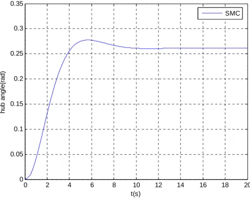
for hub angle regulation are shown in Fig. 4.2.1 to Fig. 4.2.5, and the parameters

01 0. =

0 2 4 6 8 10 12 14 16 18 20 0 0.05 0.1 0.15 0.2 0.25 0.3 0.35 t(s) h ub a ngl e( rad) SMC

Fig. 4.2.1 Hub angle regulation in sliding mode control

0 5 10 15 20 -6 -4 -2 0 2x 10 -4 t(s) v1 (m ) SMC 0 5 10 15 20 -2 -1 0 1x 10 -3 t(s) v2 (m ) SMC 0 5 10 15 20 -15 -10 -5 0 5x 10 -4 t(s) v3 (m ) SMC 0 5 10 15 20 -3 -2 -1 0 1x 10 -3 t(s) v4 (m ) SMC

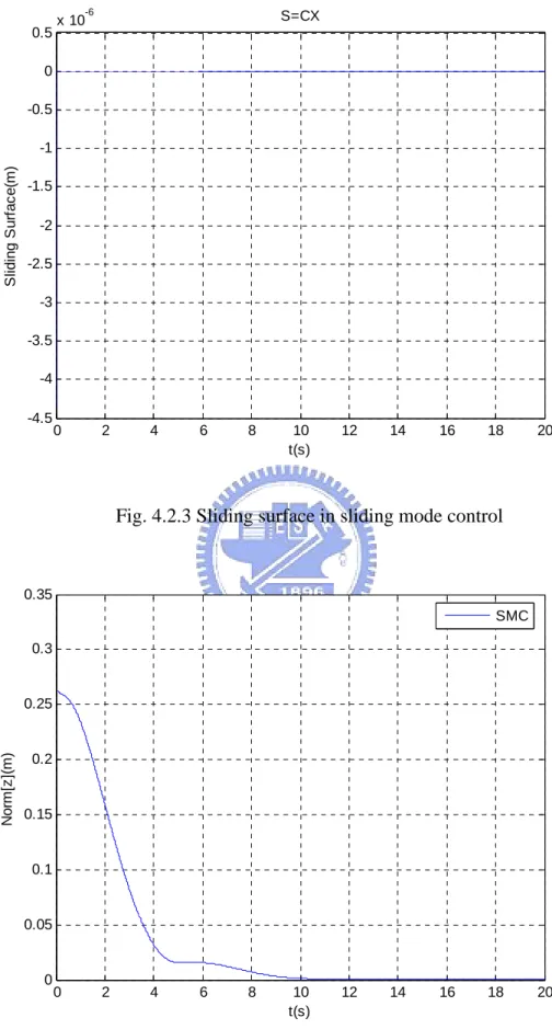
0 2 4 6 8 10 12 14 16 18 20 -4.5 -4 -3.5 -3 -2.5 -2 -1.5 -1 -0.5 0 0.5x 10 -6 t(s) S lid in g S u rf ac e( m ) S=CX

Fig. 4.2.3 Sliding surface in sliding mode control

0 2 4 6 8 10 12 14 16 18 20 0 0.05 0.1 0.15 0.2 0.25 0.3 0.35 t(s) No rm [z ]( m ) SMC

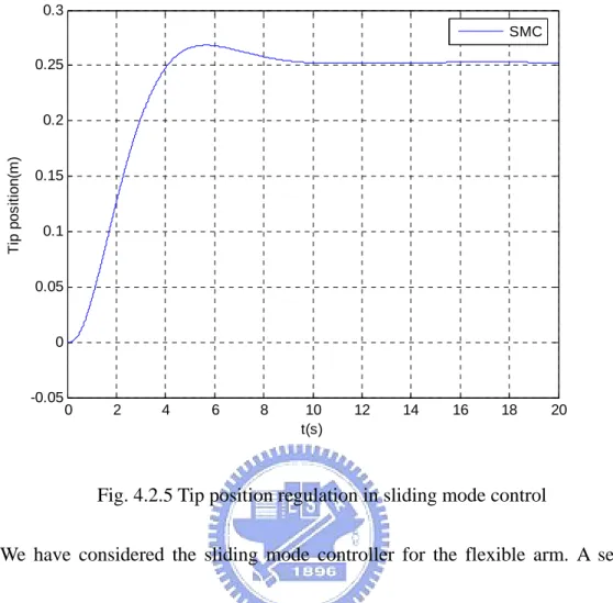
0 2 4 6 8 10 12 14 16 18 20 -0.05 0 0.05 0.1 0.15 0.2 0.25 0.3 t(s) T ip po s it io n (m ) SMC

Fig. 4.2.5 Tip position regulation in sliding mode control

We have considered the sliding mode controller for the flexible arm. A set of

simulation has been carried out. Simulation results confirm that the controller

Chapter 5

Experimental Demonstration

This chapter is about the flexible arm experimental demonstration. The results

will show the sliding mode controller is successful in vibration tolerance and the

developed FEM model of the flexible arm is valid. Compared with the simulation

results, the experimental demonstration makes us convinced of the controller design

in chapter is work. The beginning of this chapter is about experiment setup included

of Matlab xPC target environment, motor setup, and deflection measurement which

are the foundations of experiment.

5.1 Experimental Setup

5.1.1 Matlab xPC Target Environment

This experiment is established in Matlab toolbox-xPC Target. In Fig.5.1.1,

xPC-MC240 I/O card is used to get the angle from the motor and PCI-1716 card is

used to do AD/DA signal convert. The xPC Target is a solution for prototyping,

environment that uses a target PC, separate from a host PC, for running real-time

applications. In this environment the desktop computer as a host PC with Matlab and

Simulink creates a model using Simulink blocks. After creating the model, xPC Target

lets the blocks and a C/C++ compiler to create executable code with its embedded

coder. The executable code is downloaded from the host PC to the target PC running

the xPC Target real-time kernel. After downloading the executive code, the

application can be run by the target PC in real-time. The advantages of xPC Target are

the fast sampling rate to ten thousands Hz in real-time work and it is convenient to

hardware implementation with convenient parameters turning.

Host PC xPC Target PCI-1716 Amp Ckt Strain Guage Phase A B MC240(QEP) Motor Torque xPC Kernel

5.1.2 Motor Setup

The Mitsubishi AC-servo motor HC-KFS 053B and the servo-amplifier

MR-J2S-10A are adapted in the experiment. The specifications of AC-servo motor

HC-KFS 053B is shown below in the table 5.1.2 [20].

Table 5.1.2 Servo Motor Specifications

Maximum torque 0.48[Nm]

Maximum rotation speed 3000[rpm]

Moment of inertia J 0.053[×10−4kgm2]

Position detector 131072p/rev[17-bits]

Maximum current 2.5[A]

Rated current 0.83[A]

Permissible instantaneous rotation speed 5175[r/min] Maximum rotation speed 4500[rpm]

The PCI-1716 card provides a 16-bit resolution AD/DA transformation for strain

feedback and torque driven voltage. The hub angle is detected by the xPC-MC240 I/O

card with a TM S320F240DSP embedded with Quadrature Encoder Pulse (QEP)

circuit. The QEP circuit determines the rotation direction by the input generated by an

optical encoder on a motor shaft, the direction of rotation of the motor can be

determined by detecting which of the two sequences leads. The two sequences are

pulses with variable frequencies and fixed phase shifts of a quarter of a period (90

High-resolution position determination 32768 pulse per revolution is applied in this

experiment.

5.1.3 Deflection Measurement

Several methods have been used to measure the deflections of the arm, such as

Photo-Diodes, Laser Doppler Vibrometers, and Strain gauges. Since strain gauges are

cheap and effective sensors, they are used to measure strains as small as a fewµε in this experiment. A strain gauge is basically a grid of wire or conductor attached to the

arm and changes its conductance as the arm stretches. This change in conductance is

used to find the change in bending moment of the arm. The strainε measured in the

arm is related to the deflection w

( )

x,t as follows [10]:

( )

⎟⎟ ⎟ ⎠ ⎞ ⎜⎜ ⎜ ⎝ ⎛ ⎟ ⎟ ⎠ ⎞ ⎜ ⎜ ⎝ ⎛ ∂ ∂ + ⎟ ⎟ ⎠ ⎞ ⎜ ⎜ ⎝ ⎛ ∂ ∂ + ∂ ∂ = = = = 2 2 2 2 2 2 2 1 2 1 p x p x p x x w x w x t x w , ε (5.1)

where x is the axis parallel to the arm in a stress-free state and p is the distance

between the location strain gauge attached and the root of the arm. However, the

disadvantage of the strain gauges is that they have a maximum strain and might get

damaged subject to higher strains. Only small deflections in the arm are considered.

To precisely detect the distortion of the arm, first determine a certain positions

with explicit deformation and then purposely paste two strain gauges to each of these

positions in the way of face-to-face on both sides. When deformation appears, the

resistance of each strain gauge changes with the variation R∆ . The small variation

R

∆ will be detected by the Wheatstone bridge circuit shown in Fig. 5.1.2.

R R−∆ R+∆R R R 01 V ref V

Fig.5.1.2 Wheatstone Bridge Circuit

The gain of the Wheatstone bridge circuit is

2 2 1 4 2 R R R R V V_{O ref} ∆ ∆ − = (5.2)

The value of is small in (5.2) because of the use of low voltageV to protect

the strain gauges from broken by high temperature due to the high reference voltage.

In this experiment, the reference voltage V is assigned to 5 volt. The voltage

1 O

V _ref

amplifier circuit shown in Fig. 5.1.3 is designed to amplify so that the AD input

will get higher resolution.

1 O V R′ R R′ R1 1 R 2 R 2 R 2 O V 1 O V

Fig.5.1.3 Voltage Amplifier Circuit

The circuit of Fig.5.1.3 which is common used as an industrial voltage amplifier has

high input resistance and good CMRR. The V_O2 could be calculated as

1 1 2 2 2 1 _O O V R R R R V ⎟ × ⎠ ⎞ ⎜ ⎝ ⎛ ₊ ′ = (5.3)

When the resistances R , R′ , , and are chosen in proper values, the proper

gain which limits the A/D input ranged inside

1

R R₂

V

10

± could be achieved. Finally, it is important to design a low pass filter to reduce the high pass noise. The second order

Butterworth filter shown in Fig.5.1.4 is designed and its 3db cutoff frequency

assigned to 250Hz is calculated in (5.4). The frequency response of the filter is shown

( )

₍

₎

₍

₎

1 1 2 1 2 2 2 1 2 1 2 3 + + + = = s R R C s R R C C V V s H O O _(5.4) 3 R R₄ 2 R 3 O V 2 O V 1 C 2 C

Fig.5.1.4 Low Pass Filter Circuit

101 102 103 104 105 -180 -135 -90 -45 0 P h as e ( d e g ) Bode Diagram Frequency (Hz) -100 -80 -60 -40 -20 0 System: ll Frequency (Hz): 250 Magnitude (dB): -3 M a g n itud e ( d B )

Fig.5.1.5 Low Pass Filter Bode Plot

some high impulse noise appears when signal transfers in wires, but it is solved by a

software 80Hz low pass filter in digital before into the digital controller. Until now,

the signals of strain gauges are finally precisely fed back. However, the state feedback

is considered as elements’ position angular variation and angular velocity, so the

mathematical transformation from strain gauges feedback to states needs to derived.

Here, the mathematical transformation in two-element FEM model is considered and

will be shown in the following description. By definitions, the measured amount for a

strain gauge feedback is an external moment applied to a strain gauge position. The

first strain gauges pasted at x₁ to the root can be described as

( )

1 2 1 1 1 2 M x t x w _{= ⋅} ∂ ∂ , _µ (5.5)

The second ones pasted at x₂ to the root can be described as

(

)

2 2 2 2 2 2 M x t x w _{= ⋅} ∂ ∂ , _µ (5.6)

Consider the continuous boundary between two elements, the moment of them must

be the same, so

( )

( )

2 2 2 2 1 1 2 0 x t w x t h w ∂ ∂ = ∂ ∂ , , (5.7)

And, the principle assumption of Euler Bernoulli beam is the zero moment at the arm

tip, so

( )

0 2 2 2 2 = ∂ ∂ x t h w , (5.8)

( )

1 2 1 1 1 2 M x t x w _{= ⋅} ∂ ∂ , _µ

( )

1 2

( )

1 3

( ) ( )

1 1 4

( ) ( )

1 2 1 1 x 0 φ x 0 φ x v t φ x v t µM φ″ ⋅ + ″ ⋅ + ″ ⋅ + ″ ⋅ = (5.9)

(

)

2 2 2 2 2 2 M x t x w _{= ⋅} ∂ ∂ , _µ

( ) ( )

2 1 2

( ) ( )

2 2 3

( ) ( )

2 3 4

( ) ( )

2 4 2 1 x v t φ x v t φ x v t φ x v t µM φ″ ⋅ + ″ ⋅ + ″ ⋅ + ″ ⋅ = (5.10)

( )

( )

2 2 2 2 1 1 2 0 x t w x t h w ∂ ∂ = ∂ ∂ , ,

( ) ( )

h v₁ t ₄

( ) ( )

h v₂ t ₁

( ) ( )

v₁ t ₂

( ) ( )

v₂ t ₃

( ) ( )

v₃ t ₄

( ) ( )

v₄ t 3 0 0 0 0⋅ ″ + ⋅ ″ + ⋅ ″ + ⋅ ″ = ⋅ ″ + ⋅ ″ _{φ φ φ φ φ} φ (5.11)

( )

0 2 2 2 2 = ∂ ∂ x t h w ,

( ) ( )

2 _{1 2}

( ) ( )

2 _{2 3}

( ) ( )

2 _{3 4}

( ) ( )

2 ₄ 0 1 ⋅ = ″ + ⋅ ″ + ⋅ ″ + ⋅ ″ _{h v t φ h v t φ h v t φ h v t} φ (5.12)

Rearrange (5.9) (5.10) (5.11) (5.12) into a matrix form

M v= ⋅ ⋅ µ φ (5.13) where

( )

( )

( )

( )

( )

( )

( )

( )

( )

( )

( )

( )

( )

( )

( )

( )

⎥⎥ ⎥ ⎥ ⎥ ⎦ ⎤ ⎢ ⎢ ⎢ ⎢ ⎢ ⎣ ⎡ ″ ″ ″ ″ ″ ″ ″ ″ ″ ″ ″ − ″ ″ − ″ ″ ″ = h h h h x x x x h h x x 2 2 2 2 0 0 0 0 0 0 4 3 2 1 2 4 2 3 2 2 2 1 4 3 4 2 3 1 1 4 1 3 φ φ φ φ φ φ φ φ φ φ φ φ φ φ φ φ φ (5.14)

( )

( )

( )

( )

⎥⎥ ⎥ ⎥ ⎦ ⎤ ⎢ ⎢ ⎢ ⎢ ⎣ ⎡ = t v t v t v t v v 4 3 2 1 (5.15)

⎥ ⎥ ⎥ ⎥ ⎦ ⎤ ⎢ ⎢ ⎢ ⎢ ⎣ ⎡ = 0 0 2 1 M M M (5.16)

When φ−1 is exist, the flexible arm state variables could be calculated by

M v=_µ⋅_φ−1⋅

(5.17)

Now, we have already described the measurement the strain moments of two elements

of the arm.

5.2 Sliding Mode Controller Experimental Results

Consider the robustness of a variable structure system, there are three kinds of

noises need to be faced [15]. Such as:

A. The disturbance from outside of the plant, such as AC power supply …etc.

B. The uncertainty of the system parameters changes with different environment,

such as changes of temperature.

C. The unmodeled modes are hard to find in the control system.

As a result, Fig. 5.2.1 to Fig. 5.2.3 show the experimental results of the

flexible arm controlled by a rigid controller whose poles designed in -0.5 and -2. This

demonstration shows that these disturbances yield much vibration in rigid controller.

We needs to avoid these noises carefully, or the control goal may be failed, even then

of the control system is an important target in system and controller design. Variable

structure control is well used in practical for the most part of its robustness. The hub

regulation experimental results shown in Fig. 5.2.4 to Fig. 5.2.15 also verify the

advantages of SMC. In these figures, the dominant poles of SMC are designed at -0.5

and -2, and the other poles are designed as complex conjugates lined in 45 degrees to

the origin in left half plane shown in Fig.4.1.1. In Fig.5.2.4 to Fig. 5.2.7, the

parameters are defined as ε =0.01 andσ =5. Then, in Fig.5.2.8 to Fig. 5.2.11, the parameters are defined as ε =0.0067 andσ =6. Finally, in Fig.5.2.12 to Fig. 5.2.15, the parameters are defined as ε =0.005 andσ =8.

0 2 4 6 8 10 12 14 16 18 0 0.05 0.1 0.15 0.2 0.25 0.3 0.35 t(s) hu b angl e( rad) Rigid Control

0 2 4 6 8 10 12 14 16 18 0 0.05 0.1 0.15 0.2 0.25 0.3 0.35 t(s) T ip p o s it ion (m ) Rigid Control

Fig. 5.2.2 Tip position regulation in rigid control

0 5 10 15 20 -5 0 5 10x 10 -4 t(s) v1 (m ) Rigid Control 0 5 10 15 20 -2 0 2 4x 10 -3 t(s) v2 (m ) Rigid Control 0 5 10 15 20 -2 -1 0 1 2x 10 -3 v3 (m ) t(s) Rigid Control 0 5 10 15 20 -2 0 2 4x 10 -3 v4 (m ) t(s) Rigid Control

0 2 4 6 8 10 12 14 16 18 20 0 0.05 0.1 0.15 0.2 0.25 0.3 0.35 t(s) hub a ngl e (r a d ) SMC

Fig. 5.2.4 Hub angle regulation in sliding mode control (ε =0.01 andσ =5)

0 2 4 6 8 10 12 14 16 18 20 0 0.05 0.1 0.15 0.2 0.25 0.3 0.35 t(s) T ip po s it ion( m ) SMC tip position SMC

0 5 10 15 20 0 0.5 1x 10 -3 t(s) v1 (m ) 0 5 10 15 20 -1 0 1 2 3x 10 -3 t(s) v2 (m ) 0 5 10 15 20 -1 0 1 2x 10 -3 v3 (m ) t(s) 0 5 10 15 20 -1 0 1 2 3x 10 -3 v4 (m ) t(s) SMC SMC SMC SMC

Fig. 5.2.6 Four states response in sliding mode control (ε =0.01andσ =5)

0 2 4 6 8 10 12 14 16 18 20 -1.5 -1 -0.5 0 0.5 1 1.5x 10 -4 t(s) S lid ing S u rf ac e( m ) S=CX SMC

0 2 4 6 8 10 12 14 16 18 20 -0.05 0 0.05 0.1 0.15 0.2 0.25 0.3 0.35 t(s) hu b a ngl e( ra d) SMC

Fig. 5.2.8 Hub angle regulation in sliding mode control (ε =0.0067andσ =6)

0 2 4 6 8 10 12 14 16 18 20 -0.05 0 0.05 0.1 0.15 0.2 0.25 0.3 0.35 t(s) T ip pos it ion( m ) SMC tip position SMC

0 5 10 15 20 -5 0 5 10x 10 -4 t(s) v1 (m ) SMC 0 5 10 15 20 -1 0 1 2x 10 -3 t(s) v2 (m ) SMC 0 5 10 15 20 -5 0 5 10 15x 10 -4 v3 (m ) t(s) SMC 0 5 10 15 20 -1 0 1 2x 10 -3 v4 (m ) t(s) SMC

Fig. 5.2.10 Four states response in sliding mode control (ε =0.0067andσ =6)

0 2 4 6 8 10 12 14 16 18 20 -1.5 -1 -0.5 0 0.5 1 1.5x 10 -4 t(s) S lid ing S u rf ac e( m ) S=CX SMC

0 2 4 6 8 10 12 14 16 18 20 0 0.05 0.1 0.15 0.2 0.25 0.3 0.35 t(s) h ub a ngl e( rad) SMC

Fig. 5.2.12 Hub angle regulation in sliding mode control (ε =0.005andσ =8)

0 2 4 6 8 10 12 14 16 18 20 0 0.05 0.1 0.15 0.2 0.25 0.3 0.35 t(s) Tip p o s it io n (m ) SMC tip position SMC

0 5 10 15 20 -2 0 2 4x 10 -3 t(s) v1 (m ) 0 5 10 15 20 -5 0 5 10 15x 10 -3 t(s) v2 (m ) 0 5 10 15 20 -5 0 5 10x 10 -3 v3 (m ) t(s) 0 5 10 15 20 -5 0 5 10 15x 10 -3 v4 (m ) t(s) SMC SMC SMC SMC

Fig. 5.2.14 Four states response in sliding mode control (ε =0.005andσ =8)

0 2 4 6 8 10 12 14 16 18 20 -2 -1.5 -1 -0.5 0 0.5 1 1.5 2x 10 -4 t(s) S lid ing S u rf ac e( m ) S=CX SMC