Modelling, control and simulation of an IC wafer fabrication system: a generalized stochastic coloured timed Petri Net approach

(1)

Modelling, control and simulation of an IC wafer fabrication system: a

generalized stochastic coloured timed Petri Net approach

MING-HUNG LINy and LI-CHEN FU*

This study presents a generalized stochastic coloured timed Petri net(GSCTPN) to model an IC wafer fabrication system. According to the GSCTPN, it models the dynamic behaviours of the IC fabrication system, such as loading, reentrant processing, unloading and machine failure. Furthermore, modular and synthesis techniques are used to construct a large and complex system model. The two major sub-models are the Process-Flow Model and the Transportation Model. The Transportation Model incorporates a simple motion-planning rule and a collision avoidance strategy to solve the variable speed and tra c jam problems of vehicles. This work also describes a simulation based performance analysis and schedule adjustment. To demonstrate the promise of the proposed work, this study makes actual Taiwanese IC wafer fabrication systems the target plant layout for implementation.

1. Introduction

Wafer fabrication is the most expensive phase of semiconductor manufacturing (Sze 1983, Wein et al. 1988, Uzsoy et al. 1992). Signi® cant risk is involved in wafer fabrication because of enormous investment costs. To survive such a competitive and risky environment, the company must not only improve quality and throughput but also satisfy the demands of customers. If product delivery is frequently late, the company loses customer and market goodwill, ultimately in¯ uencing long-term sales opportunities. Additionally, wafer fabrication involves complex processing with operations typically numbering in the hundreds, extending production cycle time. Long production cycle time increases the expense of wafer fabrication because it adversely in¯ uences product yield, and the ability to predict the market trends. Additionally, product life cycles are generally short in the semiconductor industry, and hence, ® nished goods inventories constantly risk obsolescence.

There are many comparative studies and reports (Leachman and Hodges 1996, Robertson and Gargini 1998), which have developed a systematic account of the practices that explain best manufacturing performance in semiconductor production on a world-wide basis. The advent of production 300mm wafer fabs is poised to occur at a time when wafer-processing technology is undergoing rapid changes. The International 300 mm Initiative (I300I) approach for transport of wafers speci® es the front opening uni® ed pod (FOUP) with a capacity of either 13 or 25 wafers (it is a user option as to which is implemented) (Plata 1997, Csatary et al. 1998). The size and weight of the 25 wafer lot/FOUP combination is almost 18 pounds (8.2kg),

International Journal of Production Research ISSN 0020± 7543 print/ISSN 1366± 588X online#2000 Taylor & Francis Ltd http://www.tandf.co.uk/journals

Revision received January 2000

{ Department of Computer Science and Information Engineering, National Taiwan University, Taipei, Taiwan, Republic of China.

(2)

which is beyond the ergonomic limit for repeated manual handling. When the cubic volume of the FOUP is considered, the combined size and weight become important factors for 300mm factory planning.

Automated material handling systems (AMHS) are utilized in almost all 200 mm fabs for transport of wafer lots between the stockers at each process bay (`Interbay transport’). Human operators use transport from the stockers to the process equip-ment (`Intrabay transport’). The Interbay system used most widely is of the overhead track (OHT) type. The Intrabay systems are such as AGVs (automated guided vehicles), RGVs (rail guided vehicles) and so on. It would be expected that the major change in AMHS will occur within the bay. The 300 mm fabs will make use of automated intrabay delivery to each process equipment. This results in mini-mized interference with operators and tool service/maintenance work on the intra-bay material ¯ ow as well as narrow operator aisles. Thus, the material handing system’s basic function is to remove the task of pod handling from the human operators. Reduced mishandling and misprocessing, operator and tool productivity gains, and enhanced material accountability are only a few of the bene® ts (Plata 1997, Csatary et al. 1998, Missale 1998).

The intrabay transport system still requires further development about position-ing accuracy, reliability and operator safety issues. However, even with the use of su cient safety measures at the vehicles, this can cause negative e ects on operator e ciency due to psychological concern (Plata 1997). Service and maintenance work on the equipment front end can block the movement path and seriously a ect wafer lot delivery to equipment ready to process material. The intrabay transport system can be more easily maintained compared to OHT systems since they operate on ¯ oor level. Clearly, a part transportation system is ¯ exible and economical. However, it also produces numerous routing possibilities, complicating the decision problem. Since these IC wafer fabrication systems are dynamic, solutions should maximize the timeliness of their control schedule. It is desirable to respond fast to changes in their internal and external environments.

Machine failures are common in IC fabrication. Machine idleness due to failure hinders throughput and, ultimately, production costs. Therefore, most machines need regular maintenance to ensure high availability (Uzsoy et al. 1992, Johri 1993, Uzsoy et al. 1994, Duenyas et al. 1994, Leachman and Hodges 1996). However, the duration and frequency of periodic maintenance also in¯ uence per-formance. Thus, periodical maintenance is an important consideration in the system model.

Recent works by Uzsoy et al. (1992, 1994) Johri (1993), and Duenyas et al. (1994) highlight the di culties in planning and scheduling wafer fabrication facilities and wafer queues. These works also survey the literature on related topics. E ective shop ¯ oor scheduling can signi® cantly reduce cycle time. The bene® ts of e ective sched-uling include higher machine utilization, shorter cycle time, higher throughput rate, and greater customer satisfaction. This is particularly true in semiconductor manu-facturing, with its rapidly changing markets and complex manufacturing process (Li

et al. 1996, Narahari and Khan 1997, Kim et al. 1998a). Yet, in many wafer

fabrica-tions the product spends more time waiting than actually being processed, so there is great potential for reducing waiting time. Other issues related to wafer fabrication systems have also been considered, such as batch processing systems (Glassey and Weng 1991) and maintenance scheduling as well as sta policy (Mosle et al. 1998). However, since wafer fabrication is a complex discrete event system, schedules

(3)

cannot easily be realized, and thus modelling a complex wafer fabrication manu-facturing system becomes imperative. A good model not only helps schedule employ-ment, but also helps monitor the status of lots and machines e ciently, which helps ® ne tune the scheduling policy.

Petri Net (PN) (Desrochers and Al-Jaar 1994) is important in the modelling. Petri-Net (Murata 1989) is a graphical and mathematical modelling tool applicable to many systems. Petri-Net can be used as a visual-communication aid similarly to ¯ ow charts, block diagrams, and networks. Moreover, tokens simulate the dynamic and concurrent activities of systems. Petri-Net is widely common in traditional com-puter science research, such as communication protocols (Diaz 1982), distributed systems (Ayache et al. 1982), compilers and operating systems (Baer and Ellis 1977). Finally, Petri-Net is highly e ective for modelling (Narahari and Viswanadham 1985, Valavanis 1990), simulating (Valavanis 1990), and scheduling (Bispo et al. 1992) discrete event systems, such as ¯ exible manufacturing systems. It is also useful for designing and implementing controllers for manufacturing (Zhou et al. 1990). In addition, some investigations have concentrated on performance analysis (Ramamoorthy and Ho 1980, Molly 1982, 1985, Hillion and Proth 1989). Nevertheless, the massive complexity of a real-world system tends to engender a large Petri-Net with numerous places and transitions. This kind of large net can be constructed by merging sub-nets. However, performing analysis through the reachability graph or invariance methods is nearly impossible. Hence, many researchers have developed a reduction technique (Lee andd Favrel 1985, Lee et

al. 1987) capable of functioning as a synthesis method if appropriately applied.

Moreover, high-level Petri-Net, such as coloured Petri-Net (Kasturia et al. 1988), or some extended Petri-Net (Valavanis 1990) can be used to overcome graphical complexity.

Using Petri-Net for modelling and performance analysis of IC wafer fabrication system is not new. Previous researches are discussed below. Zhou and Jeng (1998) proposed modelling and analysis of semiconductor manufacturing systems via Petri nets. Zhou reviewed applications of Petri-Net in semiconductor manufacturing auto-mation. It proceeds to discuss the use of modules and a general method for con-structing a system model. Timed Petri-Net are introduced for simulation, performance evaluation, and scheduling purposes. This can be served as a simple tutorial paper. Meanwhile, Srinivasan (1998) modelled the cluster tools in semicon-ductor manufacturing and developed an analytical technique that aims to ® nd the state cycle and state period. Srinivasan has considered only deterministic ® ring delays. Nevertheless, modelling with stochastic ® ring delays is necessary for a prac-tical plant.

Janneck and Naedele (1998) presented a tool called CodeSign and allowed object-oriented design and simulation of high-level timed Petri-Net models. The developed model is compared with a previous spreadsheet model in four con® gura-tions with actual measurements on the machine. Although the results show that a prediction error obtained from CodeSign is smaller than that from the spreadsheet model, the proposed modelling approach can not provide constructions for dynamic model structure. However, it is necessary to adopt abstraction concepts from modern programming languages, such as parametric components. Xiong and Zhou (1998) proposed and evaluated the Petri-Net based hybrid heuristic search strategies and their applications in semiconductor test facility scheduling. Xiong and Zhou described two Petri-Net based heuristic search strategies, called hybrid

(4)

BF-BT and hybrid BT-BF, for scheduling semiconductor test facility. However, in practical plant, it is necessary that a schedule can be ® ne tuned based on simulation to meet rapid changes in system parameters without taking long-run o -line sched-uling again.

Allam and Alla (1998) proposed hybrid Petri-Net as an approximation of discrete Petri-Net to tackle the state explosion problem in analyzing large-scale semiconduc-tor manufacturing systems. However, the hybrid Petri-Net is di cult to analyze. Additionally, Lin and Whung (1998) used the coloured timed Petri-Net (CTPN) to model the furnace in IC wafer fabrication. The dynamic behaviours of a furnace are emulated via the CTPN model. However, the CTPN model is not hierarchical and not easy enough to use. Jeng et al. (1998) reported a project of applying Petri-Net to detailed modelling, qualitative analysis, and performance evaluation of the etching area in an IC wafer fabrication system. This model deals with only one type of wafer. It is necessary to consider multiple types of wafers. Furthermore, the proposed model must extend the modular modelling approach and formally de® ne the class of systems.

This work di ers from others in many details. First, it proposes a systematic means of constructing a generalized stochastic coloured timed Petri-Net (GSCTPN) model for modelling an IC wafer fabrication system. However, designing a Petri-Net model for an IC wafer fabrication system is extremely tedious and has debugging di culties. It is necessary to adopt abstraction concepts from modern programming languages, such as parametric components. This systematic modelling method can be implemented as an automatic Petri-Net generator (APNG). Using such generators, building a Petri-Net model of a FMS is no longer di cult and time consuming. The user merely needs to input the system information of a practical wafer fabrication system, such as the number of automated guided vehicles (AGVs), the number of machines and their geometric relationships, and the process ¯ ows of parts requiring processing. Furthermore, the proposed GSCTPN model considers multiple types of wafers. Second, the proposed GSCTPN model extends the modular modelling approach and formally de® nes the class of systems that can be dealt with using the approach. For multiple-load and variable-speed automated guided vehicle (AGV) systems, the GSCTPN model has a control rule already embedded into it to prevent vehicle collision problems. The transporting system again aims to intro-duce a control method into the Petri-Net model to ensure a jam-free condition among carriers. Third, this study describes a simulation based performance analysis and schedule adjustment. A schedule can be ® ne tuned based on simulation to meet rapid changes in system parameters without taking long run o -line scheduling again. The resulting net model is checked for important qualitative properties in IC fabrication systems. Simulation is used to obtain performance measures. The validated model can be used to answer many `what-if ’ questions, such as predicting the throughput. To demonstrate the promise of the proposed work, a real-word IC wafer fabrication system located in Taiwan is used as a target plant layout for implementation.

The rest of this paper is organized as follows. Section 2 describes an IC wafer fabrication system. Section 3 introduces a GSCTPN systematic system modelling method. Section 4 presents simple control policies for AGV, lot release and lot scheduling. Section 5 describes simulation based performance analysis and schedule adjustment. Conclusions are ® nally made in Section 6.

(5)

2. System description

2.1. IC wafer fabrication process

IC wafer fabrication is a multi-stage process with reentrant ¯ ows. A typical wafer undergoes hundreds of processing steps using di erent machines over several weeks. These steps include oxidization, photo resistor coating, developing, etching, ion doping, chemical deposition, and di usion. Generally, the machines in an IC wafer fabrication system are grouped into four functional sections: the

photolitho-graphy area, the di usion area, the etching area, and the thin ® lm area.

The wafer processing unit in IC wafer fabrication is called a lot. When lots arrive at the IC factory, they are processed in the above mentioned four areas. The photo area arranges patterns of photo resistors on wafer. After processing in the photo area, wafers usually go to the etching area, where the part of wafers not covered by photo resistors is etched. The di usion area and the thin ® lm area deposit some material or implant ions on the wafers.

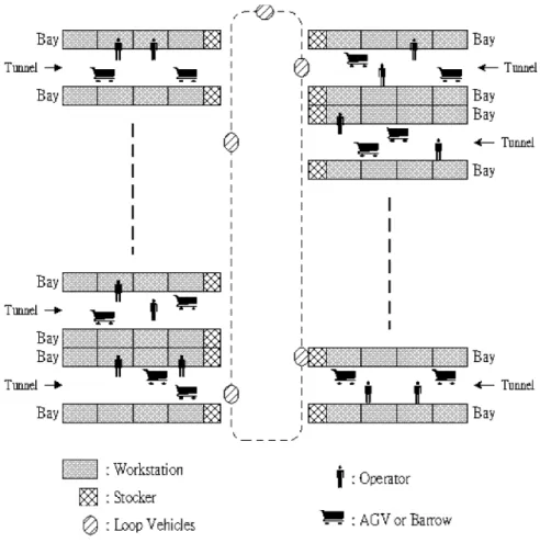
Figure 1 indicates that an IC plant is a base of tunnels. Tunnels in the same area are located in close proximity to each other to reduce wafer transportation time. Machines are sited beside the tunnels, and grouped into a bay. Generally, automated material handling system in IC wafer fabrication comprises two subsystems: Interbay

(6)

system and Intrabay system. Multiple automated guided vehicles (AGVs) are used

for wafer transportation. Each AGV carries multiple loads, and has variable speed. AGVs are allowed to accelerate in movement. In the Interbay system, AGV are called loop vehicles which can move to any stop unidirectionally. Each stop in Interbay serves a transit station transporting lots between di erent Intrabays. The transit stations are denoted as Interbay stations. However, the Intrabay system is composed of several independent tracks. Tracks in di erent area are not overlap-ping. Meanwhile, tracks in the Intrabay system are more comprehensive. When an AGV wants to move between stops within the same area, it has many routing choices. Meanwhile, three phases must be completed if the system wants to transport lots between stops located in di erent bays. First, an AGV transports lots to the Interbay station. Next, a loop vehicle takes the lots to the Interbay station of the destination bay. Finally, an AGV transports the lots to the destination stop. The performance of the AGV greatly a ects the overall performance. Thus, the AGV dispatching, AGV routing and tra c jam problems of vehicles must be considered to maximize performance.

2.2. Hierarchical view of ¯ exible wafer fabrication system

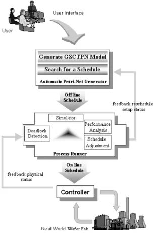
Figure 2 represents a hierarchical view of a ¯ exible wafer fabrication system. This work develops a Petri-Net model for a wafer fabrication system and gives a

(7)

tion-based performance analysis and schedule adjustment. The automatic Petri-Net generator (APNG) developed herein has a graphic user interface that permits users to input the speci® cations of a wafer fabrication system, based on which, the opera-tor can create a GSCTPN model of the wafer fabrication system. Considering the Petri-Net model features, a feasible ® ring sequence can be found by following a path from the initial marking to the ® nal marking. However, each marking of a Petri-Net represents a system state. Thus, the system time is continuously monitored in a timed place Petri-Net. Consequently, the transitions of ® ring sequence can represent part processing routes, shared resource use, and the timing of events in these events.

In the Petri-Net model, an o -line schedule for the system can be obtained using the queuing theory approach (Rogers and White 1991), mathematical programming (France 1982, Sarin et al. 1988, Agnetis et al. 1990, Hoitomt 1990, Luh 1990, Sawik 1990, Rogers and White 1991) heuristic algorithms (France 1982, Anderson and Nyirenda 1990, Mahmoodi et al.1990, Rao and Wang 1991), or the arti® cial intelli-gence approach (Chen et al. 1987, Shaw 1988, Lee and DiCesare 1992). In fact, this o -line schedule is not yet ready for running. Therefore, it is inputted to a so called

process runner to eventually produce an on-line schedule which will drive the

con-troller to control the real world wafer fabrication system. Therefore, the entire structure Figure 2 depicts constitutes a dynamic scheduler. Notably, the process

runner contains three major components, (1) a schedule adjuster, used to adjust

the o -line schedule to cope with events such as the delay of an AGV arrival or a machine break down; (2) simulator, used to simulate the environment of the real world wafer fabrication system and provide the basis for issuing a search; and (3) deadlock detection mechanism, which detects and avoids potential deadlocks. Furthermore, the controller not only controls each real physical object but also adjusts the physical status to the process runner so the simulator can use feedback data to update the simulation database.

Most scheduling, planning, or layout problems depend on resolving the optimi-zation methods algorithm. However, the criteria represented in analytic form are NP-hard problems. Simulation with discrete events has shown e cient in analyzing production systems. Several stochastic methods exist for avoiding local optimum caused by simulation. The joint use of simulation models and optimization methods has been widely studied (Dolgui and O® tserov 1997). This investigation describes a schedule adjustment method that uses data from the previous optimization method to ® nd a new starting point that approach the optimum. When the environmental parameters slightly change, the optimal schedule can be ® ne tuned based on simula-tion to produce a new on-line schedule, and to keep pace with rapidly changing system parameters without requiring lengthy o -line scheduling.

A systematic modelling method requires several sub-models to simulate the job shop problem in a wafer fabrication system. These sub-models can model the material handling systems and part processing under precedence constraints. Before the modelling, a model relation graph is depicted in Figure 3. The model proposed here is a general model, which does not focus on special cases. Restated, once the equipment information is provided, the model generator automatically generates the wafer-processing model. This model can support numerous process ¯ ows of di erent products by changing the token colour, provided these process ¯ ows are performed in the fab using the proposed generalized stochastic coloured timed Petri-Net (GSCTPN) model. The following section describes the details of the proposed Process Flow Model and Transportation Model.

(8)

3. Generalized stochastic coloured timed Petri-Net modelling 3.1. Preliminaries

The proposed generalized stochastic coloured timed Petri-Net (GSCTPN) extends the framework of the original PN with colour, time and modular attributes. The GSCTPN also permits the use of inhibitor arcs and random switches. Inhibitor arcs prevent transitions from ® ring when certain conditions are true. Meanwhile, the random switch resolves con¯ icts between two or more immediate transitions. The GSCTPN contains immediate transition and transitions with exponentially distrib-uted ® ring times. Hereon, for simplicity, the latter are referred to as exponential transitions. Markings within which at least one immediate transition is enabled are called vanishing markings. Meanwhile, markings within which only exponential transitions are enabled are called tangible markings. With a tangible marking, any enabled transition can ® re next. The actual transition that ® res depends on the ® ring rates of the enabled exponential transitions. For a vanishing marking, only the enabled immediate transitions are allowed to ® re.

The GSCTPN model in this work contains two major sub-models. One is called the Transportation Model, while the other is called the Process Flow Model. Both models are ¯ exible. The Transportation Model attempts to model the lot transporta-tion, AGV motransporta-tion, and AGV travelling. Meanwhile, the Process Flow Model attempts to model lot routing, reentrant processing, machine failure, and periodic maintenance. The two sub-models, of course, interconnect to respond to the triggers from each other.

The GSCTPN model presented herein classi® es the places and transitions into the ® ve categories listed below:

Resource Places model production resources like transportation carriers, machines, and the control right of AGV stops in the transportation system. If a resource place is marked, the resources corresponding to marked resource places are free and available.

(9)

Intermediate places model the process ¯ ow of a lot or the movement of an AGV. Marked intermediate places, indicate that the last operation of a lot or the last movement of an AGV has been completed and that the intermediate place is ready for the next action.

Communication places represent the signals or conditions that are sent to or received from the other sub-models to signal upcoming events. Communication places are also used to link di erent modules. Based on communication places, a hierarch-ical and modular model of wafer fabrication can be developed.

Operation transitions represent that a speci® c operation is in progress. Of course, each transition is associated with an exponentially distributed ® ring time. The association is according to the colour set of input places.

Intermediate transitions model the satisfaction of conditions. For con¯ icting enabled immediate transitions, only one transition is allowed to ® re at a time according to a prede® ned probability distribution. In this model, a constant or a marking-dependent function that depends on the processing steps of a lot is su cient to specify the ® ring of the transitions. To model the technological precedence con-straints for processing lots, the planned transitions according to the prede® ned processing ¯ ow are assigned high probability.

3.2. Modelling for process ¯ ow

The process ¯ ow model can be separated into two micro-models, each with di erent characteristics. One is the process routing module and the other is process elementary module. The following describes each micro-model in detail.

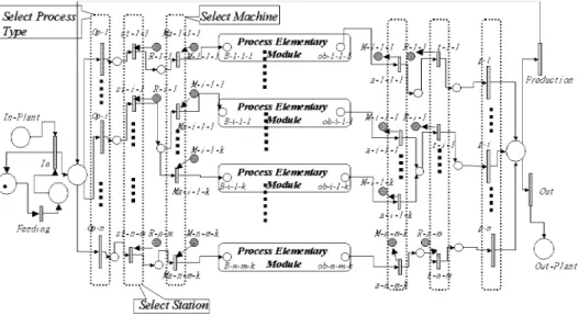
3.2.1. Process routing module

The process routing module models the logical process ¯ ow of the manufacturing systems. The basic concept of this module is as follows. First, the machines in the fab are divided into n workstations (machine groups or processing unit family), each containing one or more identical machines (or processing units). Initially, a token (lot) with the colour xy000 enters the model, where xy is the route ID, and 000 is current operation step. Lots then check-in and their colour is changed to xy001, in preparation for the ® rst operation. Each operation has an associated workstation, thus resulting in much travel to the proper workstation in the fab and operations are performed according to the prede® ned process ¯ ow. After the lot completes the current operation, its colour number is increased by one, and it is ready to undergo the next operation. Systematically, after the lot completes all the operations, it reaches the ® nish.

A lot is released into the IC plant according to certain rules, which can be called

lot release rules. Furthermore, before a lot is fed into workstations for operation, it

must make a sequence of choices and acquire resource usage rights in terms of a token. A lot will undergo service in three phases. First, an operation type is selected for the lot according to prede® ned processing ¯ ow. Second, check that it is the lot that does the choosing an available workstation. Third, check that it is the lot that does the selecting of an available machine. After ® nishing operations, the lot releases each resource. The notations of transitions and places used in Figure 4 are explained as follows:

(10)

R-i-j The place R-i-j is a resource place. It can be conceived of as the control right

of using the j-th workstation of the i-th type of operation.

M-i-j-l The place M-i-j-l is a resource place. It represents the control right of the

l-th machine of l-the j-l-th workstation for l-the i-l-th type of operation. k is total number of machines at the j-th workstation.

In-plant The place in-plant is an intermediate place. When a lot is released to the

fab, a token with the colour (i.e., xy000) is placed here.

Out-plant The place out-plant is an intermediate place. A token at out-plant

repre-sents that the corresponding lot has completed all the operations and is ready to move.

B-i-j-l The place B-i-j-l is a communication place. A token at B-i-j-l indicates the lot

is ready for processing by the machine Mac-i-j-l.

ob-i-j-l The place ob-i-j-l is a communication place. A token at ob-i-j-l indicates the

lot processing has ® nished.

Feeding It is an operation transition. When Feeding is ® red, the colour number of

the token that ® red the Feeding increases by one. This event signi® es that a lot is released into the fab and prepared for the ® rst operation.

In It is an intermediate transition.

Out When the transition Out is ® red, the lot has completed all operations and

entered Out-Plant.

Production The transition Productionis an intermediate transition. When Production is ® red, the colour number of the token that ® red the Production

increases by one. This increase represents that the corresponding lot has ® nished the current operation and is ready for the next operation.

Op-i The transition Op-i is an intermediate transition. It indicates that lots select an

operation type according to prede® ned processing ¯ ows. Figure 4. Process routing module.

(11)

st-i-j similarly, the transition st-i-j is also an intermediate transition. It indicates

that lots choose one workstation from among those available according to a prede® ned processing ¯ ow.

Ma-i-j-l The transition Ma-i-j-l is also an intermediate transition. It represents that

a lot has selected one of the machines available at the j-th workstation according to prede® ned processing ¯ ow or random choice.

Op-i Finally, the transition Op-i is another intermediate transition. It has a colour

set that denotes the coloured tokens that can be ® red through this transition. 3.2.2. Process elementary module

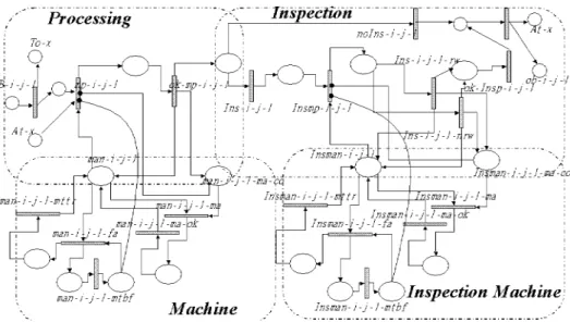
The process elementary module comprises four subnets as Figure 5 displays, each with di erent characteristics. The four subnets are, the processing subnet, inspection subnet, machine subnet, and inspection machine subnet. However, the inspection subnet and inspection machine subnet have to be added if wafers require inspection. The following are detailed descriptions of each of these subnets.

3.2.3. Processing subnet

According to Figure 5, the essential idea of modelling processing subnet is that, before a lot can monopolize any resources, it must acquire its control right via a token.

man-i-j-l The place man-i-j-l is a resource place. It represents that if a lot wants to

move to the machine Mac-i-j-l located at the stop x, it must acquire the token of the resource place man-i-j-l.

T o-x The place To-x is a communication place. If the current location of the wafer

di ers from that of machine Mac-i-j-l, a signal must be sent to the communica-tion place To-x. This signal calls an AGV to come to the place where the wafer resides.

(12)

At-x The place At-x is a communication place. When the AGV arrives, it loads the

wafer. The AGV then starts to move to the destination. Finally, when the AGV reaches the destination, starts the unloading and releases the loading space of the AGV, a token is moved into the communication place At-x.

mp-i-j-l The transition mp-i-j-l is an operation transition. The mp-i-j-l is associated

with exponentially distributed ® ring times according to the colour set of input places. As mentioned before, the colour set represents the current step of the process ¯ ow, implying that operating time can depend on the current step number of a lot and lot type.

3.2.5. Inspection subnet

According to Figure 5, wafers may or may not be inspected and reprocessed for some operations. For example, if photo resistors are not completely removed in etching, the step is repeated.

noIns-i-j-l The transition noIns-i-j-l is an intermediate transition. If wafer

inspec-tion is not required, the intermediate transiinspec-tion noIns-i-j-l is ® red.

Insmp-i-j-l The transition Insmp-i-j-l is an operation transition. The operation

transition Insmp-i-j-l represents the inspection operation. The inspection time also depends on the current step number of the lot and lot type.

Ins-i-j-l-rw The transition Ins-i-j-l-rw is an intermediate transition. If a test wafer of

a lot fails an inspection, the intermediate transition Ins-i-j-l-rw will be ® red.

Ins-i-j-l-nrw The transition Ins-i-j-l-nrw is an intermediate transition. If the

inter-mediate transition Ins-i-j-l-rw ® res, the interinter-mediate transition Ins-i-j-l-nrw also ® res. In practice, only one is allowed to ® re at a time according to the fabrication statistics. Finally, tokens are moved into both communication places At-x and

ob-i-j-l. This process signals the completion of the current processing step.

3.2.5. Machine subnet and inspection machine subnet

According to Figure 5, machine failure is common in IC fabrication.

man-i-j-l-mtbf The transition man-i-j-l-mtbf is an operation transition. The

opera-tion transiopera-tion man-i-j-l-mtbf must be ® red periodically, according to the fabrica-tion statistics. This phenomena is called mean time between failure (MTBF).

man-i-j-l-fa The transition man-i-j-l-fa is an intermediate transition. If transition man-i-j-l-mtbf is ® red, intermediate transition man-i-j-l-fa is enabled and will be

® red immediately. When man-i-j-l-fa is ® red, a token leaves the resource place

man-i-j-l.

man-i-j-l-mttr Transition man-i-j-l-mttr is an operation transition. The repair time

is called mean time to repair (MTTR). After the operation transition

man-i-j-l-mttr, the machine repair is complete and the token returns to place man-i-j-l. i-j-l-ma-co The place i-j-l-ma-co is a communication place. Machines need regular

maintenance. Initially, communication place )i-j-l-ma-co is empty. The output arc weight for place i-j-l-ma-co is man-i-j-l-ma-th.

man-i-j-l-ma The transition man-i-j-l-ma is an operation transition. Once transition mp-i-j-l has ® red man-i-j-l-ma-th times, the operation transition man-i-j-l-ma

(13)

man-i-j-l-ma-ok The transition man-i-j-l-ma-ok is an intermediate transition. Once

the associated time of j-l-ma has passed, the intermediate transition

man-i-j-l-ma-ok ® res, and the token returns to place it man-i-j-l. Transitions and places

in the Inspection Machine subnet, resemble those in the machine subnet. 3.3. Modelling for transportation system

The transportation model can be broken into several micro-models, each with di erent characteristics. They are, the AGV-calling module, AGV-calling dispatch-ing module, AGV-visitdispatch-ing planndispatch-ing module, AGV idle module, AGV routdispatch-ing module, AGV motion planning module, AGV motion control module, and AGV movement module. Each micro model is described in detail as follows.

3.3.1. AGV -calling dispatching module

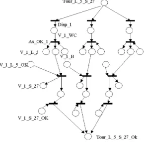
T our_L _x_S_ y: The place Tour_L _x_S_ y is a communication place. A token in

this place implies that wafer will have a tour loaded from the stop x and stored at the stop y.

T our_L _x_S_ y_ok : The place Tour_L _x_S_ y_ok is a communication place. A

token in the communication place T our_L _x_S_ y_ok indicates that the trans-porting tour from stop successfully.

According to Figure 6, a lot is currently located at stop 5 and the next serving workstation is located at stop 19. The place T our_L _5_S_27 is a communication place. Before the next operation, the communication place T o-19 is marked to signal AGV and invokes an AGV to come to the location of the wafer. Stop 19 is located in a di erent bay, and it must be completed with the following steps. First, the com-munication place T our_L _5_S_27 is marked. This marking means that wafer will have a tour loading from stop 5 and storing at stop 27. When the AGV arrives, it loads the wafer. The AGV then moves to the interbay station 27. The place

T our_L _5_S_27_ok is a communication place. A token in communication place

(14)

T our_L _5_S_27_ok signi® es that the transporting tour from stop 5 to stop 27 has

successfully ® nished. Next, the loop vehicle takes lots from interbay station 27 to 32. Finally, an AGV at the destination-bay transports lots from interbay station 32 to the destination stop 19. When the AGV arrives at stop 19, it proceeds to store the wafer. A token at communication place T our_L _32_S_19_ok reveals that the trans-porting tour from 32 to 19 is completed. Finally, a token enters communication place

At-19. This event indicates that the next operation will start.

3.3.2. AGV ± calling dispatching module

Two issues in the AGV-calling dispatching module are AGV-calling dispatching and precedence constraints for transporting.

V _x_W C: The place V _x_W C is an intermediate place. When a token enters the

intermediate place V _x_W C it means that a lot is waiting for AGV x to transport it.

Disp_x: The transition Disp_x is also an intermediate transition. If AGV x is

selected, the intermediate transition Disp_x ® res.

V _x_B : Meanwhile, place V _x_B is a resource place. If the bu er of selected AGV x has free space, the resource place V _x_B is marked.

As_OK_x: The transition As_OK_x is an intermediate transition.

V _x_L _ y: Meanwhile, the place V _x_L _ y is a communication place. That a token

in this place represents that a signal is generated to invoke an AGV x to come to the place y of the wafer.

V _x_L _ y_OK: The place V _x_L _ y_OK is another communication place. If the

communication place V _x_L _ y_OK is marked, it indicates that AGV x has arrived at the stop y and ® nished loading the wafer.

V _x_S_ y: The place V _x_S_ y is a communication place. That a token in this place

represents that a signal is generated to invoke an AGV x to come to the stop y for storage at the location of the wafer.

V _x_S_ y_OK: The place V _x_S_ y_OK is also a communication place. If the

communication place V _x_S_ y_OK is marked, it indicates that AGV x has arrived at stop y and has ® nished storing the wafer.

Figure 7 illustrates, that, for example, the presence of a token at the communica-tion place T our_L _5_S_27, signals that a lot transporting is to be served. The trans-portation is completed in two stages. First, an AGV is chosen according to the dispatching policy. A good dispatching policy can increase AGV utilization. Initially, three AGVs are assumed to be in the intrabay 1. If AGV 1 is selected, the intermediate transition Disp_1 is ® red. When a token enters the intermediate place V _1_W C, it means that a lot is waiting for AGV 1 to transport it. If the bu er of selected AGV contains free space, the resource place V _1_B is marked, and ® ring of the intermediate transition As_OK_1 is enabled.

Next, precedence constraints for transporting lots are considered. The time that the AGV takes to load one lot must happen before storing it. When the intermediate transition As_OK_1 ® res, the communication place V _1_L _5 is marked. The mark-ing represents that a signal is generated to invoke an AGV 1 to come to location of the wafer. If the communication place V _1_L _5_OK is marked, it indicates that AGV 1 has arrived and ® nished loading the wafer. When the communication

(15)

place V _1_S_27 is marked, it represents that the system invokes an AGV 1 trans-porting wafer from stop 5 to stop 27 for storage. Meanwhile, a situation in which the communication place V _1_S_27_OK is marked implies that AGV 1 has arrived at stop 27 and has ® nished storing the wafer. Finally, when the lot tour is ® nished successfully, the communication place Tour_L _5_S_27 is marked.

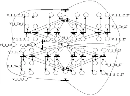
3.3.3. AGV ± visiting planning module

Each multiple-load AGV may have to visit several stop points for loading or storing wafers. Thus, good route planning is needed to solve vehicle tra c jam problems.

V _x_T o_ y: The place V _x_T o_ y is a communication place, and a token there

represents that AGV x must visit stop y.

V _x_L _C_ y: The place V _x_L _C_ y is also a communication place, and a token

there indicates that the goal of AGV x is to load a lot at stop y.

V _x_S_C_ y: Also, the place V _x_S_C_ y is a communication place, and a token at

place V _x_S_C_ y indicates that the goal of AGV x is to store a lot at stop y.

V i_x_OK: Meanwhile, the place V i_x_OK is another communication place, and

when it has a token, it indicates that the current visit is ® nished and the AGV proceeds to the next visit.

V _x_Idle : Finally, the place V _x_Idle is also a communication place. If no visiting

queues exist, the communication place V _x_Idle will be marked, indicating that AGV x is idle.

For example, there are eight stops(2,3,4,5,6,7,26,27) in intrabay 1. Figure 8 illus-trates that if the communication place V _1_L _5 is marked, AGV 1 must go to stop 5 to load a lot. After this, the communication places V _1_T o_5 and V _1_L _C_5 are both marked. If the communication place V _1_S_27 is marked, it means that AGV 1 must arrive at stop 27 for storing.

(16)

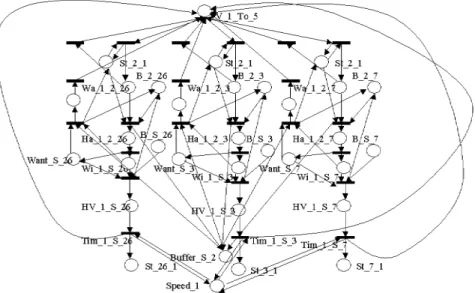
3.3.4. AGV routing module

The AGV routing module corresponds to the decision-making model for AGV routing. Each time an AGV wants to change stops, it must ® rst decide its route. Once the routing decision is be determined the AGV can move along that route. Therefore, for each stop, a corresponding Petri-Net model is necessary to take care of the routing decision. Generally, stops and tracks are assumed to have a capacity of more than one. The basic concept of this model is as follows. When an AGV moves from its current stop to the adjacent stop, two steps are necessary. Firstly, the AGV needs to receive the `right’ to move on the relevant track. If the `right’ is not granted, the next stop on the route may be reselected. If this condition is satis® ed, the AGV can begin travelling on that track.

W a_x_ y_z: The place W a_x_ y_z is an intermediate place. If AGV x at current

stop y selects adjacent stop z as its route, the intermediate place W a_x_ y_z is marked.

B_ y_z: The place B_ y_z is a resource place. If the resource place B_ y_z has

tokens, it represents that the `right’ is ready.

Ha_x_ y_z: The place Ha_x_ y_z is an intermediate place. W i_x_S_z : The place W i_x_S_z is also an intermediate place.

W ant_S_z : Meanwhile, the place W ant_S_z is a communication place,

represent-ing that AGV x is travellrepresent-ing to the stop z. Simultaneously, the control right of the stop y will be released to allow another AGV to use it as a destination or pass-by stop. A token in the communication place W ant_S_z also represents that AGV x broadcasts a `right wanted’ message to each of the idle AGVs.

B_S_z : The place B_S_z is a resource place. The AGV must acquire the control

right of the selected stop to ensure that the bu er of the stop has free space. If the Figure 8. AGV-Visiting planning module.

(17)

resource place B_S_z contains tokens, it represents the bu er has free space or some idle AGVs had left from stop z.

HV _x_S_z : The place HV _x_S_z is an intermediate place.

T im_x_S_z : The transition T im_x_S_z is an operation transition. If the

intermedi-ate place HV_x_S_z is marked, the operation transition Tim_x_S_z is enabled and AGV x can enter the adjacent stop z. Therefore, if no tokens remain in the resource place B_S_z, a back moving will occur. The ownership right of the track will be released to allow another AGV to use it, and the resource place B_ y_z to contain a token again.

Speed_x : The place Speed_x is a communication place. A token in colour set of

communication place Speed_x represents the speed of AGV x at that time. The presence of the token implies that variable-speed AGV may consume a di erent amount of time for each journey to the adjacent stop.

St_z_x : The place St_z_x is an intermediate place that indicates that the current

location of AGV x is the stop z. However, the stop z is not the goal stop w, a token is returned to the communication place VxTow.

For example, Figure 9 reveals the AGV routing module which guides an AGV to move from the current stop 2 to stop 5. If AGV 1 selects adjacent stop 7 as its route, the intermediate place W a_1_2_7 is marked if the resource place B_2_7 contains tokens. Meanwhile, when the intermediate places Ha_1_2_7 are marked, tokens immediately enter both of the intermediate places W i_1_S_7 and the communication place W ant_S_7. This behaviour represents that AGV 1 is travelling to stop 7. If the resource place B_S_7 contains tokens, it represents the bu er has free space or some idle AGVs had left stop. In this situation, the intermediate place HV _1_S_7 is marked. The operation transition T im_1_S_7 is enabled and AGV 1 can enter the adjacent stop 7. The operation transition Tim_1_S_7 is associated with a ® ring time

(18)

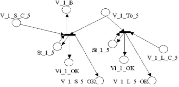
according to the colour set of input place Speed_1. After the time associated with operation transition T im_1_S_7 has passed, the intermediate place St_7_1 is marked. When AGV 1 arrives at stop 5 as Figure 10, one of two transitions ® re according to the status of the communication place V _1_L _C_5 and the communication place

V _1_S_C_5. A token enters the communication place V i_1_O K, signals the

AGV-visiting planning module that current AGV-visiting is completed. After this, the AGV proceeds to the next visiting. Either of the communication places V _1_S_5_O K and V _1_L _5_OK may be marked. The marking represents that a signal has been sent to the AGV-calling dispatching module to con® rm that loading or storing at stop 5 is completed.

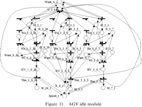
3.3.5. AGV idle module

Notably, until now the AGV routing module has already embedded a control rule into it to prevent vehicle collision problems. In an IC fabrication system, the transporting system may have more than one carrier to transport materials among di erent workstations. However, collision problems no longer exist and, hence, tra c jam problems due to multiple carriers must be solved. In the AGV routing module, the AGV can select the available adjacent stop to achieve partially jam-free conditions among carriers.

The AGV idle module aims to introduce a control method into the Petri-Net model to guarantee jam-free conditions. The method provided is called recursively

leaving strategy, whose basic idea is described below. When a missioned AGV wants

to proceed to a stop, it sends a message to the AGVs that occupy the stop. An idle AGV is selected and it leaves that stop.

places and transitions: The notations of places and transitions are the same with

those in the AGV routing module.

For example as Figure 11 indicates, if the communication place V _1_Idle is marked, it represents that AGV 1 is idle. If AGV 1 is currently at stop 2, a token in communication place W ant_S_2 means that a missioned AGV wants to move to stop 2 but that stop 2 is occupied. Only one idle AGV will be selected to leave stop 2. In this example, the AGV 1 is selected. After a message `Want_S_2’ is sent to the idle AGV 1, it starts to move to the next adjacent stop and leaves its previous location unoccupied. After this, the communication place B_S_2 is marked. Then, if all sub-sequent adjacent stops are occupied, another idle AGV on the adjacent stops will leave. This recursive processing continues until the jam-free conditions are satis® ed. However, the layout geometry and the number of AGVs limit the e ectiveness of this recursive departure strategy. When the number of AGVs increases, the frequency of

(19)

issuing the `Want’ message is quite high. This implies that the system performance will deteriorate.

3.3.6. AGV movement module

Multiple automated guided vehicles (AGVs) are used for wafer transportation. Each AGV carries a multiple-load, and can move at variable speeds. The AGV movement module attempts to model the characteristics of AGV movement. The AGV movement module models the complete behaviour of AGVs which are in transit except for the actions of loading and unloading.

V _x_A : The place V _x_A is a communication place which represents that a `start

accelerating’ command is generated for AGV x.

V _x_ST : The place V _x_ST is an intermediate place which represents that the

status of movement of AGV x has reached the stop stage.

V _x_AC: The place V _x_AC is an intermediate place, indicating that the status of

movement of AGV x has reached the accelerating stage. If AGV x is at the `stop’ stage and the communication place V _x_A is marked, AGV x will proceed to the `accelerating’ stage, and mark the intermediate place V _x_AC.

V _x_CV : The place V _x_CV is an intermediate place which indicates that the

status of movement of AGV x is at the constant-speed stage. However, if both the intermediate place V _x_CV and the communication place V _x_A are marked, it indicates that there is a `start accelerating’ command. Then, the AGV x will enter the `accelerating’ stage and the intermediate place V _x_AC will be marked.

V _x_DA: The place V _x_D A is a communication place, which signi® es that a `start

decelerating’ command is generated for AGV x. Figure 11. AGV idle module.

(20)

V _x_DAC: The place V _x_DAC is an intermediate place, representing that the

status of movement of AGV x is at the decelerating stage. If tokens are both at the intermediate place V _x_CV and the communication place V _x_DA, it represents that a `start decelerating’ command is to be generated. The intermedi-ate place V _x_D AC will be marked.

V _x_NDA: The place V _x_NDA is a communication place, representing that a

`stop decelerating’ command is generated for AGV x.

For example, as Figure 12 indicates, the status of AGV 1’s movement can be classi® ed into four stages, namely, V_1_ST, V_1_AC, V_1_CV and V_1_DAC. When the AGV moves into the `constant-speed’ stage when the speed is not equal to zero. Otherwise, AGV moves into the `stop’ stage and the intermediate places

V _1_ST is marked.

3.3.7. AGV motion planning module

Each time an AGV approaches the next adjacent stop, it must be in one of two statuses. One is the non-braking status, while the other is the braking status.

V _x_Going : The place V _x_Going is a communication place. A token at the

com-munication place V _x_Going signi® es that AGV x is in non-braking status.

V _x_Braking: Meanwhile, the place V _x_Braking is also a communication place,

and when this communication place V _x_Braking is marked it indicates that it is braking status.

other places: The notations of other places and transitions are the same with those

in AGV routing module.

For example, Figure 13 illustrates the AGV motion planning module, which guides an AGV while moving from the current stop 2. This work assumes that the next selected adjacent stop is 7. Initially, an AGV is not braking, and an inhibitor arc

d leaves the input place B_2_7. If the resource place B_2_7 has tokens, then the

control right of the track-arc is ready and AGV 1 remains not braking. Otherwise, the communication place V _1_Braking is marked, meaning that AGV 1 enters the

(21)

braking status and waits for the control right. If the resource place B_2_7 has tokens again, the intermediate place Ha_1_2_7 is marked immediately. A token leaves the communication place V _1_braking and enters the communication place V _1_ going , AGV 1 enters the non-braking status again. The same method is used as for the resource place B_S_7.

3.3.8. AGV motion control module

places and transitions: The notations of places and transitions are the same as those

in AGV movement module.

The AGV motion control module embeds a control rule into the model so that the AGV can move properly. The basic concept of this model is as follows. When an AGV is not braking and is at the `stop’ or `constant-speed’ stage mentioned in the AGV movementmModule, a `start accelerating’ command will be generated. This command asks the AGV to accelerate. If the AGV is at the `decelerating’ stage, a `stop decelerating’ command will be generated. When an AGV is braking and is at the `constant-speed’ stage, a `start decelerating’ command will be generated. Meanwhile, if an AGV is braking and at the `accelerating’ stage, a `stop accelerating’ command will be generated. Furthermore, if an AGV is braking and is at the `decel-erating’ stage, the AGV will have a speed of zero. Then, a `stop decel`decel-erating’ com-mand will be generated. For example, Figure 14 represents the AGV motion control

Figure 13. AGV motion planning module.

(22)

module, which generates proper motion control commands for the AGV 1. A token in the communication place V _1_going represents that AGV 1 is not braking. If the communication place V _1_braking is marked it means that it is not braking.

Notably, the AGV motion control module and AGV motion planning module have already embedded a motion control strategy into the multiple-load and vari-able-speed AGV systems.

4. Simple rules in process runner 4.1. L ot scheduling

In the IC fabrication systems, numerous lots queue up for the machine. Lot scheduling attempts to determine what type of lot will be operated ® rst. Many heuristic rules exist have been proposed in previous studies (Li et al. 1996, Nahahaari and Khan 1997, Kim et al. 1998a, Kim et al. 1998b, Glassey and Weng 1991), which can be described as listed below:

FIFO : First-in-® rst-out, where lots are scheduled in the order they arrive.

L TF: Longest time ® rst. where lots with the longest processing times are

priori-tized. This policy represents a worst-case scenario.

STF: Shortest time ® rst, where lots with the shortest processing times are

prior-itized.

L RF: Least remaining step ® rst, where lots with least remaining step ® rst are

prioritized.

SSF: Shortest setup time ® rst, where lots with shortest setup time are prioritized.

4.1.1. L ot release

Furthermore, many heuristic rules of lot release exist, which can be described as listed below:

Idle avoidance: Start a new lot to avoid bottlenecks and idle workstation due to a

lack of work. Thus, a new lot is released when the virtual inventory at the bottle-neck workstation falls below a predetermined value.

CONW IP: Constant work-in-process (WIP), which means starting a new lot

when-ever a lot is completed. With this rule, the WIP level controls the throughput.

POISS : Lots enter the facility according to a Poisson process.

DET ERMIN: Inter-arrival times of lots are constant. This policy is also called

UNIF(uniform).

W R(C): Workload regulating input is used. When the expected amount of work in

the plant for the bottleneck station drops to C hours, then a new lot is released into the plant.

PW R(C): Parametric workload regulating input is used. This policy resembles

WR, but only a portion of lots in the plant are considered when calculating the workload of the bottleneck workstation in PWR.

4.2. AGV -calling dispatching

The control policies of AGV can be classi® ed into four types, namely, AGV-Calling dispatching, AGV-Visiting planning, AGV routing, and making an Idle-AGV depart. As mentioned in the Process Elementary Module, if the current

(23)

loca-tion where the wafer resides is di ers from that of the workstaloca-tion of the next operation, a signal must be sent to AGV. This signal invokes an AGV to come to the place where the location of the wafer. An AGV serves a lot transporting, called a

transporting task. A heuristic rule workload regulating(WR) is used, Namely, when

the expected amount of workload for the AGV drops to k transporting jobs, then dispatch a transporting job to the AGV.

4.3. AGV -visiting planning

Each multiple-load AGV may have to visit several stops for loading or storing the wafers that it is carrying. A good visiting plan is necessary to solve vehicle tra c jam problems by deciding the visiting sequence of an AGV. A heuristic rule shortest

distance ® rst (SDF) is used. The stops closest to the current location are visited ® rst.

To achieve this, for the example of the intrabay 1, the system layout must ® rst be transformed to a layout directed graph which is shown in Figure 15. Each arc has the same distance.

4.4. AGV routing

Each time an AGV wants to move from the current stop to another stop, it must ® rst determine its route. The routing policy can be made and the AGV can move along that route. The heuristic rule shortest path ® rst (SPF) is used. Every two nodes in Figure 15 have a planned static shortest path. However, at some point, a limit will be reached due to AGV tra c congestion. A simple heuristic rule congestion solving is used. A ¯ ow control redirects an AGV through a non-congested area or slows an AGV that wants to enter a congested area.

4.5. Selection of idle AGV

When a missioned AGV wants to enter a stop, it informs AGVs that occupy the stop. An idle AGV is selected to leave that stop. A heuristic rule shortest idle time

® rst (SIF) is used, in which the AGVs with the shortest IDLE time depart ® rst. The

reason is as follows. when AGVs have a balanced load, there is a higher probability that the AGV with a long idle time will be dispatched a transporting job.

5. Performance analysis and scheduling adjustment by simulation 5.1. Plant layout and process ¯ ow: a case study

To illustrate the promise of the work, a real-word IC wafer fabrication system is made the target plant layout for implementation. Producing ICs is very complex and involves hundreds or thousands of machines and processing steps. For easy illustra-tion and con® dentiality, this study only presents a porillustra-tion of these manufacturing machines. However, the process ¯ ow modelled here is based on an actual process

(24)

under development in a Taiwanese wafer fabrication system. Thus, it stills gives an overall picture of IC fabrication.

As shown in Figure 16, there are 24 workstations arranged in locations 1-24. The corresponding AGV stops are also arranged in locations 1± 24. Multiple automated guided vehicles (AGV) are used for wafer transportation. In the interbay system, the corresponding AGV stops are arranged in locations 25± 35. Meanwhile, this system has only a single-loop track. Tracks in di erent areas do not overlap and are denoted as Intrabay 0± 7.

As Figure 17 reveals, for the resist strip process, reentry occurs 23 times for each lot. Twenty-four workstations are divided into six types, and each of the multi-server workstations comprises several identical pieces of equipment. Figure 17 classi® es the resources according to function. In the simulation model, the machine downtime, consisting of unscheduled breakdowns as well as scheduled maintenance is included. Time between failures and repair time for each workstation is randomly generated from uniform distributions with given mean values. In the Fab model, the mean processing time (MPT) contains the mean processing time and mean setup time. The simulation model presented here, separates these values. The MPT in the current model equals 0.9XMPT in the Fab model, and the mean setup time (MST) equals 0.1XMPT in the Fab model. In the simulation model presented here, each lot enter-ing the fab is based on a speci® c process ¯ ow. The model contains two di erent process ¯ ows, and the sequence of stations to be visited in three process ¯ ows are listed in Figure 18 and Figure 19, respectively. The Re-entry operations on the same machine is assumed to possibly have di erent processing time, since di erent recipes must be processed. Additionally, if the machine deals with processes with di erent recipes, the machine must be set-up. Here, the processing time (PT) for a lot is randomly generated from a uniform distribution between 0.9XMPT and 1.1XMPT, where MPT for each workstation is provided in Figure 17. The setup

(25)

time (ST) is treated similarly, also being randomly generated from a uniform distri-bution between 0.9XMST and 1.1XMST.

5.2. Simulation result

Since the system model is large, simulation is used to obtain performance meas-ures. In this simulation experiment, due to the nature of IC wafer processing, opera-tion time varies little between lots. For ease of illustraopera-tion, this work only focuses on one intrabay in the material handling system. Meanwhile, the other interbay and intrabays are treated with the same simulations. Considering the warm-up period of the system, each simulation run is implemented for an extended period. A simulation experiment is conducted as follows.

5.2.1. L ot scheduling

First, let the release rule be DETERMIN and the arrival interval of input lot be 36 hours. Thus, one lot is released into the wafer factory every 36 hours. Three scheduling rules must be implemented, namely FIFO, LRF, and SSF. Moreover, this simulation contains 10 runs. The ® rst run is for 20,000 hours and the last one runs for 38,000 hours. The Figures 20± 22 shows the simulation results, where SSF performs better than the alternatives. Obviously, the cycle time of the lot is much

(26)

(27)

longer with FIFO. Moreover, FIFO increases rate of cycle time and WIP(work-in-process).

5.2.2. L ot release

The scheduling rule is ® xed as LRF. The arrival interval of input lot is 36 hours for the constant input of DETERMIN and the mean of POISS. The WIP level is maintained at 600 for CONWIP. This simulation contains 10 runs. The duration of the ® rst run is 20,000 hours while the ® nal run is 38,000 hours. Figure 23 shows that

(28)

the cycle time will increase with the time duration of the run. Figure 25 indicates that POISS have more completed lots than DETERMIN and CONWIP during the initial runs with a shorter period. When the run is lengthy, CONWIP and DETERMIN perform better than POISS. Meanwhile, the number of completed lots initially increases quickly and reaches the upper bounds. From Figure 26, CONWIP will maintain a certain WIP level while the others will increase according to the duration of the run. From Figure 23, Figure 25 and Figure 26, CONWIP appears better than

Figure 20. The relationship between lot scheduling rule and cycle time.

(29)

DETERMIN. This result indicates that the number of bottleneck machines will increase, when a large number of lots is released into the Fab.

5.2.3. Arrival interval

Given that the scheduling rule is FIFO while the release rule is DETERMIN, the arrival interval of the lot was varied from six hours to seventy-two hours. Moreover, this simulation also contains 10 runs. The duration of the ® rst run is 20,000 hours while the ® nal run is 38,000 hours. Figure 27± 28 reveals the simulation results. In

Figure 22. The relationship between lot scheduling rule and work-in-process.

(30)

Figure 27, the throughput is worst when the arrival interval is six hours. This ® nding implies that wafer ¯ ow is congested when many lots are in the factory. Notably, seventy-two hours is not the ideal in Figure 27. This observation indicates that the ideal arrival interval is between 54 hours and 72 hours. Meanwhile, the analysis reveals that the optimal arrival interval is 2.6 days. Figure 28 shows that the WIP increases according to the rate of lot arrival.

Figure 24. The relationship between lot release rule and cycle time: 20,000 hours.

(31)

5.2.4. AGV routing and AGV visiting

The intrabay 1 is implemented, where the physical layout is a layout directed

graph, which is shown in Figure 15. Intrabay 1 contains three multiple-load AGVs.

There are three rule combinations. (WR, SDF, SPF) denoting that the AGV dis-patching rule is WR, visiting rule is SDF, and routing rule is SPF. Meanwhile, (WR, FCFS, SPF) presents that the dispatching rule is WR, visiting rule is FCFS(® st come ® rst serve), and routing rule is SPF. Finally, (WR, FCFS, RANDOM) presents that the dispatching rule is WR, visiting rule is FCFS, and routing rule is RANDOM. There are ® ve runs in this simulation. The AGV speed of the ® rst run is 1/0.25 m/

Figure 26. The relationship between lot release rule and work-in-process.

(32)

min. and it is 1/1.75 m/min. for the ® nal run. Figure 29± 30 indicates that the gap among the three di erent combinations increases according to 1/(speed of AGV). This phenomenon indicates that raising the speed of AGV increases performance. Meanwhile, regression analysis indicates that the optimum speed of AGV is 4 (m/ min.) in this simulation. Figure 29± 30 also shows that the routing rule in¯ uences performance than the visiting rule in this simulation experiment. However, there is a stage where the additional speed does not o er a signi® cant increase in performance.

Figure 28. The relationship between lot arrival interval and work-in-process.

(33)

This number depends on physical layout. In the model presented here, the optimal number from analysis is approximately 5.

5.2.5. AGV dispatching

Two combinations must be implemented, (WR, SDF, SPF) and (RANDOM, SDF, SPF). Where (WR, SDF, SPF) denotes that the AGV dispatching rule is WR, visiting rule is SDF, and routing rule is SPF. (RANDOM, SDF, SPF) presents that the dispatching rule is RANDOM, visiting rule is SDF, and routing rule is SPF. The

Figure 30. The relationship between speed of AGV and routing rule.

(34)

loading and storing tasks are fed into the interbay 1. The task arrival is DETERMIN. Moreover, this simulation contains eight runs. The task arrival inter-val of the ® rst run is 3 minutes and that of the last is 10 minutes. Figures 31± 32 displays the results. The cycle time increases with task arrival rate. If the number of AGVs is large, we can predict that RANDOM and WR perform very di erently. Figure 31 also shows that WR have stable performance than RANDOM.

6. Conclusions

The GSCTPN can model the complex process ¯ ows in wafer fabrication e -ciently and the detailed manufacturing characteristics such as lot processing, machine setup, machine failure, batch processing, and reworking of defective wafers. Some control policies based on the GSCTPN model optimize certain a

priori assigned aspects of performance. The plant layout and processing steps

resem-ble those in Zhou and Jeng 1998 and Jeng et al 1998. Unlike the model proposed in Zhou and Jeng 1998 and Jeng et al. 1998, this work introduces a GSCTPN modelling of a general IC wafer fabrication system. The resulting net model overcomes the `long’ net modelling of the reentrant processing problem. It contains fewer places and transitions. Furthermore, the proposed GSCTPN model considers multiple types of wafers. The proposed GSCTPN model extends the modular modelling approach and formally de® nes the class of systems that can be dealt with using the approach. Notably, the GSCTPN model already has embedded a control rule embedded into it to prevent vehicle collision problems from occurring. The trans-porting system aims to introduce a control method into the Petri-Net model to guarantee a jam-free condition among carriers.

The other contribution of this research is in proposing a simulation based per-formance analysis and schedule adjustment. A schedule can be ® ne tuned, based on simulation to meet rapidly changing of system parameters without long-run resche-duling. Performance measures are obtained by simulation. The validated model can

(35)

answer many `what-if ’ questions, for example predicting the throughput. Various possible improvements exist. They will be examined in future studies and are described below.

Factor Combination: So far, the factors that are included in this simulation include

lot scheduling rule, lot release rule, and lot arrival interval. However, this study does not address many factors that in¯ uence performance, including the fre-quency of machine breakdown and the number of bottleneck machines. Future studies will attempt to ® nd out and combine these in¯ uences.

Numerical Analysis: Since lengthy simulations are often necessary to obtain results

with su cient accuracy. Numerical analysis techniques and simulation both have advantages and limitations. Thus, methods of combining analytical/numerical techniques and simulation will be examined in the future.

Acknowledgements

The authors would like to thank Worldwide Semiconductor Manufacturing Corporation (WSMC) for their valuable assistance and cooperation. In addition, the authors would like to thank the National Science Council of the Republic of China for ® nancially supporting this research under Contract No. NSC 87-2212-E-002± 068.

References

.,

1982, Modeling and analysis of communication and cooperation protocols using Petri net based models. Computer Networks, 6.

DOLGUI

,

A

.

and OFITSEROV

,

D

.,