Histogram-Based Quantization for Robust
and/or Distributed Speech Recognition
Chia-Yu Wan, Student Member, IEEE, and Lin-Shan Lee, Fellow, IEEE
Abstract—In a distributed speech recognition (DSR) frame-work, the speech features are quantized and compressed at the client and recognized at the server. However, recognition accuracy is degraded by environmental noise at the input, quantization dis-tortion, and transmission errors. In this paper, histogram-based quantization (HQ) is proposed, in which the partition cells for quantization are dynamically defined by the histogram or order statistics of a segment of the most recent past values of the param-eter to be quantized. This scheme is shown to be able to solve to a good degree many problems related to DSR. A joint uncertainty decoding (JUD) approach is further developed to consider the uncertainty caused by both environmental noise and quantization errors. A three-stage error concealment (EC) framework is also developed to handle transmission errors. The proposed HQ is shown to be an attractive feature transformation approach for robust speech recognition outside of a DSR environment as well. All the claims have been verified by experiments using the Aurora 2 testing environment, and significant performance improvements for both robust and/or distributed speech recognition over con-ventional approaches have been achieved.
Index Terms—Error compensation, robustness, speech recogni-tion, vector quantization (VQ).
I. INTRODUCTION
A
WIDE variety of potential applications for automatic speech recognition (ASR) technologies have been highly anticipated. However, the recognition accuracy of ASR sys-tems is always the core concern, which is very often seriously degraded by the mismatch between training and testing envi-ronments. Hence, robustness for ASR technologies with respect to environmental disturbances is definitely a key issue when considering real-world applications.In addition, the client-server framework for distributed speech recognition (DSR) has been widely accepted, in which speech features are extracted and compressed at hand-held clients and recognition is performed at the server [1]. Various schemes for compression of ASR features have been proposed in recent years. Distance-based vector quantization (VQ) has been found very useful for clean speech and/or matched VQ codebook conditions [2], [3] and split vector quantization (SVQ) has been recommended by the ETSI standard [4]. However, environmental noise and quantization distortion naturally tend to jointly degrade recognition performance. The quantization process may increase the distance between Manuscript received April 26, 2007; revised January 15, 2008. The associate editor coordinating the review of this manuscript and approving it for publica-tion was Dr. Abeer Alwan.
The authors are with the Graduate Institute of Communication Engi-neering, National Taiwan University, Taipei 10617, Taiwan, R.O.C. (e-mail: [email protected]; [email protected]).
Digital Object Identifier 10.1109/TASL.2008.920891
clean and noisy features, and environmental noise may also move the feature vectors to a different quantization cell. The quantization distortion is actually related to the bit rates, which is another key parameter in DSR. The higher bit rate required for lower quantization distortion naturally becomes another difficult issue for transmission. Vector quantization or SVQ performed in a transformed domain (obtained with transforms such as discrete cosine transform (DCT) [5]–[7] or histogram equalization (HEQ) [8]–[10]) has been shown to be able to efficiently improve the desired robustness for feature vectors under environmental disturbances; differential encoding of transformed coefficients was shown to be very helpful as well [11]. However, while all these approaches have proven more robust than the conventional SVQ (i.e., performing SVQ on Mel frequency cepstral coefficient (MFCC) directly), they are still based on VQ or SVQ, which are distance- and code-book-based. As long as the quantization is based on a pretrained codebook and some distance measure with the codebook, the mismatch between VQ codebook and testing feature vectors under lower signal-to-noise ratio (SNR) conditions remains a difficult problem.
For the above cases of robust and/or distributed speech recognition, feature vectors corrupted by environmental noise and/or quantization errors can be viewed as random vectors with uncertainty. Uncertainty decoding approaches have been proposed to consider such uncertainty [3], [12]–[15], including handling those produced by environmental noise [12]–[14] and estimating the uncertainty generated in the quantization process [3], [15]. However, in DSR with environmental noise, it is naturally better to consider environmental noise and quantization errors jointly. However, this is difficult because environmental noise is hidden in the quantized codewords, or mixed with quantization errors. The meager computational resources available on hand-held devices further complicate many useful advanced robust approaches. Furthermore, when noise conditions are unknown and/or are changing at the moving client, various successful data-driven robust methods cannot be used. The recommendation to use a standardized VQ codebook also leads to further difficulties because of the inevitable codebook mismatch.
In addition to quantization distortion and environmental noise, in DSR cases the transmission errors caused by com-munication channels create further problems. Various error concealment (EC) techniques have been proposed to handle these transmission errors. Some reduce transmission errors through error detection and correction [16], some reconstruct the feature vectors by estimating the erroneous subvectors [17], and some consider the reliability of the estimated vectors at the decoding stage [18]–[20]. These methods are very useful 1558-7916/$25.00 © 2008 IEEE
when the input speech is clean, in which case it is possible to make up for transmission errors because there are enough correctly received feature parameters, and the continuity nature or prior statistical information of speech signals can be useful in data consistency checks [21] or lost vectors estimation [17]. However, it is important to consider the effectiveness of these methods when the input speech is seriously corrupted by environmental noise.
In this paper, histogram-based quantization (HQ) is proposed to solve the many related problems mentioned above. HQ is a novel approach in which the partition cells for quantization are dynamically defined by the histogram or order statistics of a seg-ment of recent past samples of the parameter to be quantized. It is actually a dynamic quantization, completely based on the local statistics of the signal, not on any distance measure, nor directly related to any pretrained codebook. On one hand, in the case of DSR, many of the above-mentioned problems that arise from a fixed pretrained VQ codebook in conventional DSR framework are shown to be solved to a good extent with this new approach, because the quantization is dynamic and not solely based on a fixed pretrained codebook at all; therefore, the mis-match between the corrupted feature vectors and a fixed pre-trained codebook is reduced. This concept of HQ is then further extended to histogram-based vector quantization (HVQ). On the other hand, HQ is also shown to be useful as a good approach for robust feature transformation, which can produce more ro-bust features, because most of the noise disturbances can be au-tomatically absorbed by the dynamic histogram. This robust na-ture of HQ against environmental noise is extensively explored and analyzed, including considering quantization resolution (or required bit rate), noisy environment, and transmission condi-tions. The quantization distortion and environmental noise are jointly considered further in a joint uncertainty decoding (JUD) approach for HQ. For robust speech recognition alone without DSR, HQ can be used as the front-end feature transformation and JUD as the enhancement approach at the back-end recog-nizer. For DSR applications, on the other hand, HQ can be ap-plied at the client end as a quantization process for data com-pression, and JUD at the server. In addition, a three-stage EC framework is further proposed for a DSR transmission environ-ment to handle transmission errors introduced by wireless chan-nels, in which the first stage detects the erroneous feature pa-rameters, the second stage reconstructs the detected erroneous subvectors, and the third stage considers the uncertainty of the estimated vectors during Viterbi decoding. All the claims men-tioned above were verified by extensive experiments reported below that were performed under the AURORA 2 testing envi-ronment for different types of noise, different SNR values, and different transmission conditions including different bit rates [22].
The rest of this paper is organized as follows. In Section II, the complete formulation of HQ is presented and its robust nature discussed. Section III then discusses JUD for HQ, and Section IV presents the three-stage EC approach. In Section V, the experimental setup is described. The many results for a whole series of experiments for both robust and/or distributed speech recognition are then presented and analyzed in detail in Section VI. The concluding remarks are finally made in Section VII.
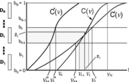
Fig. 1. General formulation of histogram-based quantization (HQ).
II. HISTOGRAM-BASEDQUANTIZATION(HQ)
A. General Formulation of HQ
The concept of HQ is to perform quantization of a feature parameter at time based on the histogram or order statis-tics of that feature parameter within a moving segment of the
most recent past samples, ,
up to the time being considered [23]. As shown in Fig. 1, the values of these parameters in are sorted to produce a time-varying cumulative distribution function , or his-togram, which changes for every time instant , where
and and are, respectively,
the minimum and maximum values within . Also shown in
Fig. 1, partition cells, ,
to-gether with their corresponding representative values,
, are defined on the vertical scale [0, 1], which are derived from a standard Gaussian with cumulative dis-tribution via the Lloyd–Max algorithm [24], [25]. Note
that the boundaries on the vertical scale
can be either uniformly or nonuniformly distributed [23]. In the case of nonuniform quantization, the Lloyd–Max algorithm can be performed with respect to any distribution, including the dis-tribution of training sets. Since different training sets may have different distributions, we performed the Lloyd–Max algorithm based on uniform, Laplacian and Gaussian distributions in the preliminary experiments. The best performance was obtained with Gaussian distribution under noisy environments, probably because the distribution of feature parameters under noisy envi-ronments on the vertical scale is closer to a Gaussian distribu-tion. Using the dynamic histogram constructed with ,
these partition cells on the vertical scale, ,
are then transformed to the horizontal scale to be the
parti-tion cells on the horizontal scale for
the quantization of , where . In other words, the partition cell on the horizontal scale is obtained from the partition cell on the vertical scale via the dy-namic histogram . Thus, the partition cell on the horizontal scale is dynamic. However, the representative values
for these partition cells
on the horizontal scale are fixed, and are trans-formed from the representative values
previously obtained on the vertical scale by the histogram of the standard Gaussian.
The above formulation indicates that HQ is based on a hidden
codebook derived from a standard
by a dynamic histogram into time-varying partition
cells , and by a fixed histogram into the fixed
representative values , both on the horizontal scale. The quantization here is then similar to all conventional quantiza-tion processes, in that it is a mapping relaquantiza-tion which maps the present parameter to a fixed representative value , if is within the partition cell , except that this partition cell is dynamically defined
if or
(1) Note that the quantization codebook here includes a set of
dy-namic partition cells and a set of
fixed representative values . It will be
shown below that many practical problems mentioned previ-ously can be automatically solved to a good extent in this way. Also, although here HQ is a quantization process, it can also be used as a feature transformation process offering the desired robustness as will also be discussed below, in which each pa-rameter is transformed to its representative value for the corresponding partition cell.
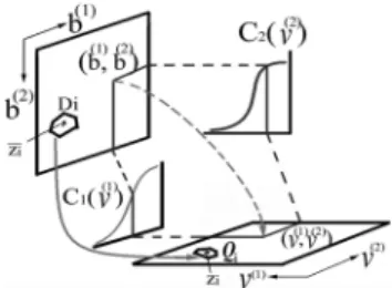
B. Histogram-Based Vector Quantization (HVQ)
The above general formulation of one-dimensional HQ in Fig. 1 can be easily extended to HVQ with more than one dimension. Consider SVQ as an example [4], in which two MFCC parameters (e.g., and ) can be quantized jointly by a two-dimensional VQ codebook. Extending from the one-dimensional HQ mentioned above, a moving segment of the most recent past samples of the first parameter up
to time , , gives a histogram
for , and a similar segment of the past samples of the second parameter up to time , , gives another
histogram for . The formulation below is exactly
the same as the one-dimensional HQ in Fig. 1, except that here both the vertical and horizontal axes are no longer one-di-mensional axes, but are extended to vertical and horizontal two-dimensional planes as shown in Fig. 2. On the vertical plane with coordinates , we have a two-dimensional
hidden codebook , which is derived
from a bivariate standard Gaussian via the LBG algorithm [26].
Every point on this plane is then transformed by
the above-mentioned dynamic histograms
back to a point on the horizontal plane, where
. The set of all these points on the horizontal plane transformed from those points on the vertical plane in a certain partition cell then forms the dynamic partition cell on the horizontal plane as follows:
if
(2) On the other hand, the representative points for each partition cell on the vertical plane are similarly transformed back to the fixed representative points on the horizontal plane, except that the transformation is performed by two fixed histograms
Fig. 2. Concept of histogram-based vector quantization (HVQ) using two dimensions.
, , both derived from a one-dimensional stan-dard Gaussian. The quantization here is a mapping relation just as one-dimensional HQ in (1), which maps the present param-eter set to a representative value for the dynami-cally defined partition cell
if
or (3)
Based on the above, the two-dimensional HVQ can be
per-formed dynamically on the plane. For the present
parameter pair at time , the two dynamic histograms
and based on and give a point
on the vertical plane. The partition cell on the vertical plane to which this point belongs then determines the partition cell and representative point on the horizontal plane.
C. Discussions About Robustness of HQ (and HVQ)
Conventionally, feature quantization is for data compression and robust features are for handling noise disturbances. The pro-posed HQ, however, includes the desired robustness in the quan-tization process.
1) Robust Nature of HQ: With the conventional SVQ, the
mismatch between the pretrained fixed VQ codebook and the current corrupted testing features may significantly increase quantization distortions. With the proposed HQ, however, the actual partition cells are dynamically adjusted according to local statistics. For example, as shown in Fig. 1, may be changed to when disturbances are encountered. The partition cell on the horizontal scale for the disturbed parameter
may also be changed to , where
and , which can be quite different from .
Nevertheless, the partition cell and the corresponding rep-resentative value for may remain unchanged as long as , since is fixed on the vertical scale, while the disturbances from to are on the horizontal scale, and is fixed on the horizontal scale. Since the actual partition cells are no longer fixed as in conventional SVQ methods, the codebook mismatch problem mentioned above can thus be avoided to some extent. In other words, HQ is based on the partition cells fixed on the vertical scale and the dynamic histogram , and is therefore less sensitive to disturbances on the horizontal scale: disturbances on the horizontal scale are actually absorbed by the dynamic histogram to a certain degree. When a segment of parameters are corrupted by
small disturbances, all individual values may be changed ( is disturbed into ), but the order statistics which produce the partition cells on the horizontal scale may remain similar, and the representative values remain fixed; therefore, the changes to the quantization results may be very limited. Such robustness is obtained by local order statistics for the most recent past values of feature parameter. This is why HQ is able to handle various noise conditions as will be shown in the experiments presented below.
2) Comparison With Histogram Equalization (HEQ): The
popularly-used HEQ equalizes the cumulative distributions (or histograms) of both the training and testing feature parameters in each temporal span, and has been shown to produce very robust features for recognition [8]–[10]. HQ actually borrows the concept from HEQ. The experiments below will show that HQ can be used as an attractive feature transformation approach for robustness purposes as well, and it even performs better than HEQ. It is important to explain why. HEQ actually per-forms point-to-point feature transformation based on the order statistics, which can absorb the small disturbances to a good degree, although some residual disturbances inevitably remain because the point-based order statistics are in any case more or less disturbed. Quantile-based HEQ [27] performs a piece-wise-linear approximation of HEQ. It reduces the computation complexity for histogram estimation, but does not change the point-based nature of the transformation. HQ, on the other hand, performs the transformation block by block; therefore, the small disturbances within each block ( in Fig. 1) are absorbed by the block-based order statistics. The block-based order statis-tics certainly introduce uncertainty as well, but with the proper choice of the number of quantization levels or the block size, this uncertainty may be compensated for by the stochastic nature of the Gaussian mixtures in the HMMs. HEQ can be considered the limiting case of HQ when the number of quantization levels becomes infinite. As will be shown below, the recognition performance certainly depends on the value of considering the noise conditions and so on, but being infinite is not nec-essarily the best.
III. JOINTUNCERTAINTYDECODING(JUD)FORHQ Uncertainty decoding has been developed for HMM decoding considering the uncertainty of the observation vectors. Such techniques are also very useful for the HQ developed here, as presented below.
A. General Formulation of Uncertainty Decoding
In standard HMM decoding, the probability for ob-serving a feature vector at a state is
(4)
where is the mixture index, and are,
respec-tively, the mixture weight, mean, and covariance for the th Gaussian mixture in state . There have been slightly different approaches in formulating the concept of uncertainty decoding [12], [14]. In the approach used here [3], [13], [15], instead of evaluating the observation probability only for a single
feature vector , uncertainty decoding treats the observed fea-ture vector as being corrupted, and therefore considers the un-corrupted but unobservable feature vector as a random variable with a distribution during decoding. The probability of observing , , can then be defined as the expected value of with respect to the distribution [3], [13], [15]
(5)
Assuming to be Gaussian with mean and
covari-ance matrix , , where both
and can be estimated in various ways, the integration in (5) can be reduced to [13]
(6) Thus, the standard HMM decoding using (4) remains un-changed, except that the variance of each Gaussian in the HMMs is increased by , the uncertainty of the unobserv-able vector . In this way, the Viterbi decoding can be based more on reliable parameters with a smaller variance . The observed feature vector can be taken as the estimated value of for simplicity, as is done here in this section. However, can also be estimated based on previous feature vectors as in the three-stage error concealment approaches as discussed later on. Below, we present the approaches used here to estimate the uncertainty of the unobservable feature vector
, or the covariance matrix .
B. JUD for HQ
There are two sources of uncertainty in HQ-based features: quantization errors and environmental noise. Here, we first sep-arately estimate them and then consider them jointly.
1) Quantization Error Uncertainty: In an HQ partition cell,
the representative value is the observed corrupted feature vector in (5), and all the possible samples in the corresponding th partition cell are these samples for the uncorrupted unquantized feature vectors in (5) collected at the client, which are unobservable at the server. The variance for quantiza-tion errors in the th partiquantiza-tion cell to be used to take the place of in (6) can thus be estimated using a clean speech training set. Taking the one-dimensional HQ as in Fig. 1 as an example
(7) where the summation is over all feature parameters in the th partition cell in the training set. Equation (7) can be easily extended to HVQ for more dimensions. Because the representative value was obtained via the Lloyd–Max algo-rithm (or LBG algoalgo-rithm [26] in the case of HVQ) based on the histogram for a standard Gaussian distribution, all param-eters in the partition cell need to be transformed first by
then transformed back via to evaluate . Because
the Lloyd–Max algorithm produces tightly quantized levels in high-density regions and loosely quantized levels in low den-sity regions to minimize total distortion, uncertainty decoding automatically increases the Gaussian variances for the loosely
TABLE I
AVERAGEDHISTOGRAMSHIFT FORHQ UNDERDIFFERENTSNR CONDITIONS
quantized levels. In this way, can be trained in advance for
all partition cells .
2) Environmental Noise Uncertainty: Under low SNR
conditions, disturbances may be very serious. For example, in
Fig. 1, and may be changed to and and to
, or there may be a histogram shift which cannot be well absorbed by the dynamic histogram. Inevitably, then, HQ’s performance deteriorates. Such a histogram shift may be
rea-sonably estimated by , because for a
standard zero-mean Gaussian. For server-side histograms con-structed based on the quantized codewords, the average values
of under all types of noise for the AURORA 2
testing environments (with further details in Section V) for dif-ferent SNR values are shown in Table I. Clearly, the histogram shift increases with lower SNR values. This is reasonable because under lower SNR conditions, the order statistics and histograms of the original speech samples collected at the client in the respective moving segments change very rapidly; thus, the quantized HQ codewords based on these histograms also change quickly and significantly with time. As a result, the server-side histogram constructed using the quantized HQ codewords also change quickly and significantly with time, introducing a significant and fast fluctuating bias or shift in each short segment, even if the original noise added to the signal samples is zero-mean in the long term. Hence, we can take the histogram shift as a simple indicator for the SNR condition: that is, higher such shifts correspond to lower SNR values. Therefore, the variance for uncertainty caused by environmental noise at time —used in place of in (6)—can be reasonably estimated as
(8) where is an empirically determined scaling factor and is fixed for all SNR values and noise conditions in our experiments. In fact, the value of only indicates the relative importance of feature parameters in Viterbi decoding—we found in prelimi-nary experiments that recognition performance is not very sen-sitive to the value of chosen here. is the histogram for the HQ-quantized codewords for all feature parameters in the moving segment at frame . In this way, in the DSR case, can be estimated at the server easily for each time without any extra bit rate costs. This allows us to solve the problem where the environmental disturbances are hidden in codewords and cannot be estimated directly.
3) Joint Uncertainty Decoding (JUD) for HQ: The above
two types of uncertainties should be jointly considered [28]. A reasonable assumption is that for higher SNR conditions the quantization error uncertainty dominates, while for lower
SNR conditions, the environmental noise uncertainty dom-inates. Therefore, the joint uncertainty for a codeword in the th partition cell at time can be estimated as
(9) where is pretrained for the th partition cell using (7), and is estimated in real time using (8). This value of can then be used as directly in (6).
C. Histogram-Shift Compensation
As mentioned previously, histogram shift occurring at lower SNR values inevitably results in seriously degraded HQ perfor-mance. As a result, in addition to the uncertainty decoding as mentioned above, we can also shift the histogram horizontally to have
(10) for each time . A large portion of the serious disturbances can be absorbed by such a shift, as will be verified by the experi-ments below.
IV. THREE-STAGEECFORHQ-BASEDDSR SYSTEMS Here, we consider the approaches to handling the transmis-sion errors added to the received HQ codewords under the DSR framework [29]. A three-stage EC approach is developed, as presented below.
A. Stage 1—Error Detection
In the ETSI DSR standards, every two frames are grouped together and protected with four-bit CRC [4]. In this way, the entire frame-pair is labeled erroneous even if only a single bit error occurs in the frame-pair packet. Adding check bits at the subvector level is helpful for subvector level error detection, but comes at the cost of additional bandwidth [7]. A more ef-ficient way is to make use of the speech signal characteristics at the subvector level. The data consistency test checks the con-tinuity of the parameters in two neighboring subvectors [21]. When the difference between two consecutive values of a fea-ture parameter in a subvector exceeds a predetermined threshold obtained from some training corpus, the subvector is classified as inconsistent. However, if the statistics of the testing features are time-varying and different from those of the training corpus, this approach becomes less reliable. With environmental noise, the parameters are likely to be classified as inconsistent even if they are correctly received.
HQ performs feature parameter quantization based on the local histogram (or order statistics), so the quantized codewords represent the local order-statistic information of the original pa-rameters. The quantization process does not change the order statistics of the parameters, and if there are no transmission er-rors, the histogram for the subvector codewords received at the server should be similar to the histogram for the original fea-ture parameters at the client. Thus, the partition cell obtained by reperforming HQ on the received subvector codeword, based on the dynamic histogram for these received codewords, should
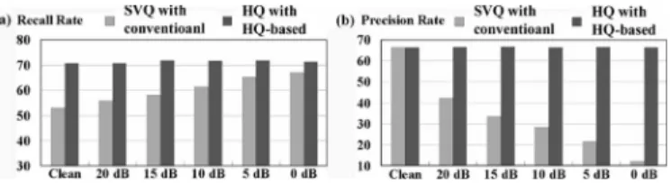
Fig. 3. (a) Recall and (b) Precision rates for error detection using SVQ with the conventional data consistency check and HQ with the HQ-based consistency check proposed here.
be the original partition cell. If not, it is very possible that the order statistics have been changed and the received subvector codeword may be erroneous. Based on this observation, the consistency test in the HQ framework proposed here is as fol-lows. Taking a two-dimensional HVQ as an example,
is a received subvector codeword at some time, and represents the representative value for the sub-vector assigned by HQ performed at the server based on the histogram for the received codewords. The subvector
is then classified as consistent if
(11) In other words, if these two parameters are correctly received, their order statistics at the server should be similar to the order statistics for the original values before quantization at the client, and therefore similarly quantized into the same HQ partition cell.
We compared the error detection accuracy of the conven-tional SVQ scheme with the data consistency check [21] and the proposed HQ with the HQ-based consistency check mentioned above under all different noise conditions for the AURORA 2 testing environment with the transmission errors introduced by the General Packet Radio Service (GPRS) wireless environment (further details are presented in Section V below). The averaged recall (percentage of detected errors out of all errors) and preci-sion (percentage of correct errors out of all detected errors) rates for error detection are shown in Fig. 3(a) and (b). For lower SNR cases, it is clear that the noise seriously affects the SVQ with data consistency check as verified by the precision degradation in Fig. 3(b) (from 66% at clean down to 12% at 0 dB). With the proposed HQ-based consistency check approach, however, the precision rate is much more stable at all SNR values, and both recall and precision rates are higher.
Note that when (11) is not satisfied, it is also possible that the present codeword is actually correctly received, but instead the dynamic histogram, on which the HQ in (11) is based, is dis-turbed by erroneous received codewords in the past frames. This is one good reason why the precision rate in Fig. 3(b) for HQ with the proposed consistency check is slightly less than 70%, i.e., some detected inconsistencies are actually correctly received codewords. However, this precision is much higher than SVQ with conventional approach. In fact, the probability that the inconsistency in (11) is due to the disturbed histogram rather than the considered codeword being erroneous is lower, because the effect of the erroneous codewords in the past frames is reasonably absorbed by the histogram (the order sta-tistics of a large number of codewords) as well as the partition
cells in HQ. In other words, with erroneous codewords in the past frames, the change of the histogram may not be very serious, and the partition cell that the present codeword being considered belongs to may remain unchanged. This is verified in Fig. 3(b) where the precision rate, although much less than 100%, remains almost the same from clean speech to 0-dB SNR.
B. Stage 2—Erroneous Feature Vector Estimation
Different techniques for estimating the detected erroneous feature vectors have been proposed. Repetition and interpola-tion only use the correctly received feature vectors [16], while statistical-based techniques use prior knowledge about speech source in addition, and have been shown to offer better perfor-mance [30].
The erroneous subvector estimation proposed here under the HQ framework is based on the maximum a posteriori (MAP) criterion, which determines the estimated value of a certain transmitted subvector codeword at time , which is detected as erroneous (here both and are certain codewords men-tioned above for some , respectively). This MAP estimation is conditioned on the present and previously received
corre-sponding subvector codewords and (here both and
are also certain codewords mentioned above for some , respectively)
(12)
where denotes that is the th HQ codeword out of
the possible codewords. The maximization here is over all of these codewords. If we assume and are independent
(13) With the denominator in (13) left out in the maximization in (12), the probability in (12) can be approximated by the
code-word bigram and the channel transition
prob-ability
(14)
In (14), the codeword bigram can be
esti-mated by the bigram of the considered subvector codewords trained from a clean training set (for example, the clean training set of AURORA 2). Also, the channel transi-tion probability in (14) can be estimated from the bit error rate (BER) of the present frame being considered
(15) where BER is estimated as the total number of inconsistent subvectors (in simulation analysis, it was found that in most cases there is only one bit error in an erroneous codeword, and therefore this number can be used to estimate the total number of erroneous bits) detected in the first stage (discussed in Section IV-A) in the present frame divided by the total number of bits in the frame, is the total number of bits in the
received subvector codeword , and are,
respec-tively, the bit patterns for the codewords and , and represents the Hamming distance between two bit patterns.
TABLE II
MUTUALINFORMATIONI(s ; s )FORSVQANDHQ
The value of in (15) is actually the probability
of being changed to if BER can be accurately estimated. With (15), when is less reliable (or has a larger BER), the
values of for all possible codewords with
different become closer to each other (i.e., the difference in is insignificant for different Hamming distances ). On the other hand, when is more reliable (or has a
smaller BER), is larger for only few values of .
In this way, more emphasis can be put on the codeword bigram than on the channel transition probability in (14) when the channel condition is less reliable.
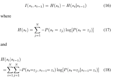
Because the basic principle here is to exploit the short-time correlation between consecutive frames in speech signals to es-timate the lost subvectors, the robustness of HQ as mentioned in Section II-C is very helpful. If the quantization process is less robust, the environmental noise may move the feature vectors to a different partition cell and the subvector transition relation-ship in speech signals may be disturbed. This problem is actually lessened by the HQ’s robustness, as can be verified by the mu-tual information between the present and previous subvector codewords and
(16) where
(17)
and
(18)
are, respectively, the degree of uncertainty for the present sub-vector , and the remaining degree of uncertainty for after the previous subvector is known. Thus, the mutual
infor-mation in (16) shows how much the codeword
bi-gram model reduces uncertainty for the subvectors . In other words, a bigram model with higher mutual information implies that predicting the present subvector given the previous sub-vector is easier. The mutual information for the conven-tional SVQ and the proposed HQ averaged for different subvec-tors from the three testing sets of AURORA 2 is listed in Table II. We can see that HQ’s mutual information is always higher than that of SVQ, which indicates that the HQ framework allows for more precise estimation of the lost subvectors.
C. Stage 3—Uncertainty Decoding
The uncertainty decoding discussed in Section III-A can be used here in the final stage. Consider Section III-A: the above received codeword is taken as the observed corrupted fea-ture vector in (5), and all of the possible transmitted
code-words, , , are the possible samples of
the uncorrupted but unobservable feature vector in (5). The
distribution of the probability obtained in
(12) then characterizes the uncertainty of the observed code-word. With the estimated codeword in (12) taken as the mean and the covariance estimated using the probability
distri-bution taken as the covariance , both
used in (6), uncertainty decoding can then be directly performed within the HQ framework as presented previously by increasing the variance of each Gaussian mixture by in the HMMs as in (6) [28]. In this way, HMM decoding puts more emphasis on more reliable subvectors, i.e., those with lower covariance
for the probability distribution in (12).
D. Three-Stage EC Under the HQ Framework
The three stages of EC under the HQ framework can be easily integrated. At the first stage, the received frame-pairs are first checked with CRC to detect errors at the frame level. The erro-neous frame-pairs are then further checked at the subvector level by the HQ consistency test as mentioned in Section IV-A. At the second stage, the erroneous subvectors detected at the first stage are estimated and reconstructed as presented in Section IV-B. At the third stage, uncertainty decoding in the Viterbi search process makes the HMMs less discriminative for subvectors with higher uncertainty as presented in Section IV-C.
V. EXPERIMENTALCONDITIONS
All the experiments reported in this paper were conducted on the AURORA 2 testing environment [22] based on a corpus of English connected digit strings. Two training conditions (clean-condition and multicondition) and three testing sets (sets A, B, and C) were defined in AURORA 2. Both clean and noisy speech signals were prepared by filtering the TI database (both training and testing) using a telephone-bandwidth bandpass filter. The testing set A included four types of noise which were used in the multicondition training (subway, babble, car, and exhibition), while the testing set B included another four types of noise not used in the multicondition training (restaurant, street, airport, and train station). The testing set C was filtered with a MIRS (Modified Intermediate Reference System, which simulates the bandpass filtering [300–3400 Hz] behavior of the telephone channels in the public switched telephone networks [PSTN]) characteristic filter [22], [31] before adding two ad-ditive noise types (subway in set A and street in set B). In all sets A, B, and C, the SNR tested ranged from 20 to 5 dB. The MFCC extraction follows the WI007 front-end [22] defined in AURORA 2 with frame length 25 ms and frame shift 10 ms, which gives 13 coefficients (C1-C12 and log energy) to be used to obtain the delta and delta-delta features together for recognition.
General Packet Radio Service (GPRS) was chosen in this re-search as an example for wireless channels in the experiments;
GPRS was developed by ETSI based on a packet switching framework to enhance the GSM system. GPRS shares the GSM frequency bands and uses several properties of the physical layer of the GSM system. It includes four different error control coding schemes, CS1-CS4, each with a different code rate. The GPRS simulation software used in the tests described here was developed by the Wireless Communication Laboratory of National Taiwan University [32], in which all complicated transmission phenomena have been carefully simulated in de-tail, such as the propagation model, multipath fading, Doppler spread, etc. The experimental results presented below are based on the following simulation configurations: typical urban (TU, an environment more frequently encountered with a more severe fading problem), the client traveling at speeds of 3, 50, 100, 250 km/h, single antenna, hard decision at the receiver, and CS4 (i.e., without any protection) coding scheme, which corresponds to a transmission bit error rate of 5.3% for a client traveling at a speed of 3 km/h.
VI. EXPERIMENTALRESULTS
The fundamental experimental results for HQ as dis-cussed in Sections II-A–C are briefly reported in sections Sections VI-A–C. Sections VI-D and VI-E then present the results for robust and distributed speech recognition systems, respectively. All the experiments reported here were based on order statistics over segments of most recent past parameter values as mentioned in Section II, so there was no time delay. Better results were obtainable if this no-delay condition was removed.
A. HQ as a Feature Transformation Method
In the first set of experiments, we considered the case of ro-bust speech recognition apart from the DSR environment, in which one-dimensional HQ was used as a feature transforma-tion technique, that is, each feature parameter is transformed to the representative value for the corresponding partition cell as in (1) to be used for recognition.
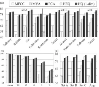
The results are shown in Fig. 4(a)–(c). The recognition ac-curacies for baseline experiments with original MFCC features, compared to those with MFCC parameters filtered by the MVA filter (mean and variance normalization followed by autoregres-sion moving-average (ARMA) filtering) [33] and the principal component analysis (PCA) filter derived [34], as well as trans-formed by the well-accepted HEQ [8]–[10], and the proposed one-dimensional HQ are, respectively, shown in Fig. 4 under clean-condition training for (a) averaged over all SNR values but separated for different types of noise, (b) averaged over all types of noise but separated for different SNR values, and (c) averaged over all types of noise and all SNR values for testing sets A, B, and C, respectively. Here, the order of the MVA filter was , the PCA filter was performed with filter length , and HEQ was performed in exactly the same way as HQ, based on a moving segment of the most recent past pa-rameters, and the same value of (or one second) was used for all experiments for both HEQ and HQ. It has been ver-ified that long-term features derived from one second time in-terval carry important speech information [35].
Fig. 4. Accuracies for MFCC baseline and those transformed by MVA filtering, PCA filtering, HEQ, and HQ, respectively, under clean condition training. (a) Averaged over all SNR values but separated for different types of noise. (b) Averaged over all types of noise but separated for different SNR values. (c) Averaged over all types of noise and all SNR values for different testing sets.
Many observations can be made here. First, it is clear that HQ (the last bar) significantly improved the performance as compared to the baseline MFCC (the first bar) for all testing sets, all SNR values (except for the clean speech case), and all noise types. For example, from Fig. 4(a), it can be observed that for speech-like noise such as babble or restaurant noise, the MFCC baseline accuracy (around 50%) was much lower as compared to most other noise types (around 60% or more). HQ was able to absorb the speech-like variation and improved the performance in such a way that the results for different noise types were not only much higher, but also were more similar to each other (around 80%). As another example, in Fig. 4(b) the recognition accuracy of HQ was 87.88% as compared to MFCC baseline 66.95% at 10-dB SNR. The improvements be-came even more significant for lower SNRs. Second, HQ pro-posed here performed consistently better than MVA, PCA, and HEQ compared here for all testing sets, all noise types, and all SNR conditions (except for clean speech cases). In particular, HEQ and HQ (the fourth and fifth bars) performed better as compared to MVA and PCA (the second and third bars). This is probably because HEQ and HQ dynamically transform the MFCC features considering the whole distribution locally, while the filters used in MVA and PCA are fixed, and only the first and second moment statistics are taken into consideration. Fur-thermore, in all Fig. 4(a)–(c), HQ performed consistently better than HEQ for all testing sets, all noise types, and all SNR con-ditions. For example, in Fig. 4(a), HQ turned out to be very helpful for babble/restaurant noise (78.41%/79.08%) as com-pared to HEQ (75.95%/76.28%), probably because in such cases of speech-like noise, the order statistics disturbances were better absorbed by HQ’s blocks than by HEQ’s point-by-point trans-formation. For subway noise, on the other hand, the improve-ment of HQ (81.70%) compared to HEQ (80.86%) is relatively less, probably because the impulse-like disturbances may very often exceed beyond the blocks.
TABLE III
AVERAGEDNORMALIZEDDISTANCESBETWEENCLEAN ANDCORRUPTEDSPEECHFEATURESUNDERDIFFERENT
SNR VALUES FORHEQANDHQ (1-D)
We further compared HEQ with HQ (one-dimensional) tested here using a different metric, the averaged normalized distance between the corrupted feature parameters and the corresponding clean speech feature parameters
(19) where the average in (19) is performed over all feature param-eters in all the testing speech in sets A, B, C, is the total number of frames, and is the standard deviation for all the clean feature parameters . Both and have been pro-cessed by either HEQ or HQ, so the difference ( ) indicates how the mismatch caused by noise disturbance is reduced by ei-ther HEQ or HQ for each individual feature parameter. Smaller values of imply that the features are less influenced by dis-turbances, although is not necessary directly related to recog-nition accuracy. The results are listed in Table III for different SNR values. We find in the table that the values of consistently increase as the SNR value degrades, which makes very good sense, and HQ clearly gives smaller values of in all cases. This may explain from a different perspective why HQ performed better than HEQ.
B. HQ as a Feature Quantization Method
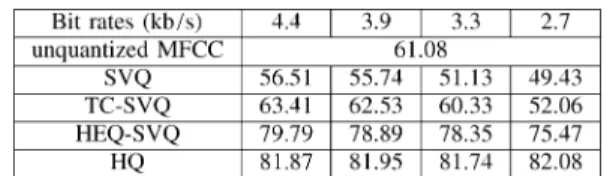
The next set of experiments considered HQ as a feature quantization method in a DSR framework. However, here we first examined the effect of quantization and compression on recognition accuracy, so we assume that the environmental noise was present with the input speech, but there were no transmission errors. For comparison, recognition accuracies for MFCC features with quantization and compression using the standard SVQ [4], the well-known transform coding [5], [7] (i.e., performing quantization in the transformed domain) followed by SVQ (TC-SVQ), the cascade of the HEQ front-end with SVQ (HEQ-SVQ), and the proposed HQ (actually two-di-mensional HVQ) for bit rates 4.4, 3.9, 3.3, and 2.7 kb/s are listed, respectively, in Table IV for clean-condition training, av-eraged over all ten types of noise and all SNR values in sets A, B, and C. The recognition accuracies for baseline experiments with original MFCC features without quantization is 61.08%. Because all these results are averages over all SNR values from 20 down to 0 dB, the numbers here are not very high. Note that the performance of HQ was consistently and significantly better than SVQ, TC-SVQ, and HEQ-SVQ under all transmission bit rates. For example, at bit rate of 2.7 kb/s, the overall accuracy of HQ (82.08%) represented relative error rate reductions of 26.93%, 62.62%, and 64.57%, respectively, as compared to those with HEQ-SVQ (75.47%), TC-SVQ (52.06%), and SVQ (49.43%). It is even significantly higher (with an error rate reduction of 53.96%) than the original unquantized MFCC
TABLE IV
RECOGNITIONACCURACIES FORFEATUREQUANTIZATION ANDCOMPRESSION
WITHCLEAN-CONDITIONTRAINING, AVERAGEDOVER ALLSNR VALUES AND
NOISETYPES INSETSA, B,ANDCFORDIFFERENTBITRATES(4.4TO2.7 kb/s)
(61.08%). This was clearly due to the robust nature of HQ, as discussed previously. Note that the original uncompressed MFCC degraded seriously under noisy conditions, but HQ held up quite well. Also note that the performance of SVQ, TC-SVQ, and HEQ-SVQ all degraded significantly under lower bit rates, while the performance of HQ remained very stable for different bit rates, or the performance of HQ is actually relatively insensitive to the quantization resolution in (1). These results indicate that, with the conventional distance-based quantization (SVQ), even with the more robust feature transformation front-end (TC or HEQ), the quantization distortion and environmental noise still jointly degraded the performance seriously. The HQ approaches, however, were able to reconstruct the feature parameters based on the order statistics or histogram, which automatically absorbed many of the disturbances, therefore offering a much better recognition accuracy.
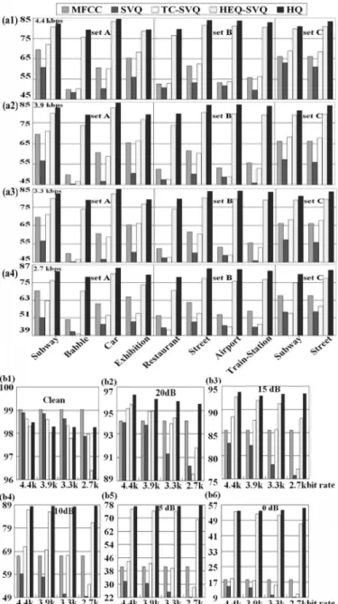
The results in Table IV are averaged over all SNR values and all noise types in sets A, B, and C. Further, we see in Fig. 5(a1)–(a4) the detailed accuracies obtained in exactly the same experiments, but separated for different noise types and averaged over all SNR values for different bit rates (4.4, 3.9, 3.3, and 2.7 kb/s), respectively. From Fig. 5(a1)–(a4), we can find that HQ (the last bar in each set) consistently performed much better than the other approaches compared in Table IV (the first four bars in each set). HQ can even handle nonstationary disturbances as well to a good degree, clearly because it is based on the dynamic histogram of the most recent past values. For example, in the case of 3.3 kb/s in Fig. 5(a3), HQ is actually significantly better than HEQ-SVQ (78.82% versus 73.69%, 79.40% versus 73.77%, 83.80% versus 79.37%, and 83.12% versus 77.82% for babble, restaurant, airport, and train-station noise cases, respectively), and the corresponding numbers for MFCC, SVQ, and TC-SVQ approaches were much lower.
C. Further Analysis of Bit Rates Versus SNRs for HQ as a Feature Quantization Method
To see how quantization distortion (or bit rate) mixed with the environmental noise (SNR) in the input speech jointly influences the recognition performance of a DSR system (as-suming no transmission errors), the respective accuracies for the same experiments mentioned in Section VI-B and listed in Table IV are further analyzed, respectively, for different bit rates and different SNRs as shown in Fig. 5(b1)–(b6) for clean to 0-dB SNR. For clean speech, SVQ performed the best (although slightly lower than unquantized MFCC) under higher bit rates (4.4, 3.9, and 3.3 kb/s), while for other approaches (TC-SVQ, HEQ-SVQ, and HQ) feature transformation more or
Fig. 5. Recognition accuracies for feature quantization and compression with clean-condition training. (a1)-(a4) Averaged over all SNR values but separated for different types of noise at bit rates of 4.4 to 2.7 kb/s. (b1)-(b6) Averaged over all types of noise but separated for different bit rates (4.4 to 2.7 kb/s) at different SNR values.
less changed the speech characteristics, and therefore inevitably slightly degraded the performance for clean speech. At a lower bit rate such as 2.7 kb/s, however, HQ offered better perfor-mance than other approaches. This is probably because SVQ is more sensitive to quantization distortion, so the performance of SVQ, TC-SVQ, and HEQ-SVQ all degraded for lower bit rates. On the other hand, the dynamic nature of HQ makes it relatively insensitive to the quantization resolution (or bit rates), as can be verified in the clean speech case in Fig. 5(b1). Under noisy environments (SNR from 20 dB all the way down to 0 dB), HQ consistently performed better than other approaches for all SNR values and all bit rates. Under very poor SNR conditions, the noisy disturbances were very serious, but still well absorbed by the HQ histogram. For example, in the case
of 5-dB SNR and 2.7 kb/s bit rate, HQ offered an accuracy of 77.61% compared to 22.30% for SVQ, 28.31% for TC-SVQ, and 69.07% for HEQ-SVQ. HQ offered an accuracy of higher than 50% (55.27%) even at 0-dB SNR and the low bit rate of 2.7 kb/s. These results indicate that for SVQ the mismatched codebooks significantly increase the quantization distortion, especially under poorer SNR conditions. The performance of HQ, however, remains relatively high and even very stable for different bit rates for SNR degrading from 20 to 0 dB. This verified that HQ is very robust against both quantization distortion and environmental noise.
D. HQ-Based Robust Speech Recognition System With Joint Uncertainty Decoding (JUD)
Here, we consider a complete HQ-based robust speech recog-nition system under noisy conditions, outside of the DSR or client-server framework. The input speech features were first transformed by HQ just as was presented in Section VI-A. In ad-dition, in this section JUD as discussed in Sections III-A–III-C was further applied at the decoder, including the histogram shift plus the uncertainty estimated for the environmental noise and quantization errors.
The results are plotted in Fig. 6. Note that in Fig. 6(b) the plots for 5- and 0-dB SNR are shown in different scales so as to make the differences easier to observe. The four bars in each set in Fig. 6(a)–(c) are, respectively, for the accuracies obtained with the proposed HQ feature transformation alone (one-dimen-sional with bit rate (resolution) 3.9 kb/s, exactly the same as the last bar in Fig. 4 presented in Section VI-A), HQ plus histogram shift (HQ-s, Section III-C), HQ with histogram shift plus un-certainty for environmental noise (HQ-s,n, Sections III-C and III-B2), and HQ with complete JUD including histogram shift and uncertainty for environmental noise and quantization er-rors (HQ-s,n,q, Sections III-C and III-B). It can be found in Fig. 6(a)–(c) that with the various JUD approaches proposed in Sections III-B and III-C performed at the decoder, accuracies can be consistently improved step-by-step in all cases. There was almost no performance degradation for clean speech, and slight improvements at high SNR conditions [Fig. 6(b)]: this implies uncertainty decoding for HQ is able to preserve the discrimination among HMMs. In other words, it is clear that the quantization process produces quantization errors, but with proper design of the quantizer and the uncertainty decoding, quantization errors and environmental disturbances can in fact be well absorbed and compensated for to a good extent. Accu-racies for the first and the last bars in Fig. 6(c) (HQ alone and HQ-s,n,q with complete JUD) are also compared in Table V. It can be found that significant error rate reduction was actually achieved in all three testing sets.
E. HQ-Based Distributed Speech Recognition (DSR) System
Here, we finally consider a complete DSR system based on the proposed HQ approaches. HQ was first applied at the client end to quantize and compress the input speech features. The quantized codewords were then transmitted via wireless net-works to the server. JUD discussed in Section III was then ap-plied at the server to improve accuracies. There were inevitable
Fig. 6. Performance improvements obtained by the various JUD approaches as compared to HQ alone: (a) averaged over all SNR values but separated for different noise types in sets A, B, and C. (b) Averaged over all noise types but separated for each SNR value. (c) Averaged over all SNR values and noise types but separated into sets A, B, and C.
TABLE V
ACCURACIES ANDERRORRATEREDUCTIONS FORHQ ALONE
(ONE-DIMENSIONAL, 3.9 kb/s)ANDHQ-s,n,q (WITHCOMPLETEJUD)
FORDIFFERENTTESTINGSETS INFIG. 6(c)
transmission errors introduced by the wireless channels, and the three-stage EC discussed in Section IV was finally applied.
1) HQ-JUD Compared With Conventional Approaches As-sociated With SVQ, But Without Transmission Errors: Before
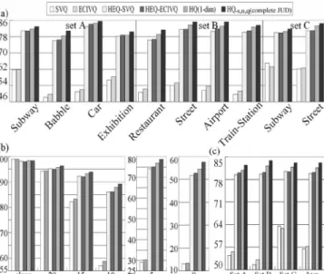
considering transmission errors, the first issue to be investigated here is feature quantization and compression. Conventionally, in DSR this is done using SVQ [4]. If noise can be properly handled to a good degree by cascading an HEQ process at the front, we can also compensate for quantization errors caused by SVQ using some conventional approaches associated with SVQ, for example the well-known extended cluster informa-tion vector quantizainforma-tion (ECIVQ) [3]. Therefore, we need to compare the proposed HQ followed by JUD with such conven-tional approaches associated with SVQ first. The results are in Fig. 7(a)–(c). The six bars in each set in Fig. 7 are, respectively, for SVQ alone, ECIVQ alone, the cascade of HEQ front-end and SVQ (HEQ-SVQ), the cascade of HEQ front-end and ECIVQ (HEQ-ECIVQ), HQ (two-dimensional), and the same HQ with complete JUD including histogram shift (HQ-s,n,q), all with bit rates 4.4 kb/s. The first, third, and fifth bars in Fig. 7 are the same as the second, fourth, and fifth bars of the first 4.4-kb/s group in Fig. 5.
We can find from Fig. 7 that ECIVQ (second bar) performed better than SVQ (first bar) for sets A and B, but slightly worse for set C, and the same trend can be observed when HEQ is performed as a front-end of SVQ (HEQ-SVQ, third bar versus
Fig. 7. Comparison of different approaches discussed in this paper for DSR. (a) Averaged over all SNR values but separated for different noise types in sets A, B, and C. (b) Averaged over all noise types but separated for different SNR values. (c) Averaged over all SNR values and noise types but separated for sets A, B, and C.
TABLE VI
ACCURACIES ANDERRORRATEREDUCTIONS FORHEQ-ECIVQANDHQ-s,n,q (WITHCOMPLETEJUD)AT4.4 kb/sFORDIFFERENTSNR VALUES INFIG. 7(b)
HEQ-ECIVQ, fourth bar). This is probably because ECIVQ considers quantization errors only, but the channel mismatch for set C might move the feature vectors to different partition cells, for which the cluster variance used in ECIVQ was not able to help. HEQ offered very significant improvements when cas-caded with SVQ or ECIVQ (HEQ-SVQ or HEQ-ECIVQ, third or fourth bar), but the HQ (fifth bar) proposed here consistently provided better performance in almost all cases, and the com-plete JUD proposed here including histogram shift (HQ-s,n,q, sixth bar) offered additional improvements consistently in al-most all cases. The accuracies for HEQ cascaded with ECIVQ (HEQ-ECIVQ, fourth bar) and HQ with JUD (HQ-s,n,q, the last bar) are further compared in Table VI. The relative error rate re-ductions shown in the last row are significant and consistent for all SNR values, including the clean and 20-dB cases.
The above experimental results in Fig. 7 and Table VI are for a 4.4-kb/s bit rate. Further analysis was then performed for sev-eral better approaches found above with respect to different bit rates (4.4, 3.9, 3.3, and 2.7 kb/s) at all different SNR values. The results are shown in Fig. 8(a)–(f) for different SNR from clean to 0 dB, each with different bit rates. The four bars in each set in Fig. 8 are, respectively, for ECIVQ considering quan-tization error uncertainty for SVQ, the cascade of transform coding (TC) and ECIVQ (TC-ECIVQ), the cascade of HEQ and ECIVQ (HEQ-ECIVQ), and HQ with complete JUD in-cluding histogram shift (HQ-s,n,q). Here, except for the clean speech case at higher bit rates, HQ-s,n,q consistently performed
Fig. 8. Comparison of different approaches discussed in this paper for DSR (but without transmission errors) under different bit rates and SNR values. (a) Clean. (b) 20 dB. (c) 15 dB. (d) 10 dB. (e) 5 dB. (f) 0 dB.
Fig. 9. Comparison of SVQ, HEQ-SVQ, and HQ, and those with GPRS trans-mission errors (SVQg, HEQ-SVQg, HQg), averaged over all types of noise, but separated for each SNR value.
better for all SNR values and all bit rates than other combi-nations of the front-end feature transformation (TC or HEQ) or back-end compensation considering quantization uncertainty (ECIVQ). Also, the performance of ECIVQ, TC-ECIVQ, and HEQ-ECIVQ are all more sensitive to lower bit rates, while HQ-s,n,q is relatively insensitive to different bit rates at all SNR conditions.
2) HQ-Based DSR Over Wireless Channels With Transmis-sion Errors, But Without EC: We first compared the
robust-ness of SVQ and HQ against environmental noise at the client end plus the transmission errors at a client traveling speed of 3 km/h, assuming no EC approach was used. Fig. 9 is the av-eraged results over all different types of noise but separated for different SNR values. The first three bars are the results for the standard SVQ, SVQ followed by HEQ front-end (HEQ-SVQ), and HQ (two-dimensional), all at 4.4 kb/s and without trans-mission errors, exactly the same as the first, third, and fifth bars in Fig. 7(b), and the next three bars are those suffering from GPRS transmission errors (SVQg, HEQ-SVQg, HQg: the label “g” indicates GPRS). For SVQ, the performance degradation caused by GPRS (first bar compared to fourth bar) is larger when SNR is lower, even with HEQ (second bar compared to fifth bar, e.g., 98.07% to 87.78% for clean speech, 91.97% to 76.74% for 15-dB SNR, and 85.86% to 68.73% for 10-dB SNR). Clearly,
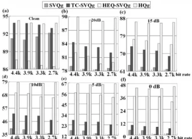
Fig. 10. Comparison of SVQg, TC-SVQg, HEQ-SVQg, and HQg (all with GPRS transmission errors), for different bit rates and SNR values. (a) Clean. (b) 20 dB. (c) 15 dB. (d) 10 dB. (e) 5 dB. (f) 0 dB.
features corrupted by noise are more susceptible to transmis-sion errors. The improvements that HQ offered over HEQ-SVQ when transmission errors were present (sixth bar to fifth bar) are consistent and significant at all SNR values. For example, in the case of 10-dB SNR with GPRS, HQ (sixth bar) offered an ac-curacy of 78.69% while the number was 69.84% for HEQ-SVQ (fifth bar). This verified that HQ is robust against both environ-mental noise and transmission errors.
The above results in Fig. 9 are for a 4.4 kb/s bit rate. Fur-ther analysis was then performed for several better approaches found above with respect to different bit rates (4.4, 3.9, 3.3, and 2.7 kb/s) for all SNR values (from clean to 0 dB) as shown in Fig. 10(a)–(f). The four bars in each set in Fig. 10 are, re-spectively, for SVQg, transform coding followed by SVQ (TC-SVQg), the cascade of HEQ and SVQ (HEQ-(TC-SVQg), and HQg, all with GPRS transmission errors. Here, HQ consistently per-formed better than different versions of SVQ enhanced by some feature transformation approaches (TC or HEQ) for all SNR values and all bit rates. With SVQ, features with environmental noise and quantization distortion are more sensitive to lower bit rates when transmission errors are present. For example, in the case of 5-dB SNR, the performance of HEQ-SVQ degraded from 56.66% at 4.4 kb/s to 51.88% at 2.7 kb/s. On the other hand, the performance of HQ is very stable for different bit rates in all cases of SNR, even with the presence of transmission er-rors. This verified that HQ is robust against not only quantiza-tion distorquantiza-tion and environmental noise, but transmission errors as well.
3) HQ-Based DSR Over Wireless Channels With EC: The
next set of experiments tried to examine the effectiveness of the three-stage EC techniques for HQ proposed here in Section IV. Fig. 11 shows the results with GPRS transmission errors at a speed of 3 km/h, without and with the different EC approaches. The five bars in each set are, respectively, for SVQg, HEQ-SVQg, HEQ-SVQ with GPRS and with repetition (HEQ-SVQgr: the label “r” indicates the ETSI-recommended error mitigation strategy by repetition), HQg, and HQ with GPRS and the three-stage EC techniques propose here (HQgc:
Fig. 11. Comparison of SVQ under GPRS (SVQg), HEQ-SVQ under GPRS without and with repetition (HEQ-SVQg and HEQ-SVQgr), HQ under GPRS without and with EC techniques (HQg and HQgc). (a) Averaged over all SNR values, but separated for different noise types in sets A, B, and C. (b) Averaged over all types of noise, but separated for each SNR value. (c) Averaged over all SNR values and noise types but separated for sets A, B, C.
the label “c” indicates three stage EC), all at bit rate of 4.4 kb/s. Fig. 11(a) are those averaged over all SNR values but separated for different noise types in sets A, B, and C, (b) are those averaged over all types of noise but separated for different SNR values, and (c) are those averaged over all types of noise and all SNR values but separated for sets A, B, and C. It can be found that the ETSI repetition technique actually degraded the performance of HEQ-SVQg (third bar versus second bar), probably because the whole feature vectors including the correct subvectors are replaced by estimations that are very possibly inaccurate. Under GPRS, HQg without any EC tech-niques (fourth bar) actually outperformed the first three bars for all cases. Applying the proposed three-stage EC techniques (HQgc, fifth bar) then further improved the performance sig-nificantly for all cases. This verified that the three-stage EC framework is robust against not only transmission errors, but against environmental noise as well.
The above results in Fig. 11 are for a 4.4 kb/s bit rate. Fur-ther analysis was then performed with respect to different bit rates (4.4, 3.9, 3.3, and 2.7 kb/s) for all SNR values as shown in Fig. 12(a)–(f). The four bars in each set in Fig. 12 are, respec-tively, for SVQ with GPRS errors and with repetition (SVQgr: the label “r” indicates the ETSI-recommended error mitigation strategy by repetition), TC-SVQ with GPRS errors and with etition (TC-SVQgr), HEQ-SVQ with GPRS errors and with rep-etition (HEQ-SVQgr), and HQ with GPRS and the three-stage EC techniques propose here (HQgc). Here HQgc consistently performed better than all other approaches for all SNR values and all bit rates. For example, in the case of 10-dB SNR and a 3.3 kb/s bit rate, HQgc offered an accuracy of 81.57% com-pared to 38.92% for SVQgr, 53.34% for TC-SVQgr and 64.97% for HEQ-SVQgr. HQgc offered an accuracy of higher than 65% (67.42%) even at 5-dB SNR and the low bit rate of 2.7 kb/s. These indicate that HQ with the three-stage EC is robust against
Fig. 12. Comparison of SVQgr, TC-SVQgr, HEQ-SVQgr (all under GPRS with repetition), and HQgc (under GPRS with error concealment) for different bit rates and SNR values. (a) Clean. (b) 20 dB. (c) 15 dB. (d) 10 dB. (e) 5 dB. (f) 0 dB.
both environmental noise and transmission errors, and is insen-sitive to different bit rates.
The above results in Figs. 11 and 12 are for a client traveling at a speed of 3 km/h. We then consider other different client traveling speeds at 4.4 kb/s in Fig. 13. Here, the four cases shown in each figure are for HEQ-SVQ under GPRS, without and with ETSI repetition (HEQ-SVQg and HEQ-SVQgr), and HQ under GPRS, without and with the three-stage EC (HQg and HQgc), at traveling speeds of 3, 50, 100, and 250 km/h. Only two typical types of input speech noise, car for stationary and babble for nonstationary were taken as examples, since for some noise types such as exhibition or restaurant a client traveling speed above 3 km/h does not make sense. The results for two typical values of SNR, 15 dB and 5 dB plus those results averaged over all SNR values for car/babble noise are shown in Fig. 13(a1)/(a2)–(c1)/(c2), respectively. The superiority of HQ with EC (HQgc) is obvious as verified by the highest curves in all cases. As an example, for 15-dB car noise at 100 km/h as shown in Fig. 13(a1), the performance of HEQ-SVQ degraded seriously (78.74%), applying ETSI repetition on HEQ-SVQ did not help (72.89%), and HQ is much better (86.04%) while the three-stage EC offered very good improvements (92.80%). As another example, for 5-dB car noise as shown in Fig. 13(b1), the performance of HEQ-SVQ degraded seriously at high traveling speeds (e.g., 59.20% at 100 km/h); here, HQ was much better (e.g., 66.24% at 100 km/h), and the three-stage EC further improved the performance significantly (e.g., 78.29% at 100 km/h). On the other hand, as one more example in Fig. 13(a1) the HEQ-SVQ features with noise disturbances were more susceptible to higher transmission errors due to higher client traveling speeds (81.82% at 3 km/h and 78.74% at 100 km/h), while HQ features were more robust in this case (87.33% at 3 km/h and 86.04% at 100 km/h). This is why the curves for HQg are quite flat in almost all the six figures in Fig. 13, while those for HEQ-SVQg and HEQ-SVQgr decline faster as the client traveling speed increases. The curves for HQgc are also quite flat for car noise (Fig. 13(a1)–(c1)), but
Fig. 13. Comparison of HEQ-SVQ under GPRS without and with repetition, HQ under GPRS without and with EC, at traveling speeds of 3, 50, 100, and 250 km/h. (a1)/(a2) for car/babble noise at 15-dB SNR. (b1)/(b2) for car/babble noise at 5-dB SNR. (c1)/(c2) for car/babble noise averaged over all SNR values.
less flat for babble noise [Fig. 13(a2)–(c2)]; the nonstationary nature of the babble noise is probably more difficult to handle with EC techniques.
VII. CONCLUSION
HQ is proposed in this paper, a novel approach for robust and/or DSR. HQ has been shown to be robust for all types of noise and all SNR conditions for either conventional speech recognitions systems, or DSR at all bit rates. The HQ config-uration has been shown to be easily scalable based on band-width or noise conditions. For future personalized and context-aware DSR environments, HQ can be adapted to network and terminal capabilities, with recognition performance optimized based on environmental conditions. HQ can also provide more robust recognition features for many possible applications in the future.
ACKNOWLEDGMENT
The authors would like to thank the anonymous reviewers and associate editor for their extensive and valuable comments.
REFERENCES
[1] V. Digalakis, L. Neumeyer, and M. Perakakis, “Quantization of cep-stral parameters for speech recognition over the world wide web,” IEEE
Select. Areas Commun., vol. 17, no. 1, pp. 82–90, Jan. 1999.
[2] K. K. Paliwal and S. So, “Scalable distributed speech recognition using multi-frame gmm-based block quantization,” in Proc. ICSLP, 2004, CD-ROM.
[3] J. A. Arrowood and M. Clements, “Extended cluster information vector quantization (ECI-VQ) for robust classification,” in Proc. IEEE Int.
Conf. Acoust. Speech, Signal Process., May 2004, pp. 889–892.
[4] Speech Processing, Transmission and Quality Aspects (STQ);
Dis-tributed Speech Recognition; Extended Advanced Front-End Feature Extraction Algorithm; Compression Algorithms; Back-End Speech Reconstruction Algorithm, , Nov. 2003, ETSI Std. ES 202 212 V1.1.1
Rec..
[5] B. Milner and X. Shao, “Low bit-rate feature vector compression using transform coding and non-uniform bit allocation,” in Proc. IEEE Int.
Conf. Acoust. Speech, Signal Process., Apr. 2003, pp. 129–132.
[6] Q. Zhu and A. Alwan, “An efficient and scalable 2D-DCT based feature coding scheme for remote speech recognition,” in Proc. IEEE Int. Conf.
Acoust. Speech, Signal Process., 2001, pp. 113–116.
[7] W.-H. Hsu and L.-S. Lee, “Efficient and robust distributed speech recognition (DSR) over wireless fading channels: 2D-DCT com-pression, iterative bit allocation, short BCH code and interleaving,” in Proc. IEEE Int. Conf. Acoust. Speech, Signal Process., 2004, pp. 69–72.
[8] S. Molau, M. Pitz, and H. Ney, “Histogram based normalization in the acoustic feature space,” in Proc. ASRU, 2001, pp. 21–24.
[9] A. de la Torre, A. M. Peinado, J. C. Segura, J. L. Perez-Cordoba, M. C. Benitez, and A. J. Rubio, “Histogram equalization of speech rep-resentation for robust speech recognition,” IEEE Trans. Speech Audio
Process., vol. 13, no. 3, pp. 355–366, May 2005.
[10] S. Chen and R. Gopinath, “Gaussianization,” Proc. Neural Inf. Process.
Syst., pp. 423–429, 2000.
[11] I. Kiss and P. Kapanen, “Robust feature vector compression algorithm for distributed speech recognition,” in Proc. Eurospeech, 1999, pp. 2183–2186.
[12] J. Droppo, A. Acero, and L. Deng, “Uncertainty decoding with SPLICE for noise robust speech recognition,” in Proc. IEEE Int. Conf. Acoust.
Speech, Signal Process., 2002, pp. 57–60.
[13] J. A. Arrowood and M. A. Clements, “Using observation uncertainty in HMM decoding,” in Proc. ICSLP, 2002, pp. 1561–1564.
[14] H. Liao and M. J. F. Gales, “Joint uncertainty decoding for noise robust speech recognition,” in Proc. Eurospeech, 2005, pp. 3129–3132. [15] N. B. Yoma, C. Molina, J. Silva, and C. Busso, “Modeling, estimating,
and compensating low-bit rate coding distortion in speech recognition,”
IEEE Trans. Speech Audio Process., vol. 14, no. 1, pp. 246–255, Jan.
2006.
[16] C. Boulis, M. Ostendorf, E. A. Riskin, and S. Otterson, “Graceful degradation of speech recognition performance over packet-erasure networks,” IEEE Trans. Speech Audio Process., vol. 10, no. 8, pp. 580–590, Nov. 2002.
[17] A. M. Peinado, V. Sanchez, J. L. Perez-Cordoba, and A. J. Rubio, “Ef-ficient MMSE-based channel error mitigation techniques application to distributed speech recognition over wireless channels,” IEEE Trans.
Wireless Commun., vol. 4, no. 1, pp. 14–19, Jan. 2005.
[18] A. Bernard and A. Alwan, “Low-bitrate distributed speech recognition for packet-based and wireless communication,” IEEE Trans. Speech,
Audio Process., vol. 10, no. 8, pp. 570–579, Nov. 2002.
[19] A. Cardenal-Lopez, L. Docio-Fernandez, and C. Garcia-Mateo, “Soft decoding strategies for distributed speech recognition over ip net-works,” in Proc. IEEE Int. Conf. Acoust. Speech, Signal Process., May 2004, pp. 49–52.
[20] V. Ion and R. Haeb-Umbach, “A unified probabilistic approach to error concealment for distributed speech recognition,” in Proc. Interspeech, Sep. 2005, pp. 2853–2856.
[21] Z.-H. Tan, P. Dalsgaard, and B. Lindberg, “A subvector based error concealment algorithm for speech recognition over mobile networks,” in Proc. IEEE Int. Conf. Acoust. Speech, Signal Process., May 2004, pp. 57–60.
[22] H. G. Hirsch and D. Pearce, “The AURORA experimental framework for the performance evaluations of speech recognition systems under noisy conditions,” in Proc. ISCA ITRW ASR2000, Sep. 2000, pp. 181–188.
[23] C.-Y. Wan and L.-S. Lee, “Histogram-based quantization (HQ) for ro-bust and scalable distributed speech recognition,” in Proc. Interspeech, Sep. 2005, pp. 957–960.
[24] S. P. Lloyd, “Least squares quantization in PCM,” IEEE Trans. Inf.
Theory, vol. 28, no. 2, pp. 129–137, Mar. 1982.
[25] J. Max, “Quantizing for minimum distortion,” IEEE Trans. Inf. Theory, vol. 6, no. 1, pp. 7–12, Mar. 1960.
[26] Y. Linde, A. Buzo, and R. Gray, “An algorithm for vector quantizer design,” IEEE Trans. Speech Audio Process., vol. 28, no. 1, pp. 84–95, Jan. 1980.
[27] F. Hilger and H. Ney, “Quantile-based histogram equalization for noise robust speech recognition,” in Proc. Eurospeech, 2001, pp. 1135–1138.