國立高雄大學資訊工程學系碩士論文
基於
MapReduce 之藥物不良反應分析資料方體
的計算方法
MapReduce-based Data Cube Computation
for Adverse Drug Reaction Analysis
研究生:王敏賢 撰
指導教授:林文揚 博士
I
致謝
在高雄大學的這兩年獲益良多,首先要感謝的是我的指導老師林文揚教授, 不只在課業上細心的指導,日常生活中也深受照顧,因為有他的耐心指導才能讓 這份論文能順利完成,感激之情無以言表。除此之外也要感謝在高大認識的每個 人尤其是CILab 的各位,有你們的幫助我才能這麼順利的完成碩士學業。 感謝我的家人就算這一年來家中經歷這麼多風雨,但是你們依舊在背後支持 我,每每遇到挫折時總能給我鼓勵,感謝有了這些磨練讓我們更珍惜彼此。謝謝 雪莉陪了我們十三年,妳永遠在我們心中。另外要感謝上天在我們今年最低潮的 時候派來的小驚喜咪醬,妳們永遠是我們的家人。 王敏賢 Phate 2016/7/22 NUK CSIEII
基於
MapReduce 之藥物不良反應分析資料方體
的計算方法
指導教授: 林文揚 博士 (教授) 國立高雄大學資訊工程學系 學生: 王敏賢 國立高雄大學資訊工程學系 摘要 近年來利用自發性通報系統檢測可疑的藥物不良反應(ADR)信號已被確認 能有效早期發現未知藥物不良反應。然而這個過程必須花費高昂代價,因為分析 人員需要反覆嘗試不同的量測方法、設定以及各種生理因素,例如性別、年齡、 人種等等。有鑑於此,我們利用美國FDA 公佈的 FAERS 資料開發一個基於網頁 的交談式分析系統,並命名為iADRs。該系統提供 OLAP 式的分析介面,使分析 人員能交談式的修改信號的測量方式和生理數值。iADRs 的核心儲存結構是一種 稱為列聯方體的新式資料方體,其建構需要大量的計算與I/O 成本。 在本文中,我們提出一個基於MapReduce 的兩步驟框架用以計算 ADR 列聯 方體;在第一步中先建立出中介方體,再供給第二步驟計算出所要的列聯方體。 經由使用 FAERS 資料測試結果顯示我們的方法效果顯著;在只有三個節點的 Hadoop 叢集中只需半個小時就能計算完成我們需要的列聯方體。 關鍵字:藥物不良反應、列聯方體、方體計算、MapReduce、自發性通報系統III
MapReduce-based Data Cube Computation
for Adverse Drug Reaction Analysis
Advisor: Dr. (Professor) Wen-Yang Lin
Department of Computer Science and Information Engineering National University of Kaohsiung
Student: Min-Hsien Wang
Department of Computer Science and Information Engineering National University of Kaohsiung
Abstract
Recently, the detection of suspected ADR signals from the SRSs (spontaneous reporting systems) has been recognized as a useful paradigm for earlier discovery of unknown ADRs. The process however is quite expensive. The analysts have repeatedly to try different measures, parameter settings, and demographic factors such as Sex, Age, Race, etc. In view of this, we have used published FAERS data released by FDA to develop a web-based interactive system, named iADRs, to provide an OLAP-like analysis interface such that the analyst can interactively change signal measures and demographic factors. The kernel repository to iADRs is a new type of data cube named contingency cube which requires lots of computations and I/O overhead to construct. In this thesis, we propose a two-phase MapReduce-based framework to compute ADR contingency cube, with Phase 1 responsible for generating an intermediate cube
IV
used in Phase 2 to compute the required contingency cube. Experimental results conducted over the FAERS data show the great efficiency of our proposed method, which can complete the computation within half an hour on a Hadoop cluster composed of only three nodes.
Keywords: Adverse drug reaction, contingency cube, cube computation, MapReduce,
V
Contents
致謝 ... I
摘要 ... II
Abstract ... III
List of Figures ... VII
List of Tables ... IX
Introduction ... 1
1.1 Motivation ... 1 1.2 Contributions... 3 1.3 Thesis Organization ... 4Background Knowledge ... 5
2.1 ADR Signal Detection ... 5
2.2 OLAP, Data Cube, and Contingency Cube ... 7
2.3 Cloud Computing and Hadoop ... 9
Related Work ... 13
3.1 Sequential Cube Computation ... 13
3.2 Parallel Cube Computation ... 14
3.3 MapReduce-based Cube Computation ... 15
The Proposed MapReduce-based Contingency Cube
Computation 17
4.1 Data Preprocessing ... 17VI
4.3 Basic Concept ... 23
4.4 Phase 1: Intermediate Cube Generation... 26
4.4.1 Method MRA-MJ... 27
4.4.2 Method MRA-SJ ... 29
4.4.3 Method MRA-SMJ ... 32
4.5 Phase 2: Contingency Cube Computation ... 34
Empirical Study ... 38
5.1 Environment and Experimental Design ... 38
5.2 Evaluation of Phase 1... 39
5.3 Evaluation of Phase 2... 43
Conclusions and Future Work ... 46
6.1 Conclusions ... 46
6.2 Future Work ... 47
VII
List of Figures
Figure 1.1 The architecture of iADRs [7]. ... 2
Figure 2.1 An example of data cube... 8
Figure 2.2 An example cuboid lattice derived from dimensions Drug, Sex, and Reaction. ... 8
Figure 2.3 An illustration of contingency cube. ... 9
Figure 2.4 An example of MapReduce for summing numbers. ... 11
Figure 2.5 An example for writing a file into HDFS. ... 12
Figure 3.1 An example data for sort-based aggregation method. ... 13
Figure 3.2 An example of Agarwal et al’s pipesort method. ... 14
Figure 3.3 An example of CubeGen for computing the pipeline batch consisting of (-, See, Reaction) and (-, Sex, -). ... 16
Figure 4.1 The preprocessing workflow for generating the prepared data. ... 18
Figure 4.2 The FAERS ADR data schema. ... 19
Figure 4.3 A depiction of the part of FAERS schema needed for computation. ... 19
Figure 4.4 Four kinds of cuboid in ADR contingency cube. ... 22
Figure 4.5 An example of contingency cell in cuboid (-, SEX, DRUG, PT). ... 23
Figure 4.6 The framework of two-phases MapReduce-based contingency cube computation... 24
Figure 4.7 An example of input and output for generating I(A, S, -, -) in Phase 1. .... 26
Figure 4.8 An illustration of framework of MRA-MJ... 27
Figure 4.9 An example workflow of MapReduce job for computing I(A, S, -, -). .. 28
Figure 4.10 An illustration of method MRA-SJ. ... 29
VIII
Figure 4.12 An example workflow of MRA-SMJ ... 33
Figure 4.13 The relationship between intermediate cuboids and ADR contingency cuboids. ... 34
Figure 4.14 An example of Phase 2’s MapReduce job. ... 36
Figure 4.15 An example of reducer for computing C(Age, Sex, Drug, PT). ... 37
Figure 5.1 Comparison on execution time. ... 40
Figure 5.2 Comparison on amount of I/O reading from HDFS. ... 41
Figure 5.3 Comparison on memory usage. ... 42
Figure 5.4 Comparison of timeline memory usage. ... 42
Figure 5.5 Running time of Phase1 and Phase 2. ... 44
Figure 5.6 Amount of I/O reading from HDFS for Phase 1 and Phase 2. ... 45
IX
List of Tables
Table 2.1 A summary of ADR signal detection methods. ... 6
Table 2.1 The 2*2 contingency table for ADR analysis. ... 7
Table 4.1 The range of AGE attribute discretization. ... 21
Table 4.2 Number of records before and after packing. ... 22
Table 4.3 The formula for the computation of each cell in a 2×2 contingency table [30]. ... 24
Table 4.4 The 16 intermediate cuboids... 26
Table 5.1 Statistics of FAERS datasets... 38
Table 5.2 Specification of the Hadoop cluster used in our experiment. ... 39
Table 5.3 Number of jobs needed by each method. ... 39
Table 5.4 Statistics of intermediate cuboids. ... 43
1
Introduction
1.1 Motivation
Adverse drug reactions (ADR) refer to unexpected adverse reactions after a patient takes some drugs. Many adverse drug reactions cannot be discovered on clinical trials but can only be discovered after long time and massive usage of the suspected drug. So most developed countries have built spontaneous reporting systems (SRS) to collect ADR reports from the pharmaceutical industry, hospitals, and even patients. Some well-known SRSs are the FDA Adverse Event Reporting System (FAERS) [5] of the US Food and Drug Administration, the Yellow Card Scheme [13] of the UK MHRA, the Uppsala Monitoring Centre (UMC) [11] of WHO, and Taiwan National Adverse Drug Reactions Reporting System [10] of Ministry of Health and Welfare.
Although the SRSs have been recognized as good repository for suspected ADR signal detection, the process is quite expensive. The analysts have repeatedly to try different measures, parameter settings, and demographic factors such as Sex, Age, Race, etc. In view of this, we have used published FAERS data released by FDA to develop a web-based interactive system, named iADRs [7], [30], which provides an OLAP-like analysis interface such that the analyst can interactively change signal measures and demographic factors.
As shown in Figure 1.1 iADRs relies on a new data cube structure named contingency cube to facilitate interactive ADR analysis. However, the contingency cube is expensive to construct, which requires lots of computations and I/O overhead. On the
2
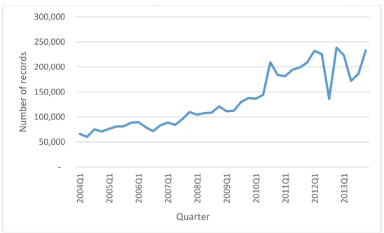
other hand, the increase of new drugs and people’s awareness of the importance of drug safety has caused rapid growth on the number of ADR’s reports to SRSs over the past few years. From 2004 to 2013, FAERS has collected over five millions of ADR records as shown in Figure 1.2. This further lengthens the time to build contingency cube for our iADRs system.
Figure 1.1 The architecture of iADRs [7].
OLAP Engine Mining Engine Contingency Cube Data preprocessing FAERS database iADRs Data warehouse User User User Cube based mining Web Server IIS & C#
3
Figure 1.2 The size of published FAERS data.
Recently, the MapReduce parallel computing framework proposed by Google [20] has achieved great success to process large data set or computation-intensive work, including the problem of OLAP data cube computation [40][41]. This motivates us to this research, developing MapReduce-based methods for computing the ADR contingency cube.
1.2 Contributions
The main contributions of this thesis are:
1. We propose a two-phase MapReduce-based framework to compute ADR contingency cube, with Phase 1 responsible for generating an intermediate cube used in Phase 2 to compute the required contingency cube.
2. We propose three MapReduce-based methods for computing the intermediate cube, including MRA-MJ, MRA-SJ, and MRA-SMJ. We also develop a
50,000 100,000 150,000 200,000 250,000 300,000 2 0 04 Q 1 2 0 05 Q 1 20 06Q 1 2 0 07 Q 1 2 0 08 Q 1 2 0 09 Q 1 2 0 10 Q 1 2 0 11 Q 1 2 0 12 Q 1 20 13Q 1 N u mb er o f reco rd s Quarter
4
based method to compute the resulting ADR contingency cube from intermediate cube.
3. We evaluate all proposed MapReduce-based methods from aspects including running time, memory usage, and I/O overhead.
1.3 Thesis Organization
The organization of this thesis is as follows.
In Chapter 2, we present the background knowledge related to this thesis. Section 2.1 introduces ADR signal and summarize common detection methods. Section 2.2 introduces OLAP, data cube, and contingency cube. Section 2.3 introduces Google’s GFS and MapReduce, and the well-known Hadoop.
In Chapter 3, we survey some related work about computing data cube including sequential, parallel, and MapReduce-based approaches.
In Chapter 4, we present our data preprocessing and state the problem of contingency cube computation in the first two sections. Section 4.3 presents our proposed two-phase framework and details the design of three MapReduce-based methods for Phase 1 and the method for Phase 2.
In Chapter 5, we describe the results on evaluating the two-phase approach, comparing our proposed three intermediate cube computation methods with the prevailing CubeGen [41] method and evaluating the performance of our method for Phase 2.
5
Background Knowledge
2.1 ADR Signal Detection
An ADR signal usually is represented as an association rule as follows, which is composed of drugs, reactions with possible predicate attributes. The predicate attribute is the patient’s physiological data, e.g., age, sex, weight.
[Predicate1, Predicate2, …], Drug → Reaction
One of the most famous ADRs is caused by Thalidomide. Many pregnant women took the drug to relieve their morning sickness but in 1960s experts discovered Thalidomide led to serious birth defects in more than ten thousands children. For this example, this ADR rule can be represented as follows.
Sex = female, Drug = Thalidomide → Reaction = Serious birth defects
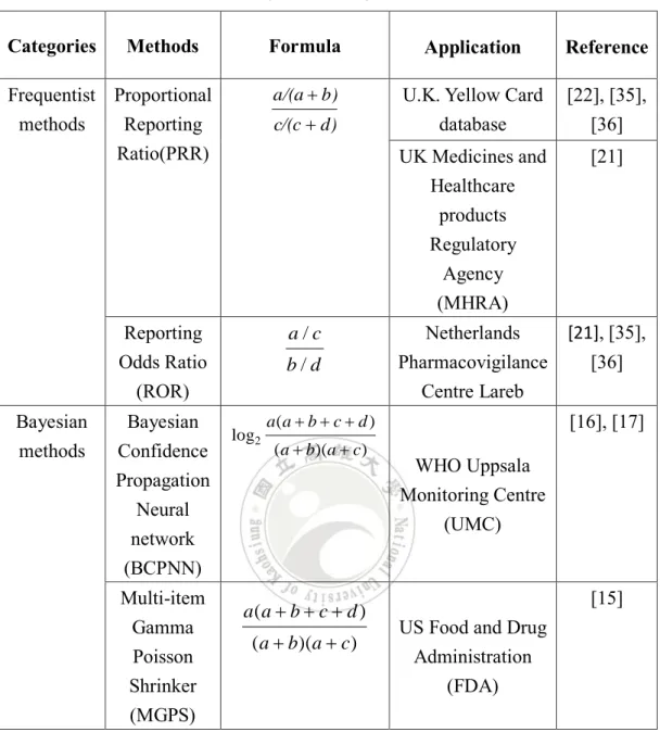
The purpose of ADR detection is to discover as earlier as possible suspected ADR signals from large amount of ADR reporting events. In the literature, the ADR signal detection methods can be divided into two categories: Frequentist methods and
Bayesian methods [18]. Because the ADR detection methods are beyond the scope of
6
Table 2.1 A summary of ADR signal detection methods.
Categories Methods Formula Application Reference
Frequentist methods Proportional Reporting Ratio(PRR) d) c/(c b) a/(a
U.K. Yellow Card
database [22], [35], [36] UK Medicines and Healthcare products Regulatory Agency (MHRA) [21] Reporting Odds Ratio (ROR) d b c a / / Netherlands Pharmacovigilance Centre Lareb [21], [35], [36] Bayesian methods Bayesian Confidence Propagation Neural network (BCPNN) WHO Uppsala Monitoring Centre (UMC) [16], [17] Multi-item Gamma Poisson Shrinker (MGPS)
US Food and Drug Administration
(FDA)
[15]
Both kinds of detection methods rely on the statistical 2*2 contingency table to calculate the strength of an ADR signal. Table 2.2 shows a typical 2*2 contingency table, where value a represents the number of reports in SRSs containing the drug and the reaction; value b means the number of reports containing the drug but not the reaction; value c means the number of reports containing the reaction but not the drug; and value d means the number of reports neither not containing the drug nor the reaction.
) )( ( ) ( log2 c a b a d c b a a ) )( ( ) ( c a b a d c b a a
7
Table 2.1 The 2*2 contingency table for ADR analysis. Suspected reaction Other reactions
Observed drug a b
Other drugs c d
2.2 OLAP, Data Cube, and Contingency Cube
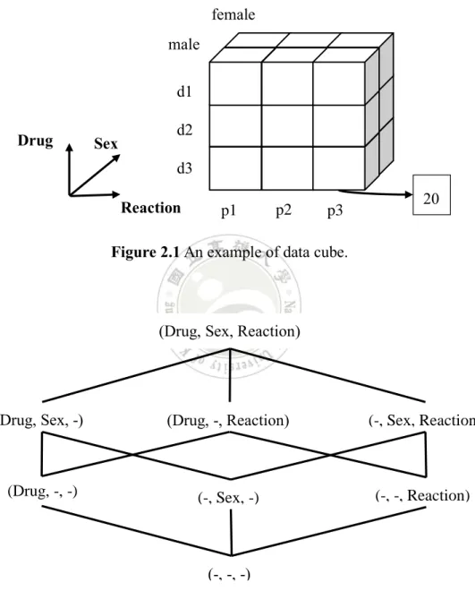
The concept of On-line Analytical Processing (OLAP) was first proposed by Codd [19], which is an analysis tool for front-end users of data warehouses. Through OLAP the analysts can perform multidimensional view of the accessed information. OLAP’s multidimensional data can be represented by different ways like data cube, cross table, and relation table; among them, data cube is the most adopted structure. For instance, Figure 2.1 depicts a three-dimensional data cube composed of Drug, Sex, and Reaction attributes. Each cell in the data cube stores a measured value interesting to the analysts, such as count, average, max, min. In this example, the cell value denotes count. When the analyst needs to know the count of some multi-item, e.g., {Sex male, Drug d3, Reaction p2}, the corresponding cell at the lower right corner provides an intermediate result, meaning that there are 20 records containing that multi-item in the data.
As OLAP aims at providing multidimensional analysis, the analysts may want to view the interested measure from all possible combinations of dimensions. To meet such a demand, the constructed data cube has to consist of all possible subcubes (or called cuboids) corresponding to all dimension combinations. In Figure 2.1, there are three different dimensions, so in total we have eight different cuboids, as shown in Figure 2.2. Besides, there exist aggregation dependencies between these cuboids. For example, the cuboid (Drug, Sex) can be computed from cuboid (Drug, Sex, Reaction)
8
by performing a simple accumulation along dimension Reaction. So we say (Drug, Sex) ≼ (Drug, Sex, Reaction), where “≼” denotes the dependency relation. This structure indeed is a lattice of cuboids.
Figure 2.1 An example of data cube.
Figure 2.2 An example cuboid lattice derived from dimensions Drug, Sex, and
Reaction. p3 Sex Drug Reaction male female d1 d2 d3 p2 20 p1
(Drug, Sex, Reaction)
(Drug, Sex, -) (Drug, -, Reaction) (-, Sex, Reaction)
(Drug, -, -) (-, Sex, -) (-, -, Reaction)
9
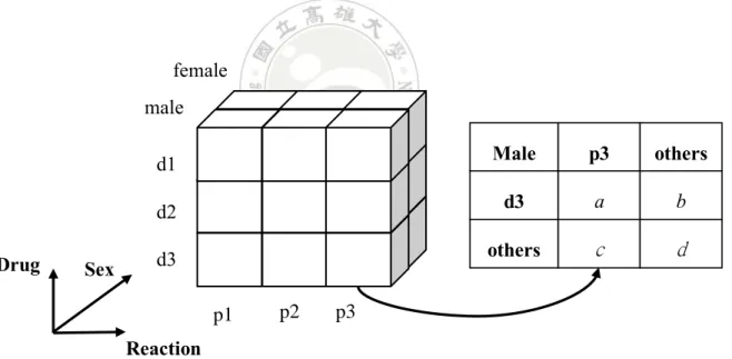
Contingency cube [30] is a new data cube structure used to accelerate ADR signal detection. Each cell in a contingency cube stores a contingency table as shown in Figure 2.3. In this way, when an ADR rule is required for analysis, the rule’s strength can be computed immediately by direct accessing the contingency table stored in the contingency cell. In Figure 2.3, the table can be used to compute the strength of the following ADR rule.
Sex Male, Drug d3 → Reaction = p3
Our iADRs system relies on the contingency cube to provide an interactive analysis platform, through which analysis can perform OLAP-like analysis and detection of ADR signals as soon as possible.
Figure 2.3 An illustration of contingency cube.
2.3 Cloud Computing and Hadoop
Cloud computing [8] refers to an internet-based platform that provides shared processing resources and data to realize ubiquitous computing services demanded by
p3 Sex Drug Reaction male female d1 d2 d3 p2 Male p3 others d3 others a c b d p1
10
end users. One of the main driving forces is Google, especially after in 2003 they sharing the design of their distributed system GFS [23] and parallel computing model MapReduce [20].
Google File System (GFS) [23] is a scalable distributed file system, which can be run on inexpensive commodity hardware yet exhibit good fault tolerance. Although Google says this system has successfully met their needs and it is widely deployed on their products, Google chose not open the source code of GFS.
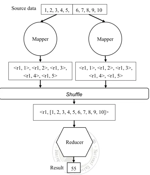
MapReduce [20] is a programming model used for processing large data sets. An example is shown in Figure 2.3 for summing numbers 1 to 10. First, each mapper is responsible for a partition of data, transforming the input number to intermediate <key, value> pair. In this example, all numbers are transformed to the same key, r1, with the number being assigned to the value. The shuffle function then sends those intermediate <key, value> pairs with the same key to the responsible reducer, wherein their values are appended to a value list. Finally, the reducer function executes some predefined aggregation function over the value list for each key. In this example the reducer has received only one key and value list. It then performs a simple summation of all numbers in the value list.
Hadoop, created by Doug Cutting [4], is an imitation of Google’s GFS and MapReduce. In January 2006, Hadoop was split from Nutch and more related projects were developed. Today, the term Hadoop is not just the base modules, but also refers to the ecosystem. The kernel modules to Hadoop are Hadoop Distributed File System (HDFS) and Hadoop MapReduce. Below we briefly describe HDFS and explain how HDFS and MapReduce work together.
11
Figure 2.4 An example of MapReduce for summing numbers.
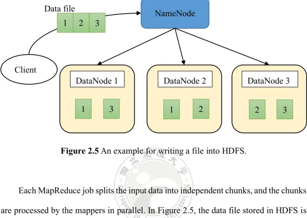
HDFS adopts the master and slave architecture. An HDFS cluster master, NameNode, is responsible for executing file system namespace like opening, closing, and renaming files. As shown in Figure 2.5, the client requests to save a file in HDFS. NameNode then splits the file into few blocks of fixed size, i.e., in this example is 3. The blocks will be replicated and saved into different slaves, i.e., DataNodes. This makes HDFS a highly fault-tolerant system. In this example, if DataNode 3 fails, its data can be quickly recovered from DataNodes 1 and 2. Another advantage of HDFS is efficiency. For instance, if we need to process block 2, HDFS provides interfaces for
1, 2, 3, 4, 5, Mapper Mapper 6, 7, 8, 9, 10 <r1, 1>, <r1, 2>, <r1, 3>, <r1, 4>, <r1, 5> <r1, 1>, <r1, 2>, <r1, 3>, <r1, 4>, <r1, 5> Shuffle <r1, [1, 2, 3, 4, 5, 6, 7, 8, 9, 10]> Reducer Source data 55 Result
12
moving the application to DataNode 2 or DataNode 3, rather than moving the block because “Moving computation is cheaper than moving data” [6].
Figure 2.5 An example for writing a file into HDFS.
Each MapReduce job splits the input data into independent chunks, and the chunks are processed by the mappers in parallel. In Figure 2.5, the data file stored in HDFS is split into three blocks, so the MapReduce job will invoke three mappers to handle this input source. Data file Client NameNode DataNode 1 DataNode 2 DataNode 3 1 3 1 2 2 3 1 2 3
13
Related Work
In this chapter, we describe related work on data cube computation, including sequential methods, parallel methods, and MapReduce-based methods.
3.1 Sequential Cube Computation
After Codd proposed the concept of OLAP, Jim Gray et al. [26] proposed the term
data cube and presented some optimization tips for data cube computation, like sorting
and hashing. The basic concept of sort- and hash-based methods is grouping data before the aggregation begins so as to reduce unnecessary data scanning. Figure 3.1 is an example of sort-based method, where the data is sorted by Drug, Sex, and Reaction. When the program wants to aggregate the measure of a specific drug, e.g., d0, it does not need to scan all data because all records containing ‘d0’ are nearby.
14
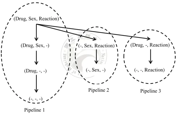
Since Gray et al.’s work, many more efficient methods have been proposed. Agarwal et al. [14] is one of early studies. They proposed two kinds of computing approaches, Pipesort and Pipehash, and also used Gray et al.’s sorting and hashing strategies. Figure 3.2 depicts a cube lattice that is split into three pipelines. For example, when cuboid (Drug, Sex, Reaction) is aggregated, that sorted data ordered by Drug, Sex, Reaction can be used immediately to aggregate the following cuboids (Drug, Sex, -), (Drug, -, -), and (-, -, -). Agarwal et al. named this concept share-sort.
Figure 3.2 An example of Agarwal et al’s pipesort method.
3.2 Parallel Cube Computation
Since earlier methods compute data cube sequentially, if the data set is of high dimension or is too large, the cube computation will spend a lot of time to complete. This motivates the development of parallel cube computing methods. Goil and
(Drug, Sex, Reaction)
(Drug, Sex, -) (Drug, -, Reaction)
(Drug, -, -) (-, -, Reaction) (-, -, -) (-, Sex, Reaction) (-, Sex, -) Pipeline 1 Pipeline 2 Pipeline 3
15
Choudhary [24], [25] first modified Agarwal et al.’s method to compute data cube in parallel, but their method assumed that all data can be stored in memory, so is not suitable for large data set. During the same period, Lu et al. [31] proposed a parallel method for computing ROLAP cube, which is based on hashing method, though their method is a brute force approach. Later Muto and Kitsuregawa [32] proposed another method with better load-balancing, but they provided no implementation and no experimental result.
3.3 MapReduce-based Cube Computation
Inspired by recent success of MapReduce computing framework on processing large data set or computation-intensive work, some researchers have used MapReduce framework to build OLAP data cube, including Sergey and Yurk [37], You et al. [42], Nandi et al. [33], [34], and Lee et al. [29]. One of the prevailing methods is the CubeGen method proposed by Wang et al. [41].
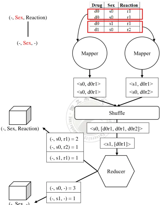
Method CubeGen splits the cube lattice is a way similar to Agarwal et al.’s method and assigns a MapReduce job to handle each pipeline batch. The Mapper function chooses a dimension that exists in all cuboids to be computed in the pipeline and assign that dimension as the output’s key, along with other dimensional values as the output value. Then the shuffle function sends all outputs with the same key to the corresponding reducer. Each reducer is responsible for generating the final aggregation for each cuboid of the assigned pipeline batch. As shown in Figure 3.3, for each key value, e.g., s0, the reducer overlooks one dimensional value, e.g., d0, and group by all values in the value-list to achieve the aggregated count. In this example, it yields (-, s0,
16
r1) = 2 and (-, s0, r2) = 1. The process continues to overlook more dimensional values to obtain aggregation results for other cuboids.
Figure 3.3 An example of CubeGen for computing the pipeline batch consisting of (-,
See, Reaction) and (-, Sex, -). (-, Sex, Reaction) (-, Sex, -) Mapper Mapper <s0, d0r1> <s0, d0r1> <s1, d0r1> <s0, d0r2> Reducer Shuffle <s0, [d0r1, d0r1, d0r2]> <s1, [d0r1]> (-, Sex, Reaction) (-, Sex, -) (-, s1, r1) = 1 (-, s0, r1) = 2 (-, s0, r2) = 1 (-, s1, -) = 1 (-, s0, -) = 3
17
The Proposed MapReduce-based
Contingency Cube Computation
In this chapter, we present our proposed MapReduce-based methods for computing the ADR contingency cube. We use the open data of U.S. FDA Adverse Event Reporting System (FAERS) as the data source. This data, unfortunately, is not clean, which has many uncertainties. So Section 4.1 will explain how we process the data before building contingency cube.
4.1 Data Preprocessing
The main problems of FAERS data are duplicate reporting and non-standardized drug names. The former refers to the existence of duplicate records that correspond to the same ADR event due to different reporting sources and follow-up review of the event.The latter means that the drug names are not standardized; different names may refer to the same drug. The reason is very complicated, so the detailed process for normalizing drug name is beyond the scope of this thesis. We only present a brief description. The interested readers can refer to [27] for the details.
The FAERS database always releases new reports quarterly. Each time as new quarter data is reported, the preprocessing workflow shown in Figure 4.1 is executed to generate the prepared data. In the following, we describe each of these steps.
18
Figure 4.1 The preprocessing workflow for generating the prepared data.
1. Data selection: Besides, the whole FAERS data consists of seven tables, as
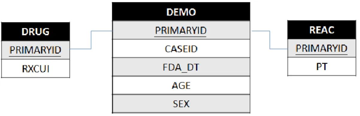
shown in Figure 4.2, but only some attributes, including Sex, Age, Drug, and PT (preferred term for symptom), are essential for ADR analysis. Figure 4.3 shows the essential part of schema of the FAERS dataset.
FAERS 1. Data Selection
2. Deduplication
3. Drug name standardization
4. Transformation
19
Figure 4.2 The FAERS ADR data schema.
20
2. Deduplication: In the FAERS system, each patient’s ADR event has a unique
code, namely CASEID. Since the same case may be reported many times, each reporting record is identified by a unique PRIMARYID. For the group of records that have the same CASEID, we only have to leave one record. We choose that one with the latest FDA_DT (the date reporting to FDA).
3. Drug name standardization: For some reasons, a drug may have many
different names, so we need to normalize drug name before counting record. The US NLM is the biggest medicine library in the world. We use their RxNorm [9] which is a normalized naming service to transform DRUGNAME attribute into unique identifier, RXCUI.
4. Transformation: This step performs some attribute transformation and stores
the output data prepared for cube computation. First, we discretize the original numerical Age attribute into ten categorical ranges as shown in Table 4.1. Next, FAERS database is relational, so all the Drugs and PTs of a single event have to be normalized into different records, stored in different tables. Direct aggregation from such data many cause duplicate counting of event occurrence. So we join the records into a single record.
The prepared data is stored as a text file. There are four attributes, including AGE, SEX, DRUG, and PT, delimitated by pound sign (#). Multiple values of DRUG and PT attributes are delimitated by dollar sign ($). Figure 4.4 is a simple example. This format also can compress data for our MapReduce-based computation. As shown in Table 4.2, this format saves about 90 percent of size and number of records.
21
Table 4.1 Discretization of the AGE attribute.
Tag Range Meaning
0 0 Source value is missing or problematic, e.g.,
not a numerical or large than 116 years.
1 0 Infant, Newborn
2 1 to 23 months Infant
3 2 to 5 years Child Preschool
4 6 to 12 years Child
5 13 to 18 years Adolescent
6 19 to 24 years Young Adult
7 25 to 44 years Adult
8 45 to 64 years Middle Aged
9 65 to 79 years Aged
10 over 80 years Aged+
Attributes
Data file AGE SEX DRUG PT
Cleaned data a1 s1 d1, d2 p1, p2
Source data for
MapReduce a1#s1#d$d2#p1$p2
22
Table 4.2 Number of records before and after packing.
Size Number of records
Unpacked 1.3 GB 49,540,834
Packed 150 MB 3814,472
4.2 Problem of ADR Contingency Cube
Computation
The iADRs system provides OLAP-like ADR signal detection and analysis via multiple dimensions, i.e., Age and Sex attributes. Since attributes Drug and PT are mandatory for ADR signal, the contingency cube consists of four kinds of cuboids, as shown in Figure 4.4. In this paper, a contingency cuboid is denoted by C(P1, P2, Drug,
PT) and the missing predicate attribute is denoted by minus symbol ‘-‘. For instance, C(Age, -, Drug, PT) represents the contingency cube with predicate Age.
Figure 4.4 Four kinds of cuboids in the ADR contingency cube.
Each cell in a cuboid stores the counting statistics of contingency table. For example, Figure 4.5 shows the corresponding contingency cell from C (-, SEX, DRUG, PT) for answering query {SEX = Male, DRUG = d3 and PT = p3}.
C(Age, -, Drug, PT) C(-, Sex, Drug, PT) C(-, -, Drug, PT) C(Age, Sex, Drug, PT)
23
Figure 4.5 An example of contingency cell in cuboid (-, SEX, DRUG, PT).
The problem of ADR contingency cube computation is: Given the SRS dataset (FAERS data) that has been prepared according to the preprocessing framework presented in Section 4.1, we want to generate all the contingency cuboids forming the contingency cube.
4.3 Basic Concept
In this section, we present the basic concept of computing contingence cubes by MapReduce framework. Intuitively, the values of each cell in a contingency cuboid can be obtained by aggregating the occurrence along the source data. However, the computation of b, c, d values in each contingency cell involves negative item, which is not directly accessible from the data and so hard to fit to the (key, value) structure required by MapReduce framework. The solution is to avoid counting the negative item directly. Instead, we can compute the occurrence of negative items through that of positive items [30]. In general, for a contingency table composed of predicate, P1 = v1,
P2 = v2, …, Pk = vk, Drug = dg, and PT = sm, Table 4.3 shows the formula for computing
C (-, SEX, DRUG, PT) p3 p1 M F p2 d1 d2 d3 Male p3 others d3 others 10 50 90 150 *
24
cell a, b, c, d values, where count (v1, v2, …, vk, dg, sm) denote the occurrences of
itemset {v1, v2, …, vk, dg, sm}.
Table 4.3 The formula for the computation of each cell
in a 2×2 contingency table [30].
Cell value The formula
a count(v1, v2, …vk, dg, sm)
b count(v1, v2, …vk, dg) - a
c count(v1, v2, …vk, sm) - b
d count(v1, v2, …vk) - a - b - c
Therefore, we use a two-phases approach to compute the contingency cube. First, we compute the occurrences of positive itemsets, i.e., count (v1, v2, …, vk, dg, sm), count
(v1, v2, …, vk, dg), count (v1, v2, …, vk, sm), and count (v1, v2, …, vk), then from which
we can compute the values of b, c, d.This two-phases approach framework is shown in Figure 4.6, where intermediate cubes are used to store the occurrences of positives itemsets.
Figure 4.6 The framework of two-phases MapReduce-based contingency cube
computation. Contingency Cube Source Data Phase 1 MRA-MJ MRA-SJ MRA-SMJ Intermediate cube Phase 2
25
We develop three different methods, MRA-MJ (MapReduce-based Aggregation via Multiple Jobs), MRA-SJ (MapReduce-based Aggregation via Single Job), and MRA-SMJ (MapReduce-based Aggregation via Smallest Multiple Jobs), for realizing Phase 1 to compute the intermediate cubes, which will be detailed in the following subsections.
26
4.4 Phase 1: Intermediate Cube Generation
The purpose of this phase is to create 16 intermediate cuboids (see Table 4.4) that are used for later computation of the contingency cube. Similar to the notation for contingency cube, we use I(A1, A2, A3, A4) to denote an intermediate cuboid aggregated by attributes A1, A2, A3, A4, and for simplicity, abbreviation is used for attribute name. For example, I(A, S, -, -) denotes the intermediate cube aggregated by Age and Sex. Figure 4.7 shows an example of the input and output for Phase 1, where each output record includes attribute values and count, delimitated by tab (\t).
Table 4.4 The 16 intermediate cuboids.
I(A, S, D, P) I(A, -, D, P) I(-, S, D, P) I(-, -, D, P) I(A, S, D, -) I(A, -, D, -) I(-, S, D, -) I(-, -, D, -) I(A, S, -, P) I(A, -, -, P) I(-, S, -, P) I(-, -, -, P) I(A, S, -, -) I(A, -, -, -) I(-, S, -, -) I(-, -, -, -)
Figure 4.7 An example of input and output for generating I(A, S, -, -) in Phase 1.
a1#s1#d1#p1 a1#s1#d2#p2 a1#s0#d1#p1 a2#s2#d2#p3 a2#s2#d3#p3 Source data Phase 1 a1#s1## 2 a1#s0## 1 a2#s2## 2
Aggregated by AGE & SEX
27
4.4.1 Method MRA-MJ
The concept of MRA-MJ is simple. As shown in Figures 4.8 each intermediate cuboid is computed by a MapReduce job, so there are 16 different MapReduce jobs. Each MapReduce job is activated by a group-by information sent from the client program. For example, the group-by information (Age, Sex) is send to the MapReduce job responsible for creating I(A, S, -, -) as shown in Figure 4.9. This group-by information also instructs the mapper which attributes are used as key, e.g., Age and Sex in this example.
Figure 4.8 An illustration of framework of MRA-MJ
Source data Client MapReduce job I(A, S, D, -) I(A, S, D, P) I(-, -, -, P) MRA-MJ
{Age, Sex, Drug, PT}
{Age, Sex, Drug} {PT}
28
Figure 4.9 An example workflow of MapReduce job
for computing I(A, S, -, -).
Source data a1#s1#d1#p1 a1#s1#d2#p2 a1#s0#d1#p1 a2#s2#d2#p3 a2#s2#d3#p3 Mapper {Age, Sex} Mapper {Age, Sex} Mapper {Age, Sex} Reducer Shuffle <”a2#s2##”, 1> <”a1#s0##”, 1> <”a2#s2##”, 1> <”a1#s1##”, 1> <”a1#s1##”, 1>
<”a2#s2##”, [1, 1]> <”a1#s0##”, [1]> <”a1#s1##”, [1, 1]>
Reducer Reducer
I(A, S, -, -)
29
The main disadvantage of MRA-MJ is I/O overhead. Because each MapReduce job needs to read the source data, the whole process requires sixteen times of data reading. So we design the second method MRA-SJ.
4.4.2 Method MRA-SJ
The MRA-SJ method invokes only one MapReduce job to generate all 16 cuboids. An illustration of the idea is shown in Figure 4.10.
Figure 4.10 An illustration of method MRA-SJ.
Source data Client
I(A, S, D, -) I(A, S, D, P)
MRA-SJ
{Age, Sex, Drug, PT} {Age, Sex, Drug, -}
… {-, -, -, PT}
MapReduce job {group-by attributes}
30
Each mapper is responsible for a partition of the input file. Once reading an input record, the mapper generates 16 output (key, value) combinations, corresponding to 16 different combinations (group-by) required by the 16 intermediate cuboids. The embedded shuffle function provided by the system then redirects all records of the same key into the same reducer task, wherein aggregation is performed to obtain the accumulated value (count). An example of this workflow is demonstrated in Figure 4.11.
The MRA-SJ method needs only one scan of the input file, thus can reduce lots of I/O overhead. However, each mapper works heavily to enumerate all key combinations, which is not executed in parallel.
In summary, this method wipes heavy I/O overhead by providing limited data parallelism and overlooking inherent computation parallelism for each partition. We thus propose the third method MRA-SMJ, endeavoring to exploit more computation parallelism without incurring too much I/O overhead.
31
Figure 4.11 An Example of MRA-SJ.
{Age, Sex, Drug, PT} {Age, Sex, Drug, -} …
{-, -, -, PT)
Source data a1#s1#d1#p1 a1#s1#d2#p2 a1#s0#d1#p1 a2#s2#d2#p3 a2#s2#d3#p3 {Age, Sex, Drug, PT}
{Age, Sex, Drug, -) … {-, -, -, PT} Mapper Mapper Shuffle <”a2#s2#d2#p3”, 1> <”a2#s2#d2#”, 1> … <”a2#s2#d3#p3”, 1> … <” a1#s1#d1#p1”, 1> <” a1#s1#d1#”, 1> … <” a1#s1#d2#p2”, 1> … I(A, S, -, -) Reducer
<”a2#s2##”, [1, 1]> <”a1#s0##”, [1]> <”a1#s1##”, [1, 1]>
Reducer Reducer
32
4.4.3 Method MRA-SMJ
Figures 4.12 is an illustration of MRA-SMJ, which hybridizes the advantages of MRA-MJ and MRA-SJ. Method MRA-SMJ generates all intermediate cuboids in a level-wise style, starting from the cuboid with the most number of dimensions downward to the one with no dimensions. Besides, MRA-SMJ adopts the smallest-parent strategy used in sequential computation of OLAP data cube [26]. That is, each MapReduce job chooses the parent cuboid with the smallest size as its input data. So this method also consists of multiple MapReduce jobs to finish the whole computation, meaning this method exploits more parallelism. For instance, I(A, S, -, -) is used by a MapReduce job to compute I(A, -, -, -) and I(-, S, -, -).
As Figure 4.12 illustrates, the MRA-SMJ method requires the size information of each cuboid to prepare the execution plan. Fortunately, the size of each cuboid is easily estimated, which is proportional to the number of distinct attribute value combinations. For example, there are 11 distinct values in Age and 3 in Sex, so the size of I(A, S, -, -) will approximately be 11 * 3 = 33.
33
Figure 4.12 An example workflow of MRA-SMJ
Source data I(A, S, D, P)
I(A, S, D, -) I(A, S, -, P) I(A, -, D, P) I(-, S, D, P)
I(A, S, -, -) I(A, -, D, -) I(-, S, D, -) I(A, -, -, P) I(-, S, -, P) I(-, -, D, P)
I(A, -, -, -) I(-, S, -, -) I(-, -, D, -) I(-, -, -, P)
34
4.5 Phase 2: Contingency Cube Computation
In this section, we present the method for Phase 2, computing the ADR contingency cube from the intermediate cube generated in Phase 1.
Since the ADR contingency cube is composed of four cuboids, C(Age, Sex, Drug, PT), C(-, Sex, Drug, PT), C(Age, -, Drug, PT), and C(-, -, Drug, PT), the intermediate cuboids can be classified to four groups, each of which contains cuboids with the same choice of predicate attributes, i.e., Age and Sex. For example, for contingency cuboid
C(Age, -, Drug, PT) we needs intermediate cuboid I(Age, -, Drug, PT), I(Age, -, Drug,
-), I(Age, -, -, PT), and I(Age, -, -, -). Figure 4.13 shows the grouping relationship between contingency cuboids and intermediate cuboids.
Figure 4.13 The relationship between intermediate cuboids
and ADR contingency cuboids.
The program for Phase 2 invokes four MapReduce jobs, each responsible for computing one of the four contingency cuboids. Here we present the workflow for computing C(Age, Sex, Drug, PT). See Figure 4.14.
C(Age, Sex, Drug, PT) C(-, Sex, Drug, PT)
C(-, -, Drug, PT) C(Age, -, Drug, PT) (A, S, D, P) (A, S, D, -) (A, S, -, P) (A, S, -, -) (A, -, D, P) (A, -, D, -) (A, -, -, P) (A, -, -, -) (-, S, D, P) (-, S, D, -) (-, S, -, P) (-, S, -, -) (-, -, D, P) (-, -, D, -) (-, -, -, P) (-, -, -, -)
35
Each mapper is responsible for transform the assigned input records, each into a (key, value) pair, with values of predicate attributes, i.e., Age and Sex, being the key, and others data like values of Drug, PT, and number of count being the value. Then the shuffle function redirects all output of mappers to reducers, with records of the same
key to the same reducer, wherein the resulting contingency cuboid C(Age, Sex, Drug,
PT) is computed.
Figure 4.15 shows the process of reducer for C(Age, Sex, Drug, PT). For each key, the reducer looks for each ‘drug#PT#count’ value, and the corresponding ‘drug##count’, ‘#PT#count’, ‘##count’ values to generate the contingency values a, b,
c, d. For example, as shown in Figure 4.15, value a of ADR rule (a1, s1, d1, p1) is 10;
value b is count of (Drug = d1), 50, minus value a, leading to 40; value c is count of (PT = p1) minus a, obtaining 50; and d equals to the total count (200) minus a, b, c, obtaining 100.
36
Figure 4.14 An example of Phase 2’s MapReduce job.
< “a1#s1#d1#p1”, 10 > < “a2#s2#d2#p2”, 20> I(A, S, D, P) Mapper < “a1#s1#d1#”, 50 > < “a2#s2#d2#”, 60 > I(A, S, D, -) < “a1#s1##p1”, 60 > < “a2#s2##p2”, 70 > I(A, S, -, P) < “a1#s1##”, 200 > < “a2#s2##”, 300 > I(A, S, D, -) < “a1#s1”, [ “d1#p1#10”, “d1##50”, “#p1#60”, “##200”] > Reducer
C(Age, Sex, Drug, PT)
Mapper Mapper Mapper
< “a1#s1”, “d1#p1#10” > < “a2#s2”, “d2#p2#20> < “a1#s1”, “d1##50” > < “a2#s2”, “#d2##60” > < “a1#s1”, “##p1#60” > < “a2#s2”, “##p2#70” > < “a1#s1”, “###200” > < “a2#s2”, “###300” > Shuffle < “a2#s2”, [ “d1#p1#20”, “d1##60”, “#p1#70”, “##300”] > Reducer <“a2#s2#d1#p1”, “20#40#50#190”> <“a1#s1#d1#p1”, “10#40#50#100”>
37
Figure 4.15 An example of reducer for computing C(Age, Sex, Drug, PT).
< “a1#s1”, [“d1#p1#10”, “d1##50”, “#p1#60”, “##200” , “d2#p2#50”, “d2##70”, “#p2#90”] > d1#p1, 10 d2#p2, 50 Value a d1, 50 d2, 70 DRUG p1, 60 p2, 90 PT 200 Total 10 40
C(Age, Sex, Drug, PT)
38
Empirical Study
5.1 Environment
and Experimental Design
We conducted a series of experiments to evaluate the performance of our proposed two-phase framework for computing ADR contingency cube. All experiments were tested using the FAERS datasets from 2004Q1 to 2013Q4. Statistics of these datasets are shown in Table 5.1.
Table 5.1 Statistics of FAERS datasets.
We established a Hadoop cluster composed of three nodes installed with Cloudera distribution. Each node has independent HDD and linked with 1Gbps networks. All nodes were running CentOS 6 and JAVA 8 environment. A summary of the specification is shown in Table 5.2. All programs were opened on Github [12].
Dataset Record # Size (MB) Drug # PT #
2004 201205 9 2420 9121 2005 222805 10 2446 9667 2006 235954 11 2455 9881 2007 258200 11 2423 9871 2008 298109 12 2475 10256 2009 321292 14 2564 10626 2010 461027 19 2636 11098 2011 523946 22 2679 11592 2012 610359 26 2798 12138 2013 681571 28 2875 12384 Total 3814468 162 25771 106634
39
Table 5.2 Specification of the Hadoop cluster used in our experiment.
Node CPU RAM HDD
1 Intel i7-4790 32 GB WD blue 2TB
2 Intel Q6600 8 GB WD blue 1TB
3 Intel Q8300 4 GB WD blue 1TB
We inspected the performance of our proposed frameworks, including Phase 1 and 2, from the viewpoints of execution time, I/O overhead, and memory usage.
5.2 Evaluation of Phase 1
We first compared our proposed three methods for Phase 1. Since the intermediate cube indeed equals to the OLAP data cube, we also considered a prevailing MapReduce-based method for OLAP cube computation, CubeGen [41]. Among the four methods, MRA-MJ, MRA-SMJ, and CubeGen invoke multiple MapReduce jobs to finish the work. The number of jobs needed by each method is reported in Table 5.3.
Table 5.3 Number of jobs required by each method. Method’s Name Number of jobs Maximum parallel jobs
MRA-MJ 16 16
MRA-SJ 1 1
MRA-SMJ 9 3
CubeGen 6 6
We first examined the execution time of four methods. As shown in Figure 5.1, MRA-SMJ is the fastest to complete the computation of intermediate cube in our environment. Method MRA-MJ though exploits the most number of jobs performs the worst on running time, because it incurs the largest amount of I/O readings. As shown
40
in Figure 5.2, the I/O overhead consumed by MRA-MJ is 16 times of that by MRA-SJ, 1.6 times of MRA-SMJ, and 2.5 times of CubeGen. Method MRA-SJ spends the smallest I/O reading because it reads source data once.
Figure 5.1 Comparison on execution time.
Method CubeGen, though consumes less I/O overhead than MRA-SMJ, executes longer than MRA-SMJ.After checking the log of execution, we found CubeGen spend too much time on mapper task. This is because attributes Drug and PT of the source data contain multiple values, so each mapper needs to scan these two multi-valued attributes to enumerate all Drug and PT pairs. On the other hand, our method MRA-SMJ read source data once as input to the first job to create C(A, S, D, P), but all MapReduce jobs of CubeGen use source data as the input.
200 400 600 800 1,000 1,200 1,400 1,600
MRA-MJ MRA-SJ MRA-SMJ CubeGen
Ru n ti me(s ec. )
41
Figure 5.2 Comparison on amount of I/O reading from HDFS.
We then examined the amount of memory usage. Figure 5.3 depicts the total amount of memory usage for each method. Not surprisingly, all methods consumed more memory to execute mapper than to run reducer. In our experiments, each MapReduce job invokes one reducer, while the number of mappers is decided by Hadoop system and each input’s block is assigned to one mapper task. Since our source data were split into five blocks stored in HDFS, there were five mappers executed to complete this job.
Method MRA-MJ uses the largest amount of memory because it invokes 16 jobs, and MRA-SJ requires the least amount. At first glance, it seems that MRA-MJ requires larger memory resource. This however does not reflect the real situation. Figure 5.4 depicts the timeline memory usage of MRA-MJ and MRA-SMJ. Method MRA-SMJ consumes more peek amount of memory than that by MJ, which means MRA-SMJ has a higher demand on memory resource. CubGen requires similar peek amount of memory to MRA-MJ. MRA-SJ consumes the smallest amount due to it invoking only one MapReduce.
500 1,000 1,500 2,000 2,500 3,000
MRA-MJ MRA-SJ MRA-SMJ CubeGen
42
Figure 5.3 Comparison on memory usage.
Figure 5.4 Comparison on timeline memory usage.
In summary, method MRA-SMJ, in our cluster environment, is the fastest among these methods, followed by MRA-SJ, CubeGen, and MRA-MJ. However, our cluster consists only three nodes, which maybe awkward to fulfill all exploitable parallelism
50,000 100,000 150,000 200,000 250,000 300,000
MRA-MJ MRA-SJ MRA-SMJ CubeGen
MB 20,000 40,000 60,000 80,000 100,000 120,000 140,000 1 2 3 4 5 6 7 8 9 1 0 1 1 1 2 1 3 1 4 1 5 1 6 1 7 1 8 1 9 2 0 2 1 2 2 2 3 2 4 2 5 MB Time (min.)
43
provided by each method. If the cluster has enough nodes to work, we argue that method MRA-MJ is a better choice because it exploits more parallel jobs simultaneously.
The total size of the intermediate cube is approximately 2.5 GB; detailed statistics of each cuboid is shown in Table 5.4.
Table 5.4 Statistics of intermediate cuboids. Intermediate cuboid Size (KB) Record #
I(-, -, -, -) 2 123 I(A, -, -, -) 19 1,324 I(-, S, -. -) 6 364 I(-, -, D, -) 3,158 192,488 I(-, -, -, P) 9,810 640,862 I(A, S, -, -) 59 3,956 I(A, -, D, -) 12,633 737,293 I(A, -, -, P) 29,366 1,812,263 I(-, S, D, -) 6,652 386,542 I(-, S, -, P) 17,654 1,089,515 I(-, -, D, P) 454,629 23,169,394 I(A, S, D, -) 21,632 1,199,006 I(A, S, -, P) 44,852 2,615,619 I(A, -, D, P) 665,365 32,200,940 I(-, S, D, P) 570,253 27,683,207 I(A, S, D, P) 773,146 35,708,435
5.3 Evaluation of Phase 2
We then inspected the performance of Phase 2. Table 5.5 shows statistics of the four contingency cuboids. The total size of the contingency cube is 3.6 GB, which is 24 times of the source data.
Figure 5.5 depicts the execution time (Phase 2) to generate each contingency cuboid, where the execution time for each method used in Phase 1 is shown for
44
comparison. Phase 2 needs about 12 minutes to compute the whole contingency cube from intermediate cube. If we choose MRA-SMJ in Phase 1, our framework can compute the contingency cube within half an hour. Before using the MapReduce platform, our iADRs system computed contingency cube on a single machine running Microsoft Windows 7 and SQL Server 2008. The programs were coded in C# invoking SQL, which required about one and half month to compute the ADR contingency cube. Compared with this old approach, our MapReduce-based approach exhibits around 2,160 speedups!
Table 5.5 Statistics of the ARD contingency cube. Contingency cuboid Size (MB) Record #
C(-, -, D, P) 993 23,169,394
C(A, -, D, P) 1,110 32,200,940
C(-, S, D, P) 731 27,683,207
C(A, S, D, P) 878 35,708,435
Figure 5.5 Running time of Phase1 and Phase 2.
0 5 10 15 20 25 30 35 40
MRA-MJ MRA-SJ MRA-SMJ CubeGen
45
We also examined the I/O overhead (Figure 5.6) and memory usage (Figure 5.7) for Phase 2. The results demonstrate that Phase 2 consumes approximate the same I/O overhead as method MRA-MJ because Phase 2 needs to read many intermediate cuboids. Compared with Phase 1, the computation executed in Phase 2 is much more complicated than that in Phase 1, so it demands more memory than Phase 1.
Figure 5.6 Amount of I/O reading from HDFS for Phase 1 and Phase 2.
Figure 5.7 Memory usage of Phase 1 and Phase 2.
1,000 2,000 3,000 4,000 5,000 6,000
MRA-MJ MRA-SJ MRA-SMJ CubeGen
MB Phase 1 Phase 2 100,000 200,000 300,000 400,000 500,000 600,000 700,000 800,000 900,000
MRA-MJ MRA-SJ MRA-SMJ CubeGen
MB
46
Conclusions and Future Work
6.1 Conclusions
Detecting suspicious ADR signals from SRSs has been an important problem in pharmacovigilance. Our established ADR detection and analysis system, iADRs, can provide an interactive platform for analysts. But the contingency cube used by iADRs requires lots of computations to construct.
In this thesis we have proposed a two-phase MapReduce-based framework to compute the ADR contingency cube. In Phase 1, we have proposed three MapReduce-based methods to aggregate and compute intermediate cube. In Phase 2, we have presented a MapReduce-based method to compute contingency cube from intermediate cube.
We have used FAERS database to evaluate all proposed MapReduce-based methods and provided advises for choosing suitable approach considering running time, memory usage, and I/O overhead. Compared with the current approach of iADRs, this MapReduce-based workflow only needs half an hour to compute the contingency cube. Because our framework is built on Hadoop system, its performance is easy to magnify by adding more computing resources. This also inspires us to incorporate other SRS data, like the Canada Vigilance Adverse Reaction Online Database [3] into our system.
47
6.2 Future Work
Although our framework can quickly compute the contingency cube, it needs to rebuild the whole cube to incorporate new data released by FAERS. A better way is to update part of the contingency cube to reflect the source evolution. But the contingency cube is more complicated than OLAP cube, because each cell stores a contingency table and the values of b, c, and d are dependent on the content of other cells. So our first challenging is to develop a new approach to incrementally update the ADR contingency cube efficiently.
Another interesting issue is to find more efficient computing framework. In MapReduce, each intermediate (key, value) pair always has to be written back to disk before sends to the reducers, which incurs lots of I/O overhead and so easy to become the performance bottleneck. Nowadays, more and more computing frameworks have been proposed, like Spark [2] and Flink [1]. They can cache intermediate data in memory for next computing stage, so are more efficient than MapReduce. Furthermore, these frameworks can also be run on Hadoop, which means they have many supports from open source community. Recently, more related applications have been developed on Spark and Flink. Our next step is to redesign our method for contingency cube computation on these new computing frameworks.
48
References
[1] Apache Flink, Available: https://flink.apache.org/, [July 22, 2016]. [2] Apache Spark, Available: http://spark.apache.org/, [July 22, 2016].
[3] Canada Vigilance Adverse Reaction Online Database, Available:
http://www.hc-sc.gc.ca/dhp-mps/medeff/databasdon/index-eng.php, [July 21, 2016].
[4] D. Cutting, Available: https://issues.apache.org/jira/browse/INFRA-700, [July 20, 2016].
[5] FDA's Adverse Event Reporting System (FAERS), Available:
http://www.fda.gov/Drugs/GuidanceComplianceRegulatoryInformation/Surveilla nce/AdverseDrugEffects/default.htm, [July 21, 2016].
[6] HDFS Architecture, Available:
https://hadoop.apache.org/docs/r2.7.2/hadoop-project-dist/hadoop-hdfs/HdfsDesign.html, [July 19, 2016]. [7] iADRs, Available: http://iadr.csie.nuk.edu.tw, [July 21, 2016].
[8] P. Mell and T. Grance, The NIST Definition of Cloud Computing, Available:
http://nvlpubs.nist.gov/nistpubs/Legacy/SP/nistspecialpublication800-145.pdf, [July 20, 2016].
[9] National Library of Medicine RxNorm, Available:
https://www.nlm.nih.gov/research/umls/rxnorm/, [July 7, 2016].
[10] Taiwan National Adverse Drug Reactions Reporting System, Available:
https://adr.fda.gov.tw/Manager/WebLogin.aspx, [July 21, 2016].
[11] Uppsala Monitoring Centre (UMC), Available: http://www.who-umc.org, [July 21, 2016].
[12] M.S. Wang, MRiADRs, Available: https://github.com/Phate334/MRiADRs, [July 7, 2016].
49
[13] Yellow Card Scheme, Available: https://yellowcard.mhra.gov.uk, [July 21, 2016]. [14] S. Agarwal, R. Agrawal, P.M. Deshpande, A. Gupta, J.F. Naughton, R. Ramakrishnan, and S. Sarawagi, “On the computation of multidimensional aggregates,” in Proceedings of 22th International Conference on Very Large Data
Bases, 1996, pp. 506-521.
[15] J.S. Almenoff, K.K. LaCroix, N.A. Yuen, D. Fram, and W. DuMouchel, “Comparative performance of two quantitative safety signaling methods: implications for use in a pharmacovigilance department,” Journal of Drug Safety, vol. 29, no. 10, pp. 875-887, 2006.
[16] A. Bate, “Bayesian confidence propagation neural network,” Journal of Drug
Safety, vol. 30, no. 7, pp. 623-625, 2007.
[17] A. Bate et al, “A Bayesian neural network method for adverse drug reaction signal generation,” European journal of clinical pharmacology, vol. 54, no. 4, pp. 315-321, 1998.
[18] B.K. Chen and Y.T. Yang, “Post-marketing surveillance of prescription drug safety: past, present, and future,” Journal of Legal Medicine, vol. 34, no. 2, pp. 193-213, 2013.
[19] E.F. Codd, S.B. Codd, and C.T. Salley, Providing OLAP (On-Line Analytical
Processing) to User-Analysts: An IT Mandate, E. F. Codd & Associates, 1993.
[20] J. Dean, and S. Ghemawat, "MapReduce: simplified data processing on large clusters,” Communications of the ACM, vol. 51, no. 1, pp. 107-113, 2008.
[21] G. Deshpande, V. Gogolak, and S.W. Smith, “Data mining in drug safety,”
50
[22] S.J. Evans, P.C. Waller, and S. Davis, “Use of proportional reporting ratios (PRRs) for signal generation from spontaneous adverse drug reaction reports,” Journal of
Drug Safety, vol. 10, no. 6, pp. 483-486, 2001.
[23] S. Ghemawat, H. Gobioff, and S.-T. Leung, "The Google files system," in
Proceedings of 19th ACM Symposium on Operating Systems Principles, 2003, pp.
29-43.
[24] S. Goil and A.N. Choudhary, “High performance OLAP and data mining on parallel computers,” Data Mining and Knowledge Discovery, vol. 1, no. 4, pp. 391-417, 1997.
[25] S. Goil and A.N. Choudhary, “A parallel scalable infrastructure for OLAP and data mining,” in Proceedings of International Symposium on Database
Engineering and Applications, 1999, pp. 178-186.
[26] J. Gray, S. Chaudhuri, A. Bosworth, and H. Pirahesh, “Data cube: a relational aggregation operator generalizing group-by, cross-tab, and sub totals,” Data
Mining and Knowledge Discovery, vol. 1, no. 1, pp. 29-53, 1997.
[27] F.H. Huang, “Effect of drug name inconsistence and duplicate report in SRS data to the detection of ADR signals,” Master thesis, Dept. of Computer Science and Information Engineering, National University of Kaohsiung, Taiwan, July 2015. [28] S. Landset, T.M. Khoshgoftaar, A.N. Richter, and T. Hasanin, “A survey of open
source tools for machine learning with big data in the Hadoop ecosystem,” Journal
of Big Data, vol. 2, no. 1, pp. 1–36, 2015.
[29] S. Lee, J. Kim, Y.S. Moon, and W. Lee, “Efficient distributed parallel top-down computation of ROLAP data cube using MapReduce,” in Proceedings 14th
International Conference on Data Warehousing and Knowledge Discovery, pp.
51
[30] W.Y. Lin, H.Y. Li, J.W. Du, W.Y. Feng, C.F. Lo, and V.W. Soo, “iADRs: towards online adverse drug reaction analysis,” Springer Plus, vol. 1, article no. 72, 2012. [31] H. Lu, X. Huang, and Z. Li, “Computing data cubes using massively parallel
processors,” in Proceedings of 7th Parallel Computing Workshop, 1997.
[32] S. Muto and M. Kitsuregawa, “A dynamic load balancing strategy for parallel datacube computation,” in Proceedings of 2nd ACM International Workshop on
Data Warehousing and OLAP, 1999, pp. 67–72.
[33] A. Nandi, C. Yu, P. Bohannon, and R. Ramakrishnan, “Distributed cube materialization on holistic measures,” in Proceedings IEEE International
Conference on Data Engineering, pp. 183–194, 2011.
[34] A. Nandi, C. Yu, P. Bohannon, and R. Ramakrishnan, “Data cube materialization and mining over MapReduce,” IEEE Trans. Knowledge and Data Engineering, vol. 24, no. 10, pp. 1747–1759, 2012.
[35] E. Poluzzi, E. Raschi, C. Piccinni, and F. De Ponti, “Data mining techniques in pharmacovigilance: analysis of the publicly accessible FDA adverse event reporting system (AERS),” in Data Mining Applications in Engineering and
Medicine, Adem Karahoca, Ed. Turkey: InTech, 2012, pp. 266-302.
[36] E. Roux, F. Thiessard, A. Fourrier, B. Begaud, and P. Tubert-Bitter, “Evaluation of statistical association measures for the automatic signal generation in pharmacovigilance,” IEEE Transactions on Information Technology in
Biomedicine, vol. 9, no. 4, pp. 518-527, 2005.
[37] K. Sergey and K. Yury, “Applying Map-Reduce paradigm for parallel closed cube computation,” in Proceedings 1st International Conference on Advances in
Databases, Knowledge, and Data Applications, pp. 62–67, 2009.
[38] K. Shvachko, H. Kuang, S. Radia and R. Chansler, “The Hadoop distributed file system,” in Proceedings of 26th IEEE Symposium on Mass Storage Systems and
52
[39] D. Singh and C.K. Reddy, "A survey on platforms for big data analytics", Journal
of Big Data, vol. 2, no. 8, pp. 1-20, 2014.
[40] J. Song, C. Guo, Z. Wang, Y. Zhang, G. Yu, J.M. Pierson, “HaoLap: A Hadoop based OLAP system for big data,” Journal of Systems and Software, vol. 102, pp. 167-181, 2015.
[41] Z. Wang, Y. Chu, K.L. Tan, D. Agrawal, A.E. Abbadi, and X. Xu, “Scalable data cube analysis over big data,” in Computing Research Repository, arXiv:1311.5663 2013.
[42] J. You, J. Xi, P. Zhang, and H. Chen, “A parallel algorithm for closed cube computation,” in Proceedings 7th IEEE/ACIS International Conference on