Industrial & Engineering Chemistry Research is published by the American Chemical Society. 1155 Sixteenth Street N.W., Washington, DC 20036
Article
Multiple Multiplicative Fault Diagnosis for Dynamic
Processes via Parameter Similarity Measures
Hsiao-Ping Huang, Cheng-Chih Li, and Jyh-Cheng Jeng
Ind. Eng. Chem. Res., 2007, 46 (13), 4517-4530 • DOI: 10.1021/ie061118cDownloaded from http://pubs.acs.org on November 18, 2008
More About This Article
Additional resources and features associated with this article are available within the HTML version: • Supporting Information
• Access to high resolution figures
• Links to articles and content related to this article
Multiple Multiplicative Fault Diagnosis for Dynamic Processes via Parameter
Similarity Measures
Hsiao-Ping Huang,* Cheng-Chih Li, and Jyh-Cheng Jeng
Department of Chemical Engineering, National Taiwan UniVersity, Taipei 106, Taiwan, ROC
In this paper, a systematic approach that employs novel parameter similarities is proposed to detect, isolate, and identify multiplicative faults in a multi-input multi-output (MIMO) dynamic system. These multiplicative faults are usually difficult to deal with using conventional statistics-based methods. Similarity measures based on impulse response sequences of dynamic elements are defined. By using the proposed similarity measures, the overall and local faults, including dead time, gain, and other dynamic parameters in a multivariate process, can be detected and isolated. The method has the potential to be used for on-line fault diagnosis. Simulated numerical and industrial examples are used to demonstrate the methodology.
1. Introduction
Process abnormalities are usually classified into additive or multiplicative faults according to the effects on a process. In general, additive faults affect processes as unknown inputs to the processes. Sensor failures and unknown disturbances such as actuator malfunctions or leakages in pipelines are of this type.1-3Multiplicative faults usually have important effects on the process dynamics.4,5 Mathematically, they appear as pa-rameter or structure changes in a parametric or nonparametric process representation (e.g., model). Fouling, clogging, and/or surface contamination are of this category. Detection of such faults can be formulated as detection of abrupt parameter changes at unknown time instants. The book of Basseville and Nikiforov4gives a thorough review on the definitions and the methods of approach for the detection of such parameter changes with a main focus on the parametric statistical tools such as log-likelihood ratios, efficient scores, and so forth. In general, the abrupt changes in such parameters will cause changes in the impulse response sequences of the process. A more direct way to detect and isolate such multiplicative faults is to evaluate the similarities between the impulse response sequences before and those after abrupt parameter changes.
Pattern matching has often been applied to classify data sets with similar features for diagnosing the abnormalities in the collected data samples. Similarity measures emphasizing dif-ferences in the statistical properties between data sets have been reported in the literature. These measures are defined by making use of norms or weighted norms of Fourier or wavelet transformed data.6,7Krzanowski8proposed a prototype principal components analysis (PCA) based similarity measure. Later, Singhal and Seborg9 modified this prototype to consider the relative importance of each principal component (PC). There are also some other types of similarity measures based on PCA transformation. Johannesmeyer et al.10proposed an alternative similarity index which counts the number of alarms in different data sets to measure their similarity. Singhal and Seborg11also introduced a distance-based similarity measure by considering the Mahalanobis distance between the weighted centers of two data sets; this distance-based measure is useful to distinguish data from different operation levels. Kano et al.12introduced a dissimilarity measure based on eigen-decompositions of data sets for process monitoring. This measure is effective for catching the variance/covariance changes from two data sets. Because most of the aforementioned similarity measures are
scaled to range from zero to unity, several combined similarity measures (e.g., linear combinations of indices) have also been proposed and discussed.9-11,13 Most of the above-mentioned measures focus only on the similarity of statistical properties (e.g., distances, covariance structures, etc.) among data sets but not the similarity of functional relationships between the variables. For instance, consider two sets of data that are collected from the same process which is run under different input conditions. The distance-based measure usually finds dissimilarity between the data and fails to find that the process is essentially similar. This is because that the PCA-based measure is good for catching the variance/covariance similarity between two data sets but does not detect the differences in the relationships of the variables in a dynamic process.
Comparing the developments mentioned, relatively few papers that study the diagnosis of multiplicative faults are found in the open literature.14-17Motivated by this deficiency of the con-ventional measures, in this paper, parameter similarity measures for static or dynamic processes are presented. The parameters that characterize a static system are generated by conventional least-squares analysis. On the other hand, the parameters that characterize a dynamic system are identified by making use of an effective subspace algorithm.18,19The similarity measures based on these parameters are then defined for static and dynamic systems. By making uses of these parameter similarity measures, process changes can be accurately detected, isolated, and identified within a certain level of confidence.
The organization of the remaining sections for this paper is as follows. A brief review of conventional PCA-based and distance-based similarity measures is presented in section 2. Two simple numerical examples are given to demonstrate the weaknesses and deficiency of these measures in the problem of multiplicative fault diagnosis. In section 3, the basic idea of parameter similarity between two static processes is proposed, and the features of this definition are also discussed. Parameter estimation for the dynamic process is presented in section 4. Some statistical properties of these identified parameters are also given. Section 5 presents the most important part of this proposed method. Different types of parameter similarities for diagnosing multiplicative faults are defined. A systematic procedure for multiple multiplicative fault diagnosis is proposed by making use of these defined similarities. Extensions of the proposed fault diagnosis method to on-line application will be presented in section 6. Simulated numerical and industrial applica-tions are given in section 7 to demonstrate the effectiveness and practicality of the method in diagnosing multiplicative faults. Concluding remarks based on the results are given in section 8.
* To whom all correspondence should be addressed. E-mail: [email protected]. Tel.: 886-2-2363-8999. Fax: 886-2-2362-3935.
10.1021/ie061118c CCC: $37.00 © 2007 American Chemical Society
2. Conventional Similarity Measures for Data Sets Similarity measures are used to assess the degree of similarity between the data set of interest and a template data set. This section reviews the basic formulations of the PCA-based and distance-based similarity measures and examines their ap-plicability to fault diagnosis using simple numerical examples. 2.1. PCA-Based Similarity Measures. PCA is a mature tool for analyzing multivariate data by projecting original variable space into a reduced-dimension space.20 The orthonormal projecting matrix consists of loading vectors. These principal loading vectors stand for the most important directions of variability of the data.21Mathematically, PCA can be expressed by the following equations.
where X and T are the matrices of the original and the transformed variables, respectively, P is the corresponding loading matrix, Λ is a diagonal and semi-positive-definite matrix, which is the estimated covariance matrix of the variables in the transformed space. Usually, only nLVPCs are selected to represent the variability of the original data set.
Krzanowski8 first defined a PCA similarity measure for assessing the similarity between two data sets. Let X(I)and X(II) denote two data sets collected from separated runs I and II, respectively. They contain the same number of variables but not necessarily the same number of observations. One assumes that, in each data set, nLVPCs, which describe at least 95% of the total variance, are selected. Consequently, the corresponding loading matrices, P(I) and P(II), span the reduced spaces of the two original data sets. The PCA similarity measure is calculated from the squared cosine values of angles between the loadings; that is,
whereθijis the angle between the ith loading vector of set X(I) and the jth loading vector of set X(II).
In eq 2, the first nLVloadings of each data set are equally weighted in the calculation of SPCA. But this equal weighting computation might be inappropriate because the amount of variance described by each of the nLVloadings varies signifi-cantly. For this reason, Singhal and Seborg9 modified this ordinary PCA similarity measure by weighting loadings with corresponding eigenvalues as follows.
where Λ(I)and Λ(II)are matrices consisting of eigenvalues that correspond to the loading matrices P(I)and P(II), respectively. On the basis of these definitions, the range of these PCA-based similarity measures is from zero to unity. Let us consider the following linear static process model:
Let Σx and Σy designate cov(x,x) and cov(y,y), respectively. The covariance and the correlation matrices, F, of x and y can be derived as follows22
From eq 5, it is apparent that the covariance matrix depends on Σxand the correlation structure is independent of Σx. In case the covariance matrix of variables is considered for eigen-decomposition in computing the similarity, the result will be sensitive to the Σxchange. On the other hand, if the correlation matrix is considered for eigen-decomposition, the similarity measure will be insensitive to Σx change. In both cases, the computed PCA-based similarity measures may be difficult to detect or distinguish between a model change versus Σxchange. In a simplest case where possibility of model change is excluded, however, use of the covariance matrix for eigen-decomposition may detect the covariance change in Σx, but this may not be really helpful, as process change is very common in real operations.
2.2. Distance-Based Similarity Measure. For data sets with similar covariance structures but different operating levels, the PCA-based similarity measures may fail to indicate their differences. For this, Singhal and Seborg11proposed a distance-based similarity measure which is most useful for this purpose. The weight centers of X(I)and X(II)are evaluated as the sample means.
in which Nk is the numbers of samples contained in data sets
X(k). The Mahalanobis distance23between the center of X(I)and the center of X(II)is then calculated as
where ΣI†is the pseudo-inverse of the covariance of data set X(I).
By assuming that the distance, φ, follows a standard normal distribution, the distance similarity measure is defined by following expression.
The corresponding value of the error function in eq 8 can be evaluated by the table of standard normal distribution or by a commercially available software package such as Matlab or SAS.
2.3. Evaluation of Conventional Similarity Measures. In this subsection, two illustrative numerical examples will be used to illustrate the PCA-based and distance-based similarity measures with their capability in detecting process changes. The effectiveness of each method is assessed by its accuracy and consistency. The data used in these illustrations are generated X ) TPT+ E cov(T) ) Λ ) diag(λ1λ2‚‚‚ λnLV) (1) SPCA) 1 nLV
∑
j)1 nLV∑
i)1 nLV cos2θij ) 1 nLVtrace((P (I))TP(II)(P(II))TP(I)) (2) SPCAλ )
∑
j)1 nLV∑
i)1 nLV{λi(I)λj(II)cos2θij}
∑
j)1 nLV∑
i)1 nLV λi(I)λj(II) )trace((Λ(I))1/2(P(II))TP(II)
Λ(II)(P(II))TP(I)(Λ(I))1/2) trace(Λ(I)Λ(II))
(3) y ) Ax (4) cov
(
[
x y]
)
)[
Σx ΣxA T AΣx Σy]
and F(
[
x y]
)
)[
I AT (AT)-1 I]
(5) x j(k)) 1 NkX (k) 1T, k∈{I,II} (6) φ )[(xj(I)- xj(II))TΣI †(xj(I)- xj(II))]1/2 (7) Sdist) 1 -∫
-φφ 1 x2π e-z2/2dz (8)by the multivariate random number generator in Matlab with different seeds.
2.3.1. Illustration 1. This example will illustrate the fact that an unchanged static relationship will have a different output variance/covariance structure when input variance/covariance structure changes. These changes are common and may occur in real plants. For example, the input flow streams (e.g., cold/ hot streams) to a process unit (e.g., a heat exchanger) at different levels of valve opening may have different variance/covariance structures as a result of nonlinear valve characteristics. These valve opening levels may have to be manipulated to meet different heat loads.
Let Z(i)∈ R200×4, i∈{1,2}designate two data sets, each with 200 samples and 4 variables. These samples are collected from the same linear static process expressed as follows.
where B is a matrix of parameters and the two vectors x(i)and
e(i)designate the independent variables and measuring errors, respectively.
In this case, one assumes that the magnitudes of independent variables are different and that the operating regions change slightly in each run. Mathematically, x(i)and e(i)are specified as follows.
whereµx(1)) 0, µx(2)) 1, µe(1)) µe(2)) 0, Σx(1)) diag([1 10]),
Σx(2)) diag([10 1]), and Σe(1)) Σe(2)) I. Note that 0, 1, and I
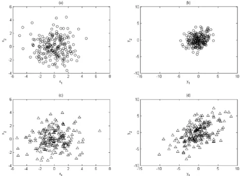
are zero vector, unity vector, and identity matrix, respectively. The scatter plots of these two realization sets are depicted in Figure 1, and these plots also implicitly show the significantly different principal directions of these two data sets, which are produced from the same system.
The ordinary PCA, modified PCA, and distance similarity measures evaluated from eqs 2, 3, and 8 for these two data sets are listed in the first column of Table 1. In this illustration, the operation level is changed. So, distance-based measure indicates very well the dissimilarity between the data sets. The other two measures also detect the dissimilarity. But they fail to tell if the change is resulted from input or from the process. Recall that these two data sets are from the same static processes.
2.3.2. Illustration 2. Let Z(1), Z(2) ∈ R200×4 designate two data sets with 200 samples and 4 variables in each, where the samples are collected from two different linear static processes as follows:
where B(1) ) [0.7 0.3; 0.2 0.8] and B(2) ) 2B(1) ) [1.4 0.6; 0.4 1.6].
In this example, one assumes that (x(1), x(2)) and (e(1), e(2)) are random vectors having the same probability distributions; they are designated by the following.
The scatter plots of these two realization sets are shown in Figure 2, and the PCA-based and distance-based similarity measures are evaluated using eqs 2, 3, and 8 and listed in the second column of Table 1. In this illustration, the model is changed. The PCA-based measures may interpret the change is from input magnitude. Because these measures are insensitive to the input magnitude, they indicate a high similarity as expected. The distance-based measure indicates that the operation level is
Figure 1. Scatter plots of illustration 1: (a, b) plots of data set 1 and (c, d) plots of data set 2. Table 1. PCA, Modified PCA, and Distance Similarity Measures for
Illustration 1 and Illustration 2
illustration 1 illustration 2
SPCA 0.8993 0.9224
SPCA
λ 0.2829 0.9255
Sdist 0.0494 0.9702
y(i)) Bx(i)+ e(i); B ) [0.7 0.3; 0.2 0.8]
z(i)) [y(i)Tx(i)T]T (9)
x(i)∼ N(µx(i), Σx (i) ) e(i)∼ N(µe(i), Σe (i) ) (10)
y(i)) B(i)x(i)+ e(i) z(i)) [y(i)Tx(i)T]T
(11)
x(1), x(2)∼ N(0, diag([3 2]))
e(1), e(2)∼ N(0, I)
unchanged only. That means they are difficult to detect or the source of change (i.e., model or input) is difficult to distinguish. 3. Parameter Similarities for Linear Static Processes
The following linear regression model is usually used to the describe linear functional relationship between input and output variables in static and multivariate processes.
or
where Y∈ RN×ny, X∈ RN×nx, B∈ RNx×ny, and E∈ RN×nyare the
response, effect, parameter, and residual matrices, respectively. The integers N, ny, and nx designate the number of samples, response variables, and effect variables, respectively. If the ordinary least-squares (OLS) method is applied to estimate these parameters, the parameter matrix and its variance structure estimates could be computed by the following24
in which the value σi2 could be estimated directly from the residual vector Eias follows:24,25
Let{X(I), Y(I)}and{X(II), Y(II)}denote two data sets with N I and NIIsamples, respectively. Their corresponding parameters and parameter variances, designated as B(k)andσ
i 2,(k)) [σ i1 2,(k) ‚‚‚ σinx 2,(k) ]T, i∈{1,‚‚‚,n
y}, k∈{I,II}, can be estimated directly using eq 15. A pooled parameter variance can be used to compare the similarity of parameters in different sets. Letσj2,(I,II)
denote the pooled variance of parameters βij(I) and βij(II). A pooled variance of the data sets is then defined as follows:22,26
Let Br(I,II) with elementsβ ij
r(I,II) be defined as the difference between B(I)and B(II); that is,
The hypothesis that βij(I) is similar to βij(II) can be tested by examining if the following inequality holds:
where σjij(I,II) is the pooled standard deviation of parameter
βijr(I,II)βij(I), and cv g0 is the threshold based on the selected confidence.
Then, a violating number is defined as follows:
whereδv(•) is a function which satisfies
Finally, the similarity measure of these two data sets I and II based on their characteristic parameters can be given by
In eq 22, ntis the total number of parameters in Br(I,II). In accordance with eqs 19 and 22, the features of this defined parameter similarity are listed as follows.
1. The range of this similarity is from zero to unity, that is,
Figure 2. Scatter plots of illustration 2: (a, b) plots of data set 1 and (c, d) plots of data set 2.
Y ) [y1y2‚‚‚ yn y] ) XB + E (13) yi) Xβi+ Ei, i∈{1,2,‚‚‚,ny} (14) B ) (β1,β2,‚‚‚,βn) ) (X TX)-1XTY var(βi) ) diag((X T X)-1σi 2 ) )σi2 (15) σi 2) 1 (N - nx)Ei TE i (16) σjij2,(I,II)) 1 NI+ NII- 2((NI- 1)σij 2,(I)+ (N II- 1)σij 2,(II)) (17)
Br(I,II) ) B(I)- B(II) (18)
-cvσjij(I,II)e βij r (I,II) e cvσjij (I,II) (19) nv(I,II) )
∑
j)1 nx∑
i)1 ny δv(|βijr(I,II)| - cvσjij (I,II) ) (20) δv(ξ) ){
1, if ξ g0 0, if ξ < 0 (21) Sstatic(I,II) ) 1 -n v (I,II) nt , nt) nx× ny (22) 0 e Sstatice 12. Multiplicative faults can be detected by this similarity. For instance, a process model change can be detected if Sstaticis not close to unity.
3. Dissimilar parameters of processes can be isolated using eq 19.
4. The difference or ratio of dissimilar parameters can be regarded as the fault magnitude in that parameter.
4. Parameters for Dynamic Processes
For a dynamic system, the process dynamics can be repre-sented by an expression similar to that of a static system. That is,
in which Yi is an output vector, matrix Hi is the parameter matrix, and Eiis the residual matrix. Matrix Hican be estimated from the sets of input and output data by the following:
where
and
Notice that i∈{1,2,‚‚‚,ny}, j∈{1,2,‚‚‚,nu}, and N ) 2m + n -1, which is the total number of samples. The number n should be much greater than the selected number m. The notation (•)†
is the pseudo-inverse operator for a matrix. Matrix Hijf is a lower triangular Toeplitz matrix as follows:
Define hij0as the transpose of the last row of Hijf in a reverse order, that is,
The last (m - 1) elements in parameter vector hij0 form the impulse response sequence from the jth input to the ith output.18,19
We take the transpose of eq 23 to yield
The above representation is similar to the equation form for static systems in eq 13. Let zi, Oi, and Eidenote the last column vectors of the matrices (Yif)T, H
i T
, and EiT, respectively. On the basis of eq 14, one can express zias
Similar to the analysis procedure for static processes in section 3, the variance structure ofφican be estimated using eq 15 as
where σj2 is the estimated variance of Ei, which can be evaluated using eq 16.
Let Σidesignate the estimated covariance matrix ofφi, that is,
Because hij 0
is a subset of φi from element (j - 1)m + 1 to element j× m in reverse order, the covariance structure of hij0 can be extracted from Σiby the following:
where rev(•) is defined as a reverse operator for a matrix as
Let hij be the last m - 1 elements of hij 0
, and then it is the impulse sequence of the jth input and the ith output of this process, that is,
Similarly, the covariance and variance structures for hij could be expressed as follows: Yi) HiΓi+ Ei (23) Hi) YiΓi T (ΓiΓi T)† (24) Γi) [(U1 f)T‚‚‚ (U nu f )T| (U l p)T‚‚‚ (U nu p)T| (Y i p)T]T ∈ R(2nu+1)m×n Hi) [Hi1f ‚‚‚ Hin u f | H i1 p ‚‚‚ H inu p | H i0 p]T∈ Rm×(2nu+1)m Yip)
[
yi(1) yi(2) ‚‚‚ yi(n) yi(2) yi(3) ‚‚‚ yi(n + 1) l l ‚‚ ‚ l yi(m) yi(m + 1) ‚‚‚ yi(m + n - 1)]
∈ Rm×n Yif)[
yi(m + 1) yi(m + 2) ‚‚‚ yi(m + n) yi(m + 2) yi(m + 3) ‚‚‚ yi(m + n + 1) l l ‚‚ ‚ l yi(2m) yi(2m + 1) ‚‚‚ yi(2m + n - 1)]
∈ Rm×n Ujp)[
uj(1) uj(2) ‚‚‚ uj(n) uj(2) uj(3) ‚‚‚ uj(n + 1) l l ‚‚ ‚ l uj(m) uj(m + 1) ‚‚‚ uj(m + n - 1)]
∈ Rm×n Ujf)[
uj(m + 1) uj(m + 2) ‚‚‚ uj(m + n) uj(m + 2) uj(m + 3) ‚‚‚ uj(m + n + 1) l l ‚‚ ‚ l uj(2m) uj(2m + 1) ‚‚‚ uj(2m + n - 1)]
∈ Rm×n (25) Hijf )[
0 0 ‚‚‚ 0 0 hij(1) 0 ‚‚‚ 0 0 hij(2) hij(1) ‚‚‚ 0 0 l l ‚‚ ‚ l l hij(m - 1) hij(m - 2) ‚‚‚ hij(1) 0]
∈ Rm×m (26) hij0) [0 hij(1) ‚‚‚ hij(m - 1)]T∈ Rm (27) (Yif)T) ΓiTHiT+ EiT ) Γi T [(Hi1 f )T‚‚‚ (Hinu f )T| (Hi1 p )T‚‚‚ (Hinu p )T| (Hi0 p )T]T+ Ei T (28) zi) ΓiTφi+ Ei (29) var(φi) ) diag((ΓiΓi T )†σi 2 ) (30) Σi) (ΓiΓi T )†σi 2 (31) cov(hij0) ) rev(Σi((j - 1)m + 1:j× m, (j - 1)m + 1:j × m)) (32) rev(
[
a11 a12 ‚‚‚ a1q a21 ‚‚‚ ‚‚‚ l l l ‚‚ ‚ l ap1 ‚‚‚ ‚‚‚ apq]
)
)[
apq ap(q-1) ‚‚‚ ap1 a(p-1)q ‚‚‚ ‚‚‚ l l l ‚‚ ‚ l a1q ‚‚‚ ‚‚‚ a11]
(33) hij0) [0 hijT]T (34)The averaged parameter variance for all elements in hijcan be given by
The process dead time for sub-model (i,j), designated as dij, is taken as the integer k such that
where σij ) xσij 2
and cv is the threshold with prescribed confidence.
When using the aforementioned criterion to specify dead times, the resulting dead times will be sensitive to outliers at the very beginning of the computed hijsequence. A more robust estimation for this process dead time in sub-model (i,j) can be determined as follows.
On the basis of the aforementioned derivations, a nonparametric model for a dynamic system can be evaluated. Some features of this mathematical representation include the following:
1. The model structure does not need to be known in advance. 2. The number of parameters m in a model is adjustable for required accuracy or available observations of measurements. 3. The dead times of processes can be estimated straightfor-wardly from the evaluated parameter vectors.
4. The corresponding variances of parameters can be analyti-cally estimated using the conventional regression analysis. 5. Similarity Measures for Dynamic Processes
In this section, a variety of definitions of similarities between dynamic processes will be proposed. They can be basically classified into two categories, overall similarity and the sub-model similarities. The overall similarity is a lumped overall assessment of a dynamic model that consists of several sub-models, and the sub-model similarities refer to similarities specific to each sub-model. Moreover, resolution-enhanced overall and sub-model similarities will also be developed using a weighted factor method. Because identification of a process model with closed-loop data is still an open problem, the estimation of parameters in a dynamic system (e.g., eq 23) requires open-loop pseudo-random binary sequence (PRBS) input excitations. Nevertheless, these PRBS excitations may be incorporated into a closed-loop system so that the fault detection and isolation can be carried on without drastically disturbing the system. This will be addressed later.
Let {U(I), Y(I)}and{U(II),Y(II)}be two dynamics data sets with sample number NIand NIIat run I and run II, respectively. Assume the sampling time of these two sets is the same. Using eq 24, one can compute their characteristic parameter vectors from each input and output pair. Moreover, the variance and covariance structures are estimated through eq 35 to yield
where k ∈{I,II}, i∈{1,2,‚‚‚,ny}, and j ∈{1,2,‚‚‚,nu}. In this study, one assumes the number of elements computed in each impulse sequence from run I and run II is equal to m.
From eq 23, the output yiat time instant k can be expressed as follows:
where uj(k) ) [uj(k - 1) ‚‚‚ uj(k - m)]Tand gi(k) is the residual.
5.1. Overall Similarity. To define the overall similarity, a pooled variance of parameters hij(I) and hij(II) is first estimated using the data from run I and run II. That is,22
Furthermore, the scaled parameter vector hhij using the pooled variance is then defined in eq 42:
where hhij(k)) hij(k)× (σjij(I,II))-1andσjij(I,II) ) (σjij2,(I,II))1/2.
The deviations of the two sets of parameters are then computed directly using eq 43.
Consequently, the violating number nij v
(I,II) for sub-model (i,j) between run I and run II can be counted as follows:
whereδv(•) is an index function which has been specified in eq 21 and cvis a threshold with a specified confidence level. Notice that the residues are weighted withω, 0 e ω e 1. The
resolution of similarity measures between hij(I)and hij(II)can be enhanced by this weight assigned to the parameters. In eq 44, the residues in eq 43 are weighted into two parts. The residues in the first part are usually weighted more than those in the second part. The number of terms in the first part is determined by a cutoff number mijwhich is defined as the following:
where Σij) cov(hij) ) rev(Σi((j - 1)m + 1:j× (m - 1), (j - 1)m + 1:j × (m - 1)))∈ R(m-1)×(m-1) (35) σij2) var(hij) ) diag(Σij)∈ Rm-1 σij 2) 1 m - 11 T σij 2 (36) dij) k if |hij(k)| e cvσij and |hij(k + 1)| > cvσij (37) dij) k if |hij(k)| e cvσij and |hij(k + 1)|,|hij(k + 2)| > cvσij (38) H(k)) [h11(k)‚‚‚ hij(k)‚‚‚ hn ynu (k) ]∈ Rm(k)×(nynu) var(hij(k)) )σij2,(k) and σij2,(k)) 1 m(k) 1Tσij2,(k) (39) cov(hij(k)) ) Σij (k) yi(k) )
∑
j)1 nu {hijTuj(k)}+ gi(k) (40) σjij 2,(I,II)) 1 NI+ NII- 2((NI- 1)σij 2,(I)+ (N II- 1)σij 2,(II) ) (41) Hh(k)) [hh11(k)‚‚‚ hhn ynu (k) ], k∈{I,II} (42)Hhr(I,II) ) Hh(I)- Hh(II) (43)
nijv(I,II) )
∑
k)1 mij(I) (δv(|hhij r (k)| - cv)× ω) +∑
k)mij(I)+1 m (δv(|hhij r (k)| - cv)× (1 - ω)) (44) Eij(mij) Eij(m) g λ and Eij(mij- 1) Eij(m) < λ (45) Eij(l) )∑
k)1 l {hij(k)}2 (46)andλ is a number between 0 and 1. The factor ω is usually
assigned to be greater than 0.5 because a heavier weight on the first part is desirable.
Finally, the total violating number nv(I,II) for whole param-eters in Hhr(I,II) becomes
The overall similarity between data set I and data set II can be expressed as
in which nt,(I)is the weighted number of parameters in Hhr(I,II) as defined by
Note here that the values of St(I,II) and St(II, I) may be different because mij(I) and mij(II) may be different. The main purpose of the overall similarity is to detect the occurrence of multiplicative faults in a dynamic system. If the value St(I,II) is not close enough to unity, this indicates that the process has changed between run I and run II.
5.2. Sub-Model Similarities. 5.2.1. Similarity for Detection of Sub-Model Changes. The similarity measure of sub-model (i,j) is defined for each dynamic element in the process. Similar to the overall similarity, it is defined as follows:
The main purpose of this similarity measure is to isolate which sub-model has faults. If Sij(I,II) is far from unity, there is potential process model change in sub-model (i,j). On the contrary, the possibility of the existence of a multiplicative fault in sub-model (i,j) is low if Sij(I,II) is very close to unity.
5.2.2. Similarity for Detection of Dead Time Change. In this subsection, the similarity on two dead-time-free parameter vectors hij(I)and hij(II)will be defined. Let vectors hij(I),dand hij(II),d denote the dead-time-free parameter vectors after exclusion of dead time, and they are all cut short to have an equal number of elements, mijd, so that hij(I),d, hij(II),d∈ Rmijd
.
Then, the scaled parameter vectors using pooled variance are computed as
Similarly, the corresponding residual vector is as
Because the dead time elements in hij have been removed in the construction of hijd, the corresponding separation point mij should be shifted by the following.
Consequently, the violating number for sub-model (i,j) after dead time exclusion could be redefined using the format of eq 44:
Finally, the similarity on the dead-time-free sub-models (i,j) would be
The major usage of this similarity measure is to detect possible dead time changes in the sub-model (i,j). In this case, a change will lead to an Sij(I,II) far from unity and an Sij
d(I,II) close to unity. The magnitude of this fault in dead time can be estimated as
5.2.3. Similarity for Detection of Gain Changes. This similarity measure is used to identify the change of gain in sub-models (i,j). The process gain is estimated by the sum of all elements in an impulse response sequence assuming that m approaches infinity. For sequence hij, let Kijdesignate a scaled factor as follows.
Then, the original parameter vectors are scaled using the above scaled factors as
where i∈{1,2,‚‚‚,ny}and j∈{1,2,‚‚‚,nu}. Because the original vector is scaled by a constant factor, its corresponding parameter and averaged parameter variances become
Consequently, the pooled variance of these gain scaled parameter vectors would be expressed as
Finally, scale the dead-time-free part of the vectors using their pooled variance to obtain hhij(k),Kd:
It should be noted that the lengths of hhij (I),Kd
and hhij (II),Kd
are all truncated to have the same number mijd. The corresponding residuals are nv(I,II) )
∑
j)1 nu∑
i)1 ny nijv(I,II) (47) St(I,II) ) 1 -n v (I,II) nt,(I) (48) nt,(I))∑
j)1 nu∑
i)1 ny (mij(I)× ω + (m - mij(I))× (1 - ω)) (49) Sij(I,II) ) 1 - n v (I,II) mij(I)× ω + (m - mij(I))× (1 - ω) (50) hhij(k),d) hij(k),d× (σj(I,II)ij )-1, k∈{I,II} (51) h h ij r,d(I,II) ) hhij(I),d- hhij(II),d (52)
mijb) mij- dij (53) nijv,d(I,II) )
∑
k)1 mijb,(I) (δv(|hhij r,d (k)| - cv)× ω) +∑
k)mijb,(I)+1 mijd (δv(|hhij r,d (k)| - cv)× (1 - ω)) (54) Sijd(I,II) ) 1 - nij v,d(I,II) mijb,(I)× ω + (mijd- mijb,(I))× (1 - ω) (55)dijf(I,II) ) dij(I)- dij(II) (56)
Kij)
∑
k)1 mij {hij(k)× ω}+∑
k)mij+1 m {hij(k)× (1 - ω)} (57) hijK) hij× (Kij)-1 (58) σij2,K) σij2× (Kij)-2 σij 2,K) σ ij 2× (K ij) -2 (59) σjij2,(I,II),K) 1 NI+ NII- 2((NI- 1)σij 2,(I),K+ (N II- 1)σij 2,(II),K ) (60) hhij(k),Kd) hij(k),d× (σj(I,II),Kij )-1 k∈{I,II} (61)Thus, the violating number of these dead-time-free vectors can be determined by
Likewise, the similarity for detection of gain changes is given as
If Sij(I,II) and Sij
d(I,II) are all far from unity but S ij
Kd(I,II) is close to unity, the change of gain in the sub-model (i,j) will be isolated. The magnitude of this fault in the gain can be estimated as
Some basic features of these defined similarities for dynamic processes are summarized as follows:
1. The range of these similarities are all from zero to unity, that is,
2. Multiplicative faults can be detected using overall similarity St.
3. Abnormal subsystems can be isolated by sub-model similarity Sij.
4. Changes in dead times of a process can be identified from the similarity Sijd.
5. Changes in gains of a process can be identified from the similarity SijKd.
In summary, after defining these similarity measures for process characteristics, a unified multiplicative fault detection, isolation, and identification procedure via these indices is proposed in the following steps.
1. Identify the parameters of process H(k)and estimate their variance and covariance structures σij(k) and Σij(k) using the methods describe in section 4 for the given data pairs {U(k),
Y(k)}, where k∈{I,II}, i∈{1,‚‚‚,n
y}, and j∈{1,‚‚‚,nu}. Go to step 2.
2. If the overall similarity St(I,II) is not close to unity, a possible multiplicative fault exists in whole system. Go to step 3 for fault isolation.
3. If sub-model similarity Sij(I,II) is not close enough to unity, a process change exists in sub-model (i,j) has been isolated; go to step 4 for process dead time fault identification. Otherwise go to step 6.
4. If the similarity Sij d
(I,II) is close enough to unity, a fault related to the dead time in sub-model (i,j) is identified. Its magnitude can be estimated using eq 56. Then go to step 6. Otherwise go to step 5 for process gain fault identification.
5. If the similarity SijKd(I,II) is close to unity, a process gain fault in sub-model (i,j) is identified, and its magnitude can be estimated by eq 65. Go to step 6. Otherwise a process change related to dynamics or a mixture of dead time, gain, and dynamic characteristics is identified. For the multiplicative fault related to the change of dynamics, a parsimonious process model might be required for identifying the corresponding root causes.
6. Repeat steps 3-5 until all pairs of impulse sequences of sub-models are all examined.
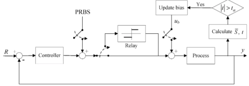
6. Extensions to On-Line Process Change Diagnosis The similarity measures between dynamic data sets described in section 5 can be easily performed for on-line multiplicative fault diagnosis. In this section, a procedure for on-line imple-mentation procedure will be presented in detail. As mentioned previously, the estimation of parameters needs open-loop PRBS excitations. These PRBS excitations can be generated by the system as shown in Figure 3. The conventional loop monitors the output during start-up or when a large disturbance occurs. When the system output is controlled within a normal region around its target value, the control task can be taken over by the second loop which monitors the mean of the output. A PRBS signal is introduced, and the relay is activated. The PRBS has a large magnitude to override the algebraic sign of the summed input to the relay and give a smaller PRBS output in turn to excite the process for parameter estimations. In this way, the process is under control while the process is excited by a substantial PRBS input. The data can then be collected for similarity evaluation on the basis of the presented method. Anytime during the on-line stage, if the system detects a trend of mean change in terms of a Student t test (e.g., t > tR), that means the process has been subjected to some unknown disturbance or process change. Upon this, the outer loop will be monitoring this mean and produce proper bias to the relay to compensate for the change and bring the mean back to zero. The compensating bias in the relay indicates that some fault has occurred. A new set of parameters together with their variance/covariance matrices can be calculated, and the similar-ity indices can be applied. This identification process has been demonstrated in a paper by Jeng and Huang.19In the following, the on-line implementation of the fault detection and isolation will be addressed.
Figure 3. External loop incorporated to a conventional control system for PRBS excitation.
nijv,Kd(I,II) )
∑
k)1 mijb,(I) {δv(|hhij r,Kd (k)| - cv)× ω}+∑
k)mijb,(I)+1 mijd {δv(|hhij r,Kd (k)| - cv)× (1 - ω)} (63) SijKd(I,II) ) 1 - nij v,Kd(I,II) mijb,(I)× ω + (mijd- mijb,(I))× (1 - ω) (64) Kijf(I,II) )Kij (I) Kij(II) (65) 0 e St, Sij, Sij d , SijKde 1The first step toward on-line implementation is the identifica-tion of the parameters and their variance and covariance structures from a given normal operating data set as a benchmark.
where U(0) and Y(0) are the input and output data matrices, respectively, from a nominal process with N samples, that is,
The parameters, variances, and covariance are estimated from a data set with N samples at time instant k for a similarity check with the benchmark model, that is,
where
For simplicity, the parameter variance and covariance structures are adopted from those of normal data to reduce the computa-tional cost. In other words,
If necessary, the recursive least-squares algorithm could be applied to eqs 68 and 70 to evaluate the corresponding impulse sequences iteratively.24,27Then, the following similarity mea-sures can be computed directly from their definitions as mentioned in the previous section.
Finally, on-line updating of these measures can be imple-mented based on the similarity measures.
Remarks. 1. Because we need redundant impulse sequences obtained from normal cases for estimating the statistics of similarity measures, the greater the number of redundant
sequences the better. But, from statistical point of view, three to five should be required at least.
2. The number of samples should be greater than the parameters that can sufficiently represent the dynamics in the system.
3. In general, it is suggested that the sampling rate should not greater than 1/10 of the smallest time constant in the system. 7. Illustrative Examples
In this section, two simulated case studies are used to demonstrate the efficacy of the presented multiplicative fault diagnosis approach. The first case is a non-squared numerical multi-input multi-output (MIMO) system with different sce-narios of parameter changes, and the proposed parameter similarity measures are applied to identify the root causes of abnormalities. In the second application, the developed on-line process change monitoring procedure is conducted on an industrial 2 × 2 distillation process. From the corresponding monitoring charts of parameter similarities, the multiplicative faults can be detected, isolated, and identified. The processes in these illustrative case studies are all assumed to be operated under open-loop excitations for convenience. If the process model can be identified with feedback controls using some closed-loop process identification algorithm, the introduced multiplicative faults in these systems could also be detected and isolated directly with the use of these proposed parameter similarity measures.
7.1. Example 1. A transfer function model is frequently used as a basic description of a dynamic system for a variety of purposes, such as controller design, process control, control performance assessment28,29and data reconciliation, and so forth. In this example, a 4× 2 dynamic system (two inputs and four outputs) with the following nominal transfer function matrix is considered.
The nominal dynamic process is expressed as follows:
where y(s), u(s), and e(s) are outputs, inputs, and measurement errors, respectively. Assuming that the measurement errors follow independently and identically distributed (i.i.d.) Gaussian distributions with zero mean and unit variance, that is, e ∼
N(0,I) and assuming that the nominal plant is excited with
normally distributed random inputs,
Table 2. Fault Scenario for Example 1 (2× 4 Numerical Case)
transfer function fault type nominal faulty transfer function fault type nominal faulty
G11 N/A N/A N/A G12 N/A N/A N/A
G21 dead time 6 8 G22 dead time 11 7
G31 gain -5 -10 G32 gain -20 -10 G41 dynamics 6s + 1 12s + 1 G42 dynamics 18s + 1 10s + 1 G0(s) )
[
3(6s + 1) (3s + 1)(10s + 1)e -s 10(25s + 1) (5s + 1)(50s + 1) 10 (2s + 1)2e -6s 12 (5s + 1)2e -11s -5 (5s + 1)(3s + 1)e -5s -20 (8s + 1)(2s + 1)e -3s 15 6s + 1e -2s -30 18s + 1e -5s]
(75)y(s) ) G0(s) u(s) + e(s) (76)
u0∼ N
(
0,[
3 0 0 2]
)
(77) {U(0),Y(0),m}98parameters estimation {H (0),{ σ11(0)‚‚‚ σn ynu (0)},{ Σ11 (0)‚‚‚ Σ nynu (0)}} (66)U(0)) [u(0) u(1) ‚‚‚ u(N - 1)]T∈ RN×nu
Y(0)) [y(0) y(1) ‚‚‚ y(N - 1)]T∈ RN×nu
(67) {U(k),Y(k),m}98full para.est. {H (k),{ σ11(k)‚‚‚ σn ynu (k) },{ Σ11 (k)‚‚‚ Σ nynu (k) }} (68)
U(k)) [u(k) u(k + 1) ‚‚‚ u(k + N - 1)]T∈ RN×nu
Y(k)) [y(k) y(k + 1) ‚‚‚ y(k + N - 1)]T∈ RN×nu
(69) {U(k),Y(k),m}98simplified para.est. {H (k)} (70) 1. Overall similarities St0(k) ) St(0,k) (71) 2. Similarities for isolation of sub-models
Sij0(k) ) Sij(0,k) (72) 3. Similarities for detection of dead time changes
Sij0,d(k) ) Sijd(0,k) (73) 4. Similarities for detection of gain changes
The sampling time is set as 1 s, and 600 samples are collected from this nominal system during the excitation period. A list of the process changes is given in Table 2, and Gijrefers the entry (i,j) in eq 75. Consequently, the corresponding transfer function matrix of the faulty system would be as follows:
For diagnosing multiplicative faults, the inputs for this case are
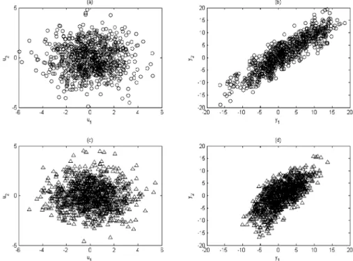
A total of 500 realizations are collected as comparative samples, and the scatter plots of the data sets from the nominal and the faulty systems are shown in Figure 4. The signal structure of the measurement errors and the sampling time for the faulty system (eq 78) are all assumed to be the same as the those of the nominal system (eq 75).
The similarity measures with factors m ) 30,λ ) 0.75, and ω ) 0.9 are prescribed to analyze these two data sets (nominal
and faulty). The evaluated overall similarity is 0.5095, and this index shows that the parameters of these two sets are different. One might conclude that there exists process changes in this plant using this index. The remaining sub-model similarities for subsystems in this process are listed in Table 3. From the first row of Table 3, the sub-model similarity measures for G11
and G12are equal to 1, and it shows that these two subsystems are normal. On the contrary, the other sub-model similarities are not close to unity, and multiplicative faults, which exist in G21, G22, ..., G42must be isolated one by one.
After removing the dead time elements from the correspond-ing parameter vectors, the similarities for detection of dead time changes, that is, row 2 of Table 3, indicate that subsystems G21 and G22have different dead times because their corresponding similarity measures are close to unity after removal of the dead time. The evaluated fault magnitudes using eq 56 are -2 and 4 s for G21and G22, respectively.
Furthermore, if parameter vectors are scaled down using their associated gain scaling factors, the similarities for detection of gain changes (row 3, Table 3) reveal that the gain has changed in subsystems G31and G32. The estimated fault magnitudes using eq 65 are 0.4923 and 1.8157 for G31and G32, respectively.
Because no proposed similarity measure can improve the similarities of G41and G42, one might conclude that the dynamic characteristics of these two subsystems are substantially dif-ferent.
7.2. Example 2. Wood and Berry30presented a 2× 2 transfer function model for a distillation column to separate methanol and water (WB system). The two outputs are the mole fraction of methanol in the distillate and in the bottom. The two inputs are the reflux flow and vapor boil-up rate, respectively. The following WB column system is used to produce the simulated data:
Consequently, the nominal dynamic process can be expressed as follows:
where y(s), u(s), and e(s) are outputs, inputs, and measurement errors, respectively. In this case, the measurement errors are i.i.d. Gaussian random variables with zero mean and variance 0.5, that is, e∼ N(0,0.5I).
Figure 4. Scatter plots of example 1: (a-c) plots of the nominal data set and (d-f) plots of the faulty data set. Table 3. Sub-Model Similarities for Diagnosing Multiple
Multiplicative Faults in Example 1 (2× 4 Numerical Case Study)
G11 G12 G21 G22 G31 G32 G41 G42 Sij 1 1 0.6091 0.4899 0.3433 0.2857 0.3721 0.4241 Sij d 1 1 1 1 0.1124 0.1633 0.2059 0.1947 SijKd 1 0.8714 1 1 1 0.9082 0.1618 0.3540 G*(s) )
[
3(6s + 1) (3s + 1)(10s + 1)e -s 10(25s + 1) (5s + 1)(50s + 1) 10 (2s + 1)2e -8s 12 (5s + 1)2e -7s -10 (5s + 1)(3s + 1)e -5s -10 (8s + 1)(2s + 1)e -3s 15 12s + 1e -2s -30 10s + 1e -5s]
(78) u*∼ N(
[
1 1]
,[
5 -4 -4 4]
)
(79) G(s) )[
12.8 16.7s + 1e -s -18.9 21s + 1e -3s 6.6 10.9s + 1e -7s -19.4 14.4s + 1e -3s]
(80)This process is assumed to be operated under supervised open loop conditions and be continuously excited by a sequence of Gaussian random variables. The input is given as follows.
Other basic properties of this system are as follows: 1. Sampling time is set as 1 s.
2. A total of 1800 observations (including nominal and faulty data) are collected.
After operating normally for 800 s, some multiplicative changes, as listed in Table 4, are introduced at time instant 800. The scatter plots of the nominal data set (800 realizations) and the faulty data set (1000 realizations) are shown in Fig-ure 5.
The first 600 samples of data are used to identify the system parameter vectors and to specify the parameter variances, that is,
Figure 5. Scatter plots of example 2: (a, b) plots of the nominal data set and (c, d) plots of the faulty data set.
Figure 6. Overall similarity for example 2 (WB process).
Table 4. Fault Scenario for Example 2 (WB System)
transfer function fault type nominal faulty transfer function fault type nominal faulty
G11 dead time 1 7 G12 gain -18.9 -9.5
G21 dynamics 10.9s + 1 21s + 1 G22 N/A N/A N/A
u∼ N
(
0,[
3 00 2
]
)
(82)A moving-window approach is used to collect the corre-sponding data sets at a specific time instant, and the parameter vectors are also estimated for them, that is,
Because of this, one finds the following:
1. If k e 200, the collected data are all nominal.
2. If 200 < k e 800, the faulty data start to enter the collected data set to replace some of the normal data.
3. If k > 800, the collected data are all faulty.
It should be noted here that simplified parameter estimation (eq 70) is used in this example. In this case, similarity measures
with factors m ) 30,λ ) 0.75, and ω ) 0.9 are prescribed to
compare the parameter vectors at time instant k and 0. The evaluated overall similarity is depicted in Figure 6, and it shows that the change of process model begins around k ) 200. Figure 7 shows the sub-model similarity for these four subsystems. The multiplicative faults are correctly and clearly isolated in G11, G12, and G21. After the transition period 200 <
k e 800, the similarities for identification of dead time changes, which are illustrated in Figure 8, show that the type of fault in G11is the change of dead time. Likewise, the similarities for identification of gain changes in Figure 9 illustrate that the fault in G12is a change of gain after the transition period 200 < k e 800. Because no proposed sub-model similarity measure can make the similarity of G21close to unity, one might conclude
Figure 7. Sub-model similarities for isolating faulty subsystems for example 2 (WB process).
Figure 8. Similarities for identifying dead time changes for example 2 (WB process).
that there was a change of process dynamics in the subsystem G21. On the contrary, the sub-model similarities for G22are all close to unity as seen from Figures 7-9; this clearly shows that the subsystem G22has no multiplicative fault.
8. Conclusions
The safety and performance of an industrial plant are important subjects for research. Among these, changes in the operation conditions and process dynamics of a system are important information for the operation and control of a plant. Any prompt and automatic detection and isolation of such process changes (or faults) from the recorded measurements will be beneficial. Currently, multiplicative faults of a system are usually diagnosed using a model-based approach. This approach is difficult for systems whose process model cannot be ac-curately identified and is restricted to some special model formats. Moreover, conventional similarity measures do not take into account the dynamics of the process and are not applicable to analyze the faults relevant to process dynamics. In this paper, a variety of parameter similarity measures are defined for detection, isolation, and identification of such dynamic faults. With the use of these defined parameter similarity indices, a unified fault diagnosis procedure is developed to analyze the possible root causes of process changes. In addition, this proposed diagnostic procedure can be implemented on-line for the purpose of real-time multiplicative fault monitoring. This proposed method has been tested with two simulated applica-tions with good performance in handling multiple and multi-plicative faults. Notice that the simple PCA-based approaches do not require system excitation but have limited capability in fault detections. This presented approach provides a unified and efficient solution for multiplicative fault diagnosis in multivariate dynamic systems. It requires more computations and system excitation and, thus, offers more. It can be a complement to the existing PCA-based measures to have a wider application range in terms of fault detections.
Literature Cited
(1) Li, W.; Shah, S. Structured residual vector-based approach to sensor fault detection and isolation. J. Process Control 2002, 12 (3), 429-443. (2) Qin, S. J.; Li, W. Detection and identification of faulty sensors in dynamic processes. AIChE J. 2001, 47 (7), 1581-1593.
(3) Li, C. C.; Jeng, J. C.; Huang, H. P. Multiple sensor fault diagnosis for dynamic processes. Comput. Chem. Eng. 2006, submitted.
(4) Basseville, M.; Nikiforov, I. Detection of abrupt changes - theory
and applications; Prentice Hall: New York, 1993.
(5) Gertler, J. Fault detection and diagnosis in engineering systems; Marcel Dekker: New York, 1998.
(6) Faloutsos, C.; Ranganathan, M.; Manolopoulos, Y. Fast subsequence matching in time series databases. Sigmod Record 1994, 23, 419-429.
(7) Keogh, E.; Chakrabarti, K.; Pazzani, M. Dimensionality reduction for fast similarity search in large time series databases. Knowl. Info. Syst.
2001, 3, 263-286.
(8) Krzanowski, W. J. Between-groups comparison of principal com-ponents. J. Am. Stat. Assoc. 1979, 74 (367), 703-707.
(9) Singhal, A.; Seborg, D. E. Pattern Matching in Historical Batch Data using PCA. IEEE Control Syst. Mag. 2002, 22 (5), 53-63.
(10) Johannesmeyer, M. C.; Singhal, A.; Seborg, D. E. Pattern matching in historical data. AIChE J. 2002, 48 (9), 2022-2038.
(11) Singhal, A.; Seborg, D. E. Pattern Matching in Multivariate Time Series Databases using a Moving-Window Approach. Ind. Eng. Chem. Res.
2002, 41, 3822-3838.
(12) Kano, M.; Hasebe, S.; Hashimoto, I.; Ohno, H. Statistical process monitoring based on dissimilarity of process data. AIChE J. 2002, 48 (6), 1231-1240.
(13) Singhal, A.; Seborg, D. E. Clustering multivariate time-series data.
J. Chemom. 2005, 19, 427-438.
(14) Li, W.; Jiang, J. Isolation of parametric faults in continuous-time multivariable systems: a sampled data-based approach. Int. J. Control 2004,
77 (2), 173-187.
(15) Isermann, R. Process fault detection based on modeling and estimation methods - a survey. Automatica 1984, 20, 387-404.
(16) Benveniste, A.; Basseville, M.; Moustakidges, G. The asymptotic local approach to change detection and model validation. IEEE Trans.
Autom. Control 1987, 32, 583-592.
(17) Gertler, J.; Kunwer, M. Optimal residual decoupling for robust fault diagnosis. Int. J. Control 1995, 61, 395-421.
(18) van Overschee, P.; de Moor, B. N4SID: subspace algorithms for the identification of combined deterministic-stochastic systems. Automatica
1994, 30 (1), 75-93.
(19) Jeng, J. C.; Huang, H. P. Model-based autotuning systems with two-degree-of-freedom control. J. Chin. Inst. Chem. Eng. 2006, 37 (1), 95-102.
(20) Jackson, J. E. A user’s guide to principal components; John Wiley & Sons: New York, 1991.
(21) Russell, E.; Chiang, L. H.; Braatz, R. D. Data-driven methods for fault detection and diagnosis in chemical processes. Springer: London, 2000. (22) Johson, R. A.; Wichern, D. W. Applied multiVariate statistical
analysis, 4th ed.; Prentice Hall: Upper Saddle River, NJ, 1998.
(23) Maesschalck, R. D.; Jouran-Rimbaud, D.; Massat, D. L. The Mahalanobis distance. Chemom. Intell. Lab. Syst. 2000, 50, 1-18.
(24) Seber, G. A. F. Linear regression analysis; John Wiley & Sons: New York, 1977.
(25) Rencher, A. C. Methods of multiVariate analysis, 2nd ed.; Wiley-Interscience: New York, 2002.
(26) Sheskin, D. Handbook of parametric and nonparametric statistical
procedures, 2nd ed.; Chapman & Hall: New York, 2000.
(27) Hsia, T. C. System identification: least-squares methods; Lexington Books: Lanham, MD, 1977.
(28) Huang, H. P.; Lee, M. W.; Chen, C. L. Inverse-based design for a modified PID controller. J. Chin. Inst. Chem. Eng. 2000, 31, 225-236.
(29) Huang, H. P.; Jeng, J. C. Monitoring and assessment of performance for single loop control systems. Ind. Eng. Chem. Res. 2002, 41, 1297-1309.
(30) Wood, R. K.; Berry, M. W. Terminal composition control of a binary distillation column. Chem. Eng. Sci. 1973, 28, 1707-1717.
ReceiVed for reView August 24, 2006 ReVised manuscript receiVed April 9, 2007 Accepted April 11, 2007