基於電腦視覺之即時穩健的泛型障礙物與車道偵測行車系統

國

立

交

通

大

學

電機與控制工程學系

碩

士

論

文

基於電腦視覺之即時穩健的

泛型障礙物與車道偵測行車系統

A Real-Time Robust On-Vehicle

Generic Obstacle and Lane Detection System

Based on Computer Vision Technique

研 究 生：賴則全

指導教授：吳炳飛 教授

Detection System Based on Computer Vision Technique

研 究 生：賴則全 Student：Tze-Chiuan Lai

指導教授：吳炳飛 Advisor：Bing-Fei Wu

國 立 交 通 大 學

電 機 與 控 制 工 程 學 系

碩 士 論 文

A Thesis

Submitted to Department of Electronic and Control Engineering College of Electrical Engineering and Computer Science

National Chiao Tung University in partial Fulfillment of the Requirements

for the Degree of Master

in

Electronic and Control Engineering July 2005

Hsinchu, Taiwan, Republic of China

學生：賴則全

指導教授：吳炳飛 博士

國立交通大學電機與控制工程學系 碩士班

摘

要

近年來隨著交通問題日益嚴重，智慧型運輸系統(Intelligent transportation system, ITS) 的相關研究愈來愈受到重視，其中智慧型車輛又是最有發展潛力的研究之一。而泛型障 礙物與車道偵測系統是智慧車所需配備的最基本功能，能夠偵測出路面障礙物的位置與 車道資訊，用以預警駕駛人注意或者提供車輛自動行駛所必需的道路資訊。 本文主要是利用影像處理與電腦視覺的技術去偵測路上障礙物與車道的位置。將兩 支單色CCD 攝影機分別上下地架設在車上，利用 histogram-based 的方法將上方攝影機 所擷取出的道路影像做分類，以偵測出不同類別的交界所組成之近乎水平的邊線。所偵 測出的邊線可能位於地面或者障礙物上，這兩種情況判斷的依據是藉由立體視覺的技術 分別預估此邊線在下方影像中可能是地面的位置以及可能是障礙物的位置，然後量測與 上方影像中之邊線的相關係數何者比較大來做判斷，因此可以鑑別出影像中障礙物與路 面的部分。 而在車道偵測方面，使用一支單色 CCD 攝影機擷取道路影像，以偵測車道標線的 位置。本文所發展出的車道偵測演算法是基於車道幾何模型的標線偵測方式，能夠提供 一個穩健的偵測結果，並且適當地預估與縮小搜尋範圍，以降低搜尋時間而提高車道偵 測的效率。最後並重建車道3-D 幾何模型以修正道路傾斜度與寬度，因此本文所提出的 演算法亦適用於非平坦的路面。

結合方向盤控制器，做為無人駕駛智慧車的視覺系統，完成台灣第一台可以 hand-free 自動駕駛的智慧車TAIWAN iTS-1。TAIWAN iTS-1 以時速 90 km/hr 與 110 km/hr 分別

在東西向快速道路與國道3 號高速公路順利地自動駕駛實車測試，並經過國外卓越計畫

A Real-Time Robust On-Vehicle Generic Obstacle and Lane

Detection System Based on Computer Vision Technique

student：Tze-Chiuan Lai

Advisor：Dr. Bing-Fei Wu

Department of Electronic and Control Engineering

National Chiao Tung University

ABSTRACT

As the traffic is becoming more and more serious in most developed countries, a lot of researches about the intelligent transportation system (ITS) have been paid attention in recent years. Above all, one of the most promoting topics for the ITS applications is concerning the smart vehicles. The fundamental function of the smart vehicle is the generic obstacle and lane detection system, which can warn the driver or provide the road information for the unmanned vehicle.

In this thesis the techniques of image processing and computer vision are applied to the detection system. Two monochromatic CCD cameras are mounted top and bottom on the vehicle, and the road image captured by the top camera is segmented by thresholding the histogram. After that, the quasi-horizontal boundaries formed by the interconnection of two different segments are detected in order, and each detected boundary could belong to either the ground or the obstacle. The criterion to distinguish between them is to predict the corresponding ground and obstacle boundaries in the bottom image by the stereo vision, and to compute the normalized correlation coefficients of the detected boundary in the top image with respect to the ground and obstacle boundaries in the bottom image respectively. The detected boundary in the top image belongs to the obstacle if the normalized correlation coefficient associated with the obstacle is larger than that associated with the ground. Thus the road image can be divided into the ground and obstacle parts.

system to detect the lane markings. Based on the geometric lane model, the algorithm of lane detection proposed in this thesis can generate a robust result. Besides, the detection region of interest can be estimated to narrow the searching area and to reduce the computational load. Eventually, the 3-D lane geometry is reconstructed to update the road inclination and lane width. Therefore the proposed algorithm is available in the case of non-flat roads.

The lane detection system proposed in this thesis has been successfully verified on the expressway and freeway. On the PC platform of 2.6-GHz CPU and 512-MB RAM, the average time of lane detection is less than 1 ms per frame. In addition, the lane detection system can be treated as the vision system of the automatic vehicle by integrating the controller of the steering wheel. This work has been implemented on the experimental car, TAIWAN iTS-1, running on the expressway and freeway with velocities of 90 km/hr and 110 km/hr respectively. TAIWAN iTS-1 is the first smart car in Taiwan capable of hand-free driving on the real road, which verifies the practicability and robustness of the proposed lane detection system.

Contents

摘

要

...I

ABSTRACT ... III

CONTENTS ... V

LIST OF FIGURES... VII

LIST OF TABLES ...IX

CHAPTER 1 INTRODUCTION... 1

1.1 MOTIVATION... 1

1.2 BACKGROUND... 2

1.2.1 Related work of obstacle detection ... 2

1.2.2 Related work of lane detection... 4

1.3 ORGANIZATION... 5

CHAPTER 2 STEREO VISION SYSTEM ... 6

2.1 GEOMETRIC CAMERA MODEL... 6

2.1.1 Perspective projection... 6

2.1.2 Point relationship of camera and world coordinates... 8

2.1.3 Point relationship of image and world coordinates ... 11

2.2 MODELING THE ROAD SURFACE... 12

2.2.1 Consideration for the angle of inclination on the non-flat road ... 12

2.2.2 Width mapping of image and world coordinates... 13

2.2.3 Effects on distance accuracy associated with the inclined angle of the road and the camera height . 14 2.3 STEREO CAMERAS... 16

2.3.1 Relationship of main and sub stereo cameras... 16

2.3.2 Main camera coordinates from pixel correspondence of stereo images ... 18

2.3.3 Pixel correspondence of stereo images ... 19

2.4 CALIBRATION PRINCIPLES... 23

2.4.1 Calibration on both stereo cameras... 23

2.4.2 Calibration on the main camera and the road ... 25

CHAPTER 3 GENERIC OBSTACLE DETECTION... 26

3.1 OVERVIEW... 26

3.3 BOUNDARY DETECTION... 32 3.3.1 Overview ... 32 3.3.2 Edge Detection... 35 3.3.3 Boundary Expansion... 36 3.3.4 Boundary Partition ... 38 3.4 PREPROCESSING... 40 3.4.1 Overview ... 40 3.4.2 Minimum Ground... 43

3.5 ESTIMATION OF PITH AND ROLL ANGLES BETWEEN THE MAIN CAMERA AND THE GROUND... 45

3.5.1 Overview ... 45

3.5.2 Similarity measure based on normalized correlation coefficient ... 46

3.5.3 Logarithmic search for pattern matching ... 48

3.6 DISCRIMINATION OF OBSTACLE AND GROUND BOUNDARIES... 51

3.7 MOTION BOUNDARY TRACKING... 54

CHAPTER 4 LANE DETECTION... 55

4.1 OVERVIEW... 55

4.2 GEOMETRIC LANE MODEL... 57

4.2.1 Parabolic polynomial... 57

4.2.2 Prediction of lane tendency... 58

4.3 MARKING DETECTION... 60

4.4 LANE DETECTION IN THE SINGLE MODE... 64

4.4.1 Overview ... 64

4.4.2 Detection flow ... 68

4.4.3 Specify the detection region of interest ... 70

4.4.4 Decision tree ... 70

4.5 LANE DETECTION IN THE SUCCESSIVE MODE... 73

4.6 UPDATE OF LANE PARAMETERS... 74

4.6.1 3-D reconstruction ... 75

4.6.2 Offset, orientation, and curvature ... 75

CHAPTER 5 EXPERIMENTAL RESULTS... 76

5.1 RESULTS OF OBSTACLE AND LANE DETECTION... 76

5.2 DISCUSSION... 87

CHAPTER 6 CONCLUSIONS ... 90

REFERENCE: ... 92

List of Figures

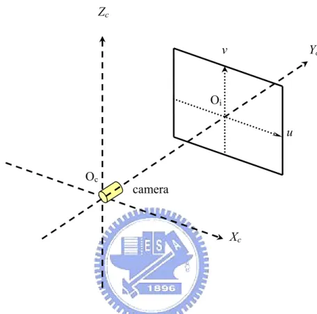
Fig. 2.1 The relationship of the camera and image coordinate systems... 7

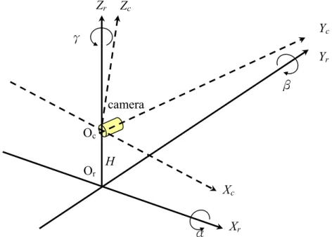
Fig. 2.2 The relationship of the camera and world coordinate systems. ... 8

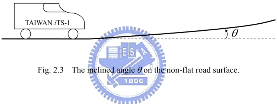
Fig. 2.3 The inclined angle θ on the non-flat road surface. ... 12

Fig. 2.4 The relationship of main and sub stereo cameras... 16

Fig. 2.5 The corresponding pixels between main and sub images... 21

Fig. 2.6 Calibration on both stereo cameras.. ... 24

Fig. 3.1 The flowchart of generic obstacle detection... 27

Fig. 3.2 The grayscale histogram of a road image with a blaze on the farther road surface... 30

Fig. 3.3 An example of the road image segmentation by different thresholds... 31

Fig. 3.4 An example of boundary detection... 33

Fig. 3.5 The flowchart of boundary detection... 34

Fig. 3.6 The flowchart of edge detection. ... 35

Fig. 3.7 The direction numbers for the 8-directional connecting process... 36

Fig. 3.8 Some restrictions on the boundary expansion ... 37

Fig. 3.9 The disjunctive point, p, satisfies φ <φ_th... 38

Fig. 3.10 The flowchart of boundary partition... 39

Fig. 3.11 The flowchart of the preprocessing. ... 40

Fig. 3.12 An example of the preprocessing.. ... 41

Fig. 3.13 The boundary gradient... 44

Fig. 3.14 The 1-D logarithmic search in the case of r = 4 (k = 2)... 48

Fig. 3.15 The bottom boundary and its corresponding top boundary. ... 51

Fig. 3.16 The flowchart of the discrimination process. ... 52

Fig. 3.17 The neighbor block of the boundary... 53

Fig. 3.18 The mean vector of the boundary. ... 54

Fig. 4.1 The flowchart of lane detection... 56

Fig. 4.2 The 3×3 mask for determining the gradients of the vertical edges... 60

Fig. 4.3 The constant marking width in the world coordinate system.. ... 61

Fig. 4.4 Steps of the marking detection. ... 63

Fig. 4.5 The possible ranges of the markings on both sides of the lane at the initial state. ... 64

Fig. 4.6 The image is divided into n zones, and the markings are detected from bottom to up... 65

Fig. 4.7 (a)~(f) are the intermediate phases where the zones are detected from bottom to up, respectively.... 66

Fig. 4.8 The flowchart of lane detection in the single mode... 69

Fig. 4.9 The flowchart of Decision Tree. ... 72

Fig. 5.1 Results of obstacle detection on a hill road. ... 76

Fig. 5.2 Results of obstacle and lane detection on the expressway... 77

Fig. 5.3 Results of obstacle and lane detection on the freeway... 77

Fig. 5.4 Results of lane detection on the straight roads. ... 78

Fig. 5.5 Results of lane detection on the crooked roads. ... 79

Fig. 5.6 Results of lane detection on the roads with shadows or the sunlight... 79

Fig. 5.7 Results of lane detection on the roads interfered with the text... 80

Fig. 5.8 Results of lane detection on the roads affected by the vehicles... 80

Fig. 5.9 Result of lane detection on the night road.. ... 81

Fig. 5.10 Result of lane detection on the rainy road.. ... 82

Fig. 5.11 Results of the real-time lane detection on the freeway of the sunny day... 84

Fig. 5.12 Results of the real-time lane detection on the freeway by night... 85

Fig. 5.13 TAIWAN iTS-1.. ... 86

Fig. 5.14 The GOLD system fails in the case of a non-flat road.. ... 87

List of Tables

Table 2-1 The effect on the distance by the variation in the camera height H... 14 Table 2-2 The effect on the distance by the variation in the inclined angle θ... 15 Table 3-1 The look-up table of predicting the vsg for every vmg. ... 50

Chapter 1 Introduction

1.1 Motivation

As the conveyances are getting growth with years, the traffic is becoming more and more serious in most developed countries. A lot of researches about the intelligent transportation systems (ITS), including the smart vehicles, the driving safety, and the traffic mobility, have been proposed in recent years. In fact, many problems are still expected to be overcome. Above all, one of the most interesting and important issues for the ITS applications is concerning the smart vehicles.

It is necessary to acquire the information about the on-road obstacles and the lane tendency while driving on the way. Thanks to the driver’s careless attitude, his/her moving vehicle may hit the obstacles on the road, or may deviate from the correct lane orientation, which induces the traffic accidents. Hence the on-vehicle obstacle and lane detection system plays a fundamental and essential role in moving vehicles. Such a system can either be the driver assistance function to warn the drivers of occurrences of which they may not be aware, or be the vision system of unmanned vehicles to supply the car controller with the road information for the goal of the automatic driving.

In general, the vision-based obstacle and lane detection system is a good choice for ITS applications. Cameras are mounted on the vehicle, and then the road images are captured and processed. The systems based on the vision have advantages of the high spatial resolution and the fast image scansion. Many approaches using the image processing have been developed [1], and different techniques will be reviewed in the next section.

1.2 Background

1.2.1 Related work of obstacle detection

The definition of obstacles induces the development of detection algorithms. Since the vehicles are most of obstacles on the road, some approaches to detect obstacles are limited to search for particular features and then to match them with specific patterns, such as the symmetry, textures, shapes, an approximate contour, and so on. In this case the processing can be focused on the analysis of a single still image. Broggi et al. perform a function of vehicle detection to locate and track the vehicle by exploiting the symmetry of the rear parts of a typical car and a bounding box satisfying specific aspect ratio constraints [2]. However, such a pattern-based approach may fail when characteristics of obstacles do not match the pre-defined model.

As we know, vehicles are not the only obstacles on the road. A generic obstacle is defined as an object rising out significantly from the road surface. Following this definition, the pattern-based approach does not work owing to the lack of a prior knowledge about generic obstacles on the road. More complex techniques must be imported to handle such a problem, and two and more images may need to be taken into account.

The optical flow-based approach utilizes a sequence of two or more images to obtain reliable and dense optical flows. In the assumption of the small difference between two successive images due to the short time interval, the two-dimensional motion between two images approximates the single direction. And therefore, the optical flow field can be computed and the ego-motion can be estimated. Giachetti et al. use a correlation technique to compute the flow field, and the obstacles moving with different speeds can be segmented by analyzing the velocity fields [3]. However, the optical flow-based approach may fail deriving from the lack of textures on the road, or from large displacements between two consecutive

frames due to the higher speed or vibrations of the vehicle.

Another technique similar to the optical flow-based approach is known as the motion-based method by estimating the motion of the ground plane and then detecting the obstacles whose motions differ from that of the ground [4-7]. In this method, it is necessary to make a tracking about the motion among images for large displacements, and as a consequence the assumption of rectilinear motions in optical flow-based methods is invalid. Since the scenes vary very much among images, it is difficult to identify the pixel correspondence. If the size of searching area is too small, the correct matching for the corresponding pixels may be missed. On the other hand, if the size is too large, too many possibilities may exist. Notice that both optical flow-based and motion-based approaches need expensive computational costs.

The stereo vision-based technique is also used to detect the generic obstacles. The GOLD system transforms both left and right stereo images into top views in order to remove the perspective effect. The ideal square obstacle is transformed into two triangles in the difference image of both remapped views. The polar histogram is constructed from the difference image and then the two peaks in the polar histogram are joined to identify the obstacle [2, 8].

Labayrade et al. also use both left and right stereo images to construct v-disparity image to detect potential obstacles whose disparities differ from that on the road surface. The angles between the cameras and the road are then estimated [9-10]. In conclusion the stereo vision-based method is a better framework than others, and is adopted in this thesis.

1.2.2 Related work of lane detection

It is the objective for lane detection to detect the relative position between the vehicle and the road, and to determine the lane information, such as the offset, the orientation, the curvature, and so forth. Since the structured roads are met in the practical applications, most researches focus on the analysis of marking roads where lane markings are painted on the road surface. Several features of the lane markings, including the constant lane width, the higher brightness on markings, the structured lane shape, etc.

The GOLD system removes the perspective effect by mapping the road image into the top view, and determines the lane markings by relying on the feature of the constant lane width, which may fail when the assumption of a flat road is not valid [8]. Based on the GOLD system, Jiang et al. model the lane as two straight lines to estimate the inclined angle on the condition of non-flat roads [11].

However, the road shape usually is not straight in real cases. Polynomials or splines may be better lane fittings than the straight line. Such a geometric model-based lane detection technique is more robust against the interferences such as shadows, textures, or other vehicles. Based on the lane geometry, the coefficients of lane model can be found out by several methods. LOIS, LANA, and RVP-I systems decide the coefficients with the maximum likelihood by completely searching the parameter spaces where all possibilities produced in the training phase are built [12-14].

Instead of searching throughout the databases, some road features are detected in the overall image in order to determine the coefficients. Yue Wang et al. [15] and Goldbeck et al. [16] use the edge-oriented methods to measure the matching degree between the model and the edge map in order to determine the parameters, respectively. Gonzalez et al. classify the objects in the image as the road surface, markings, or obstacles by a histogram-based segmentation method and then pixels belonging to the markings are taken into the fitting of

the lane model [17].

Different from the lane geometry, the statistical model can be used to specify the detection region of interest (ROI) in order to narrow the searching area [7, 18]. On the other hand, the ROI can also be determined according to the features of markings used in the TFALDA [19]. However, the statistical parameters and the weights of marking features have to be trained in advance.

Since the model-based approaches have more robust results and the use of the detection ROI can reduce the computational cost, both ideas are adopted in this thesis. The details will be proposed later.

1.3 Organization

This thesis is organized as follows. A review of algorithms about the obstacle and lane detections is given in this chapter. The preliminary knowledge of the computer vision is introduced in Chapter 2. In Chapter 3, the algorithm of the generic obstacle detection based on two top and bottom stereo cameras is developed. The approach to detect the lane is proposed in Chapter 4. And afterward the experimental results of both obstacle and lane detections are demonstrated in Chapter 5. Finally, a conclusion is presented in Chapter 6.

Chapter 2 Stereo Vision System

In this chapter the preliminary knowledge of the computer vision will be introduced. In the beginning, the relationship of image, camera, and world coordinate systems is discussed. And then the surface of the non-flat road is modeled. The architecture of two top and bottom stereo cameras and the calibration principle are presented finally.

2.1 Geometric Camera Model

2.1.1 Perspective projection

The scene points in the camera coordinate system can be captured by a camera and be projected onto the image pixels (u, v) in the image coordinate system, as illustrated in Fig. 2.1. This phenomenon can be described as the perspective projection, and the camera can be modeled quite well by the so-called ideal pinhole camera, which induces the projection equations as follows [20]:

(

Xc ,Yc ,Zc

)

c c u _Y X e u= (2-1) and c c v _Y Z e v= (2-2)

where (u, v) and are the image and camera coordinates, respectively. Note that

and are the intrinsic parameters of the camera, and are represented by

(

Xc ,Yc ,Zc

)

u e e _v : dv e du e_u = and _v = (2-3)

where du and dv are the physi

f f

cal width and height, respectively, of an image pixel. And f is the focal length of the camera.

image pixels of R2, and therefore, the homogeneous coordinate system is suitable for a general simple treatment of the perspective projection.

Fig. 2.1 The relationship of the camera and image coordinate systems.

Let is the 4×4 perspective transform matrix, expressed as follows: ⎡ = 1 0 0 0 0 0 0 1 0 0 0 0 0 0 v u proj e e P (2-4) tran u v Oi Yc Oc Zc Xc camera proj P ⎥ ⎥ ⎥ ⎦ ⎤ ⎢ ⎢ ⎢ ⎣ sforming Cv_h=

[

X_c Y_c Z_c 1

]

′ into Iv_h=

[

x_i y_i z_i 1

]

′, i.e. h proj h C Iv =P v (2-5)

where Cv_h and Iv_h are the homogeneous camera and image coordinates, respectively. Notice that the prime denotes the transpose.

i i y x u= (2-6) and i i y z v= . (2-7)

It is obvious that there exists the invertible matrix −1 satisfying

proj

P Cv_h= P_proj−1 Iv_h, and

however, there is no sufficient information from the image coordinates (u, v) of R2 to get the camera coordinates

(

X_c ,Y_c ,Z_c

)

of R3. The solutions about this issue will be presented later.

2.1.2 Point relationship of camera and world coordinates

In the following, it is necessary to perform positioning in three coordinate systems, Iv_h,

h

Cv , and Wv_h, shown in Fig. 2.1 and Fig. 2.2. The relationship of Iv_h and Cv_h, homogeneous image and camera coordinates, respectively, have been explained in Section 2.1.1. In this section the point relationship of Cv_h and Wv_h will be discussed, and the transformation from

h

Wv to Iv_h will be briefed in Section 2.1.3.

Zr Zc

Fig. 2.2 The relationship of the camera and world coordinate systems.

Yc Oc Xr camera Xc Yr Or H γ β α

The 4 × 1 vector Wv_h =

[

X_r Y_r Z_r 1

]

′ is the homogeneous world coordinates, associated with Cv_h by

T W

Cv_h= R_r v_h − v (2-8)

where R_r is the 4×4 rotation matrix between the camera and the road, and Tv is the 4×1 translation vector from Or to Oc, the origins of world and camera coordinate systems, respectively.

Often Tv is the 1-D translation from Or to Oc, expressed by:

[

]

′

= 0 0 H 0

Tv (2-9)

and H is the distance between Or and Oc.

In general, is however, composed of three 4×4 rotation matrices, , , and

, i.e. r R R_α R_β γ R γ β αR R R R_r = (2-10)

where α, β, and γ are the pitch, roll, and yaw angles counterclockwise looking at the origin Or from +Xr, +Yr, and +Zr axes, respectively, and

⎥ ⎥ ⎥ ⎦ ⎤ ⎢ ⎢ ⎢ ⎣ ⎡ − = 1 0 0 0 sin cos 0 0 cos sin 0 0 0 0 0 1 α αα α α R (2-11) ⎥ ⎥ ⎥ ⎦ ⎤ ⎢ ⎢ ⎢ ⎣ ⎡ − = 1 0 0 0 0 cos 0 sin0 1 0 0 0 sin 0 cos β β β β β R (2-12) ⎥ ⎥ ⎥ ⎦ ⎤ ⎢ ⎢ ⎢ ⎣ ⎡ − = 1 0 0 0 0 1 0 0 cos 0 0 sin sin 0 0 cos γ γγ γ γ R (2-13)

Usually the yaw angle, γ, can be taken no account without relating to the lane orientation on the road and can be withdrawn. Hence (2-10) can be replaced by:

(2-14) ⎥ ⎥ ⎥ ⎦ ⎢ ⎢ ⎢ ⎣ ⋅ ⋅ − ⋅ − ⋅ = = 1 0 0 0 0 cos cos sin sin

cos sin cos sin cos 0

sin β α α β α β α α β α β αR R R_r

and its inverse matrix is

(2-15) ⎥ ⎥ ⎥ ⎦ ⎤ ⎢ ⎢ ⎢ ⎣ ⎡ ⋅ ⋅ − ⋅ − ⋅ = = − 1 0 0

0 sin cos cos cos 0

sin0 cos sin 0

0 sin cos sin sin cos 1 β α β α β α α β α β α β α βR R R_r

(2-8) can be rewritten as:

(

C T

)

Wv_h = _r−1 v_h+v

R (2-16)

Substituting each term into (2-16) yields

(

Z H

)

Y X

X_r =cosβ⋅ _c+sinα⋅sinβ⋅ _c−cosα⋅sinβ⋅ _c+ , (2-17)

(

Z H

)

Y

Y_r = cosα⋅ _c+sinα⋅ _c + , (2-18) and Z_r =sinβ⋅X_c −sinα⋅cosβ⋅Y_c +cosα⋅cosβ⋅

(

Z_c+H

)

, (2-19) which transform a point from in the camera coordinates to in the world coordinates.

2.1.3 Point relationship of image and world coordinates

By the combination of (2-5) and (2-8), it yields

(

)

⎥ ⎥ ⎥ ⎦ ⎤ ⎢ ⎢ ⎢ ⎣ ⎡ − ⋅ ⋅ + ⋅ + ⋅ ⋅ − ⋅ ⋅ + ⋅ − ⋅ ⋅ ⋅ + ⋅ ⎥ ⎥ ⎥ ⎦ ⎤ ⎢ ⎢ ⎢ ⎣ ⎡ = − = = 1 cos cos sin sin cos cos sin cos sin sin sin cos 1 0 0 0 0 0 0 1 0 0 0 0 0 0 H Z Y X Z Y X Z X e e T W C I r r r r r r r r v u h r proj h proj h β α α β αα β α α β β β v v v v R P P (2-20)

The transformation from the point

(

X_r ,Y_r ,Z_r

)

in the world coordinates to the pixel (u, v) in the image coordinates can be described by

r r r r r u i i Z Y X Z X e y x u= = _α⋅ β_β⋅_{⋅ + α⋅ − α}+_⋅ β_β⋅_⋅ cos sin cos sin sin sin cos (2-21) and r r r r r r v i i Z Y X H Z Y X e y z v= = − α_α⋅_⋅ β_β⋅_⋅ +₊ α_α⋅_⋅ +_{− α}α_⋅⋅ _ββ_⋅⋅ − cos sin cos sin sin cos cos sin sin cos . (2-22)

If the roll angle, β, of the camera, approximates to zero, then

r r r u _{Y Z} X e u= _{α⋅ − α⋅} sin cos _(2-23) and r r r r v _{Y Z} H Z Y e v= α_α⋅_⋅ +_{− α}α_⋅⋅ − sin cos cos sin _{. (2-24)}

If α = 0 and β = 0, i.e. no rotation occurs between both coordinate systems, then (2-21) and (2-22) reduce to r r u _Y X e u = (2-25) and r r v _Y H Z e v= − . (2-26)

2.2 Modeling the Road Surface

2.2.1 Consideration for the angle of inclination on the non-flat road

Usually the surface on the real road is not flat, and it may be modeled as a succession composed of piecewise planes. For the simplification and the practicality, the road surface in this thesis is modeled as the plane with the inclined angle θ, formed by the road ground and the plane where the vehicle mounted the camera is standing, see Fig. 2.3.

TAIWAN iTS-1

θ

Fig. 2.3 The inclined angle θ on the non-flat road surface.

The (road) ground equation is stated as follows:

r r

r Y m Y

Z =tanθ ⋅ = _θ ⋅ , (2-27)

where m_θ =tanθ is the road inclination. Assume that both α and β approximate to zero, and combine (2-25), (2-26), and (2-27) to produce

u v v r e e v m e H u X ⋅ − ⋅ ⋅ = θ (2-28) v m e H e Y v v r = _{⋅ −} θ (2-29) v m e H m e Z v v r _{⋅ −} ⋅ = θ θ _{. (2-30)}

If the road inclination and the ground coordinates (u, v) in the image are given, the physical ground coordinates can be estimated by (2-28), (2-29), and (2-30).

θ

m

Notice that the intrinsic difference of the discussions between Section 2.1.3 and Section 2.2.1. Section 2.1.3 has proposed that a point in the world coordinate system can be projected onto the image plane, which is affected by the camera angles. It is never said that Z_r =0

means the road surface. Ideally, Z_r =0 may happen on the flat road. If the camera angles, i.e. α and β, are thought as what are included by the inclinations of the camera and the road, it can be true that Z_r =0 for certain α and β in every local zone is exactly the road plane, and the angles for Z_r =0 may be different zone by zone.

On the contrary, the inclined angle θ discussed in this section is a global consideration for the model of the non-flat road. It can be exactly said that (2-27) is representative of the road ground. Similarly, if the inclined angle θ is treated as what is included by the inclinations of the camera and the road, then the pitch angle α can never be considered. Furthermore, if β is small enough to be ignored, as assumed earlier, then three axes in the camera coordinates are coincided with those in the world coordinates.

2.2.2 Width mapping of image and world coordinates

In this section we focus on the mapping of the width on the road ground from the world coordinates to the image coordinates. From (2-28), it is easy to get

u v v r _e e v m e H u X ⋅ − ⋅ ⋅ ∆ = ∆ θ (2-31) and v u v r _e e H v m e X u=∆ ⋅ ⋅ − ⋅ ∆ θ _(2-32)

If the road inclination m_θ and ∆X_r, such as the lane width, are given, the pixel distance, say ∆u, of the abscissa in the image can be determined by (2-32).

2.2.3 Effects on distance accuracy associated with the inclined angle of the

road and the camera height

The distance of objects in front of the camera is a desire for the application of smart vehicles. As indicated in (2-29), the distance, , is associated with the camera height H and the inclined angle θ. However, H or θ may change due to the oscillation in motion or the non-flat road surface, which results in an inaccurate measure of distance. The effects on the distance by the camera height H and by the inclined angle θ will be discussed, respectively, and an ideal case is assumed that H = 135 cm and θ = 0°.

r

Y

¾ A: the variation in the camera height H

In this case θ is fixed and equals to zero. However, the change of results in the change of . From (2-29), a simple analysis can be to obtain the factor of variation H H H → +∆ r r r Y Y Y → +∆

(

∆Yr Yr

)

∆_H as follows: H H Y Y H r r ₌∆ ⎟⎟ ⎠ ⎞ ⎜⎜ ⎝ ⎛ ∆ ∆ (2-33)

It is obvious that

(

∆Y_r Y_r

)

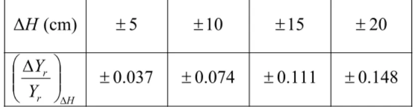
_∆H is only related to ∆H and is not affected by the distanceY_r. The change, ∆ , of the camera height due to the vibration in motion can be H

assumed to bound in ±20 cm. Table 2-1 shows some cases of different H∆ . For example, the maximum error of the distance on the condition of Y_r= 50 m and ∆ = 20 cm is 7.4 m. H

Table 2-1 The effect on the distance by the variation in the camera height H.

148 . 0 111 . 0 074 . 0 0.037 20 15 10 5 (cm) ∆ ± ± ± ± ⎟⎟ ⎠ ⎞ ⎜⎜ ⎝ ⎛ ∆ ± ± ± ± ∆H r r Y Y H

¾ B: the variation in the inclined angle θ

In this case H is fixed and equals to 135 cm. The error ∆Y_r derived from the change of θ

θ

θ → +∆ can also be computed by (2-29).

(

)

) 0 ( ° = ⋅ + − = ⋅ + − + − = − − ⋅ − ⋅ = − − ⋅ = ∆ ∆ ∆ ∆ + ∆ + ∆ + ∆ + θ θ θ θ θ θ θ θ θ θ θ θ θ θ Q r r r r r r v v v r v v r Y Y H m m Y Y H m m m m Y Y H m e m e H e Y v m e H e Y r r Y Y m H ₋ ⋅ ⋅ = ∆ 1 1 θ (2-34)

Furthermore, the factor of variation in θ is indicated by

1 1 − ⋅ = ⎟⎟ ⎠ ⎞ ⎜⎜ ⎝ ⎛ ∆ ∆ ∆ r r r Y m H Y Y θ θ (2-35)

It is clear that

(

∆Y_r Y_r

)

_∆θ is associated with not only ∆θ but also the distance . An observation reveals that the farther the distance is, the larger the absolute value of

r

Y

(

∆Yr Yr

)

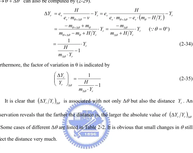
∆_θ is. Some cases of different ∆θare listed in Table 2-2. It is obvious that small changes in θstill affect the distance very much.

Table 2-2 The effect on the distance by the variation in the inclined angle θ.

(

∆Y_r Y_r

)

_∆θ ∆θ r Y (m) 1° 2° 3° -1° -2° -3° 10 0.148 0.349 0.635 -0.114 -0.205 -0.280 20 0.349 1.072 3.472 -0.205 -0.341 -0.437 30 0.634 3.465 -7.075 -0.280 -0.437 -0.538 40 1.071 -29.827 -2.809 -0.341 -0.509 -0.608 50 1.829 -4.409 -2.063 -0.392 -0.564 -0.659

According to the above discussions, a conclusion is given that ∆H can usually be ignored because the variation in θ has the dominant effect on the distance. Such a concept is used throughout this thesis.

2.3 Stereo Cameras

2.3.1 Relationship of main and sub stereo cameras

This thesis will propose the framework of both top and bottom stereo cameras, namely main and sub cameras, respectively, as illustrated in Fig. 2.4. The top camera is the main image sensor used for the obstacle and lane detection. The lower sub camera is the auxiliary utilized only to detect the obstacle.

Zr Zcm

Fig. 2.4 The relationship of main and sub stereo cameras.

Yr Ycs Ycm Main Camera Ocm Sub Camera Ocs Hm ΔH Hs

The relationship of homogeneous image, camera, and world coordinate systems, namely

hm

Iv , Cv_hm, and Wv_hm, respectively, of the main image sensor is the same as what is described in (2-5) and (2-8), that is,

hm proj hm C

Iv =P v (2-36)

and Cv_hm= R_rWv_hm−Tv_m (2-37)

where Tv_m=

[

0 0 H_m 0

]

′ is the 4×1 translation vector from Or to Ocm, the origin of the main camera coordinate system, and Hm is the distance between Or and Ocm.

The relationship of homogeneous main and sub coordinate systems is the combination of one translation and one rotation, which is expressed as follows:

[

hm m s

]

c

hs C T T

Cv = R v +v − v (2-38)

where is the 4×1 homogeneous sub camera coordinates, is the

4×4 homogeneous rotation matrix between main and sub cameras, and

[

′ = _{cs cs cs} 1 hs X Y Z Cv

]

R_c

[

]

′ = 0 0 s 0 s H Tv

is the 4×1 translation vector from Or to Ocs, the origin of the sub camera coordinate system. Notice that S m H H H = − ∆ (2-39)

is the distance between Ocm and Ocs.

Applying (2-36) through (2-38), the following equations are easily obtained

[

r h s

]

c hs W T Cv =R R v − v (2-40)

[

r h s

]

c proj hs proj hs C W T Iv =P v =P R R v − v (2-41) and _c−1 _proj−1 Iv_hs− _proj−1 Iv_hm=Tv_m−Tv_s

P P

2.3.2 Main camera coordinates from pixel correspondence of stereo images

Remember that Rc is the 4× homogeneous rotation matrix between main and sub 4 camera, as introduced in Section 2.3.1. Due to the pitch , roll, and yaw angles between main and sub cameras, is similar to (2-10). For the simplification and the convenience, is denoted by: c R Rc (2-43) ⎥ ⎥ ⎥ ⎦ ⎤ ⎢ ⎢ ⎢ ⎣ ⎡ = 1 0 0 0 0 0 0 22 21 20 12 11 10 02 01 00 r r r r r r r r r c R

and we know −1= . Thus (2-38) can be expanded as:

c R R′_c (2-44) ⎥ ⎥ ⎥ ⎦ ⎤ ⎢ ⎢ ⎢ ⎣ ⎡ ∆ + ⋅ + ⋅ + ⋅⋅ + ⋅ + ⋅ +∆ ∆ + ⋅ + ⋅ + ⋅ = ⎥ ⎥ ⎥ ⎦ ⎤ ⎢ ⎢ ⎢ ⎣ ⎡ ∆ + = ⎥ ⎥ ⎥ ⎦ ⎤ ⎢ ⎢ ⎢ ⎣ ⎡ 1 ) ( ) ( ) ( 1 1 20 21 22 12 11 10 02 01 00 H Z r Y r X r H Z r Y r X r H Z r Y r X r H Z Y X Z Y X cm cm cm cm cm cm cm cm cm cm cm cm c cs cs cs R

Furthermore, the following equations also hold true:

) ( ) ( 12 11 10 22 21 20 H Z r Y r X r H Z r Y r X r e Y Z e v cm cm cm cm cm cm v cs cs v s _{⋅ + ⋅ + ⋅ +∆} ∆ + ⋅ + ⋅ + ⋅ = = , (2-45) cm cm v m Y Z e v = , (2-46) and cm cm u m Y X e u = . (2-47)

The above three equations can be represented by the following linear algebraic system

(

)

⎥ ⎥ ⎦ ⎤ ⎢ ⎢ ⎣ ⎡− ⋅ − ⋅ ∆ = ⎥ ⎥ ⎦ ⎤ ⎢ ⎢ ⎣ ⎡ ⎥ ⎥ ⎦ ⎤ ⎢ ⎢ ⎣ ⎡ − − ⋅ − ⋅ ⋅ − ⋅ ⋅ − ⋅ 0 0 0 0 20 11 21 12 22 12 22 10 r v r e H Z Y X u e e v e r v r e r v r e r v r _{s v} cm cm cm m u v m v s v s v s (2-48)

By Cramer’s rule, the solution is given:

cm cm cm A X X det det = (2-49) cm cm cm A Y Y det det = (2-50) cm cm cm A Z Z det det = (2-51)

where

(

)

(

)

(

⎭ ⎬ ⎫ ⎩ ⎨ ⎧ ⋅ − ⋅ + ⋅ − ⋅ + ⋅ − ⋅ = _{s v v} u v v s m v s m u cm _e r v r e e e e r v r u e r v r v e A _{12 22 10 20 11 21} det

)

(2-52)

(

s v

)

v m cm u r v r e H e X =− ⋅ ₁₂⋅ − ₂₂⋅ ⋅∆ ⋅ det (2-53)

(

s v

)

v u cm r v r e H e e Y =− ₁₂⋅ − ₂₂⋅ ⋅∆ ⋅ ⋅ det (2-54)

(

s v

)

u m cm v r v r e H e Z =− ⋅ ₁₂⋅ − ₂₂⋅ ⋅∆ ⋅ det (2-55)

In summary it can be to obtain the main camera coordinates, Xcm, Ycm, and Zcm, on condition that the pixel correspondence of stereo image coordinates, um, vm, and vs, is given.

2.3.3 Pixel correspondence of stereo images

Multiplying both numerator and denominator of (2-45) by e_v Y_cm together, another form is indicated as:

) ( ) ( ) ( ) ( ) ( ) ( 12 11 10 22 21 20 12 11 10 22 21 20 12 11 10 22 21 20 cm v m v u v m cm v m v u v m v cm v cm cm v v u v cm cm u cm v cm cm v v u v cm cm u v cm cm cm cm cm cm v cs cs v s Y H e v r e r e e u r Y H e v r e r e e u r e Y H e Y Z e r e r e e Y X e r Y H e Y Z e r e r e e Y X e r e H Z r Y r X r H Z r Y r X r e Y Z e v ∆ + ⋅ + ⋅ + ⋅ ∆ + ⋅ + ⋅ + ⋅ = ∆ + ⋅ + ⋅ + ⋅ ⋅ ∆ + ⋅ + ⋅ + ⋅ ⋅ = ∆ + ⋅ + ⋅ + ⋅ ∆ + ⋅ + ⋅ + ⋅ = = (2-56)

In the same way, u_s is given

) ( ) ( 12 11 10 02 01 00 cm v m v u v m cm v m v u v m u s Y H e v r e r e e u r Y H e v r e r e e u r e u ∆ + ⋅ + ⋅ + ⋅ ∆ + ⋅ + ⋅ + ⋅ = (2-57)

Define two functions of three variables as follows:

n o e o e e m o o n m _{i v i} u v i i)≡ 0⋅ + 1⋅ + 2⋅ , , ( PreDot (2-58) n o e o e e m o o n m _{i v i} u v i i)≡ 0 ⋅ + 1 ⋅ + 2 ⋅ , , ( PostDot (2-59)

where is the inner product of PreDot(m,n,o_i)

[

o_i0 o_i1 o_i2

]

′ and _⎥ ⎦ ⎤ ⎢ ⎣ ⎡ n e e e m _v u v _. Let ci v i _Y H e v ≡ ∆ ∆ (2-60)

where the suffix i denotes the main or sub camera.

Hence (2-57) and (2-56) can be, respectively, described by:

m m m m m m u s v r r v u v r r v u e u ∆ ⋅ + ∆ ⋅ + = 12 1 02 0 ) , , ( PreDot ) , , ( PreDot (2-61) m m m m m m v s v r r v u v r r v u e v ∆ ⋅ + ∆ ⋅ + = 12 1 22 2 ) , , ( PreDot ) , , ( PreDot . (2-62)

From the similar process, um and vm can be obtained as follows:

) , , ( PostDot ) , , ( PostDot 1 0 r u v r u v e u s s s s u m = (2-63) ) , , ( PostDot ) , , ( PostDot 1 2 r u v v r u v e v s s s s s v m ∆ − = (2-64) where ∆v_s =

{

e_v⋅∆v_m

} {

PreDot(u_m,v_m,r₁)+r₁₂⋅∆v_m

}

(2-65) ¾ Part A: the condition of Zr = 0

The relationship of Zr and the main camera coordinates can be found in (2-19):

(

cm m

)

cm cm

r X Y Z H

Z =sinβ⋅ −sinα⋅cosβ⋅ +cosα⋅cosβ⋅ + (2-66) Instead of (2-66), (2-67) results from the fact of Zr = 0 on the ground.

(

cmg m

)

cmg

cmg Y Z H

X − ⋅ ⋅ + ⋅ ⋅ +

⋅

=sinβ sinα cosβ cosα cosβ

0 (2-67)

where the suffix g indicates the ground of Zr = 0.

By algebraic manipulations, ∆v_mg can be determined, that is,

[

]

⎭ ⎬ ⎫ ⎩ ⎨ ⎧ + ⋅ − + ⋅ ⎥⎦ ⎤ ⎢⎣ ⎡ ∆ − = ∆ = ∆ _{v mg} u v mg m cmg v mg _e e v e u H H Y H e v α α β tan cos tan (2-68)

To summarize, it is able to determine the sub image coordinates, usg, and vsg, of the ground from (2-61) and (2-62) on condition that umg, vmg, and ∆v_mg are known.

¾ Part B: the condition of the same Yr

Given the pixel correspondence between both stereo images, i.e. in the main image associated with in the sub image, as illustrated in Fig. 2.5, if there exists with as same as that of , the goal is to find out its corresponding in the sub image.

) , ( P_m1 u_m1 v_m1 ) , ( P_s1 u_s1 v_s1 ) , ( P_m2 u_m2 v_m2 Y_r P_m1 ) , ( P_s2 u_s2 v_s2

Applying (2-18) to the equality of Y_r at P_m1 and P_m2 yields

(

cm m

)

cm

(

cm m

)

cm Z H Y Z H

Y + ⋅ + = ⋅ + ⋅ +

⋅ ₁ sin ₁ cos ₂ sin ₂

cosα α α α (2-69) and (2-69) implies 1 1 2 2 1 tan tan 1 cm m v m v cm e v Y v e Y + ⋅ ⋅ ⋅ + = α α (2-70)

By the definition of ∆v_m in (2-60), it yields

1 1 2 2 _tan tan m m v m v m _{e v} v v e v ⋅∆ ⋅ + ⋅ + = ∆ α α (2-71)

Since is known from the pixel correspondence of and , can be derived from (2-61) and (2-62) by using (2-71) to get

1 m v ∆ P_m1 P_s1 P_s2 ( u_s2 ,v_s2) 2 m v ∆ .

Fig. 2.5 The corresponding pixels between main and sub images. Pm2 (um2, vm2)

Pm1 (um1, vm1)

Main Image Sub Image

Ps2 (us2, vs2)

In this case, the target is to determine associated with

whose is the same as that of .

) , ( P_s2 u_s2 v_s2 P_m2( u_m2 ,v_m2) r X P_m1( u_m1 ,v_m1)

In the beginning, R_r in (2-14) is re-presented by

(2-72) ⎥ ⎥ ⎥ ⎦ ⎤ ⎢ ⎢ ⎢ ⎣ ⎡ = 1 0 0 0 0 R R R 0 R R R 0 R R R 22 21 20 12 11 10 02 01 00 r R

and it is obvious that −1 = . And then (2-17) becomes

r R R′_r

(

Z H

)

Y X X_r =R₀₀⋅ _c+R₁₀⋅ _c+R₂₀⋅ _c+ (2-73) Applying (2-73) to the equality of X_r yields

2 20 2 10 2 00 1 20 1 10 1 00 R R R R R R ⋅X_cm + ⋅Y_cm + ⋅Z_cm = ⋅X_cm + ⋅Y_cm + ⋅Z_cm (2-74) Let E_i =R₀₀⋅X_cmi +R₁₀⋅Y_cmi+R₂₀⋅Z_cmi

⎭ ⎬ ⎫ ⎩ ⎨ ⎧ ⋅ + ⋅ + ⋅ ⋅ ∆ ∆ = ⎭ ⎬ ⎫ ⎩ ⎨ ⎧ ⋅ + ⋅ + ⋅ ⋅ = mi v u v mi mi cmi cmi v v u v cmi cmi u v cmi v e e e u v H Y Z e e e e Y X e e Y 20 10 00 20 10 00 R R R R R R

(

, ,R0 PostDot _{mi mi} mi v u vH ⋅ ∆ ∆ =

)

(2-75)

Substituting (2-75) into (2-74) yields

(

)

(

)

1 0 1 1 0 2 2 2 _{PostDot , ,R} R , , PostDot m m m m m m _{u v} v v u v = ∆ ∆ (2-76)

Since is given from the pixel correspondence of and , can be determined from (2-61) and (2-62) by using (2-76) to get

1 m v ∆ P_m1 P_s1 P_s2 ( u_s2 ,v_s2) 2 m v ∆ .

2.4 Calibration Principles

2.4.1 Calibration on both stereo cameras

The calibration on stereo cameras is a very important issue. The goal is to determine the relationship between both stereo cameras, and the result influences the accuracy of 3-D reconstruction. Once the calibration is finished, it is reasonable to suppose that the relative position between both cameras is invariant in use.

For the application in this thesis, we wish that no rotation occurs between both cameras to avoid the matrix calculation for the real-time consideration. However, it is difficult to reduce to zero in whole for the pitch, roll, and yaw angles between both cameras. But it is sure that we do our best to minimize the angles as small as possible.

The idea of the calibration is to transform both images into the same coordinate domain, and then to match the same objects in both images with each other. The ground on the road is an ideal choice for the pattern matching. As mentioned in Section 2.3.3, the transformation from the sub image coordinate system into the main image coordinate system is called “Vision Transform.” The road image is transformed from the sub image domain into the main image domain, and the ground in both images is coincided with each other after the calibration.

Steps for the calibration on both stereo cameras are as follows:

(1) Set up the main camera to satisfy that its optical axis is paralleling the ground, i.e. α = 0 and β = 0.

(2) Set up and regulate the sub camera by using Vision Transform to match the texture on the ground as possible, as displayed in Fig. 2.6.

(3) After setting up both cameras, estimate the angles by completely matching the ground texture, and then the relationship between both cameras is determined.

Fig. 2.6 Calibration on both stereo cameras. (a) The main (top) image. (b) The sub (bottom) image. (c) The sub image in (b) is mapped into the main image domain by Vision Transform. (d) The difference between (a) and (c).

(b)

(c)

2.4.2 Calibration on the main camera and the road

Due to the vibration in motion or the non-flat road surface, the pitch and roll angles, α and β, between the main camera and the road are always different. As discussed in Section 2.2.1, there exist certain α and β in every local zone so that Z_r =0 is exactly the road plane. Here α and β for every local zone of Z_r =0 are interesting.

Arrange (2-68) in another form:

( )

(

) {

v u v mg cmg v m mg e e e u Y e H v + − ⋅ ⎭ ⎬ ⎫ ⎩ ⎨ ⎧ ⋅ ⎟ ⎠ ⎞ ⎜ ⎝ ⎛ + ⎪⎭ ⎪ ⎬ ⎫ ⎪⎩ ⎪ ⎨ ⎧ ⋅ = − α α β tan cos tan

_}

(2-77)

If some data of u_mg, v_mg, and Y_cmg are given, then the unknowns,

( )

H_m ,

(

tanβ cosα

)

, and

(

−tanα

)

, of (2-77) can be solved by the least-squares method. However, as proposed in Section 2.2.3, the camera height has a smaller effect on the distance accuracy than the angles, and accordingly, can be taken as a constant and be moved to the left side of (2-77). Again, (2-77) becomes m H

(

) {

v u v mg cmg m v mg e e e u Y H e v + − ⋅ ⎭ ⎬ ⎫ ⎩ ⎨ ⎧ ⋅ ⎟ ⎠ ⎞ ⎜ ⎝ ⎛ = ⎪⎭ ⎪ ⎬ ⎫ ⎪⎩ ⎪ ⎨ ⎧ + − α α β tan cos tan

_}

(2-78)

and two unknowns,

(

tanβ cosα

)

and

(

−tanα

)

can be solved according to the same way. Finally, both α and β can be determined by the coefficients of (2-78).

Chapter 3 Generic Obstacle Detection

Since the preliminary knowledge of the computer vision has been proposed in Chapter 2, the algorithm of generic obstacle detection based on both stereo cameras will be introduced in this chapter. Two cameras are mounted top and bottom on the vehicle, and the top and bottom images captured by them are called the main and sub images respectively. Most manipulations are performed in the main image, and the sub image is used in the pattern matching. The details will be presented in the following.

3.1 Overview

Fig. 3.1 shows the flowchart of generic obstacle detection. The dashed blocks mean the successive detection mode and are not performed in the initial frame. In the beginning, the procedure of the preprocessing is executed in order to simplify the following detection. In the preprocessing, the road image captured by the main camera is segmented according to the gray levels and the so-called Minimum Ground in the main image is defined, which will be introduced in Section 3.4.

Proceeding to the next process, the flow enters the principal detection loop. In this detection loop, the boundaries are determined one by one, and then they are discriminated between the ground and obstacle boundaries. The so-called obstacle boundaries are the interconnecting boundaries between the ground and obstacles, and the others are called the ground boundaries. The discrimination method will be presented in Section 3.6.

The similar detection process is repeated until the Row Leader arrives at its ending. After that, all obstacle boundaries have been determined and then are updated for the detection in the next frame. The obstacle boundaries are divided into the motion and roadside boundaries according to their slopes. The boundaries with the sharp slopes are classified into the roadside

ones, and the others are the motion ones. And then the roadside boundaries are fitted to only the left and right roadside boundaries which can roughly bound the roadsides on the left and right sides of the lane.

If the obstacles have been detected in the last frame, they will be tracked in the current frame before the regular detection loop. However, only the motion boundaries can be tracked. The obstacle tracking can stabilize the detection result and reduce the detection time. The details will be proposed in Section 3.7.

START

Preprocessing

Fig. 3.1 The flowchart of generic obstacle detection.

Boundary Detection

Discrimination of Obstacle and Ground

Boundaries Tracking End of Row Leader? frame ← frame + 1 Updating

3.2 Image Segmentation by Thresholding

In this section the goal is to segment the road image into several groups according to the gray levels. Given a grayscale image, the mean and variance within the region of interest (ROI) in the grayscale histogram h_l, l∈

[

0,255

]

, are respectively computed as:

[ ] 0 1 0 , M M M l h H L l l = ⋅ = ∈

∑

µ (3-1)

(

)

[ ] 2 0 1 0 2 0 2 , 2 ⎟⎟ ⎠ ⎞ ⎜⎜ ⎝ ⎛ − = − ⋅ = ∈

∑

M M M M M l h H L l l µ σ (3-2)

where is the gray level, L and H are, respectively, the low and high bounds of the ROI, and , , and are, respectively, the zero, first, and second moments of the histogram to the origin, represented as follows:

l 0 M M₁ M₂ [ ]

∑

∈ = H L l l h M , 0 (3-3) [ ]

∑

∈ ⋅ = H L l l l h M , 1 (3-4) (3-5) [

∑

] ∈ ⋅ = H L l l l h M , 2 2

The number of clusters in the ROI is not unique if and there exists a threshold partitioning the region into two clusters so as to maximize the between-class variance, say

, where 2 2 th σ σ > th l 2 2 , 1 B σ

(

)

2 2 1 2 1 2 2 , 1 ωω µ µ σ_B = − (3-6) 0 1 0 1=M M ω (3-7) 1 2 1 ω ω = − (3-8) 1 0 1 1 1 M M = µ (3-9)

(

)

(

1

)

0 0 1 1 1 2 M M M M − − = µ (3-10)

(the zero moment of histogram within class 1 to the origin) (3-11) [ )

∑

∈ = th l L l l h M , 1 0

and (the first moment of histogram within class 1 to the origin) (3-12)

[ )

∑

∈ ⋅ = th l L l l l h M , 1 1

The above clustering process can be applied to each cluster iteratively until 2 2 or

th σ σ ≤ [ ] th l hl P M

∑

_{∈ 255} ≤ , 0

0 . The reason to bound the population within the ROI in the grayscale histogram is that the small class may be useless and be referred to the noise as detecting the obstacle in the road image. Therefore it is a benefit for the following processing to avoid the small cluster.

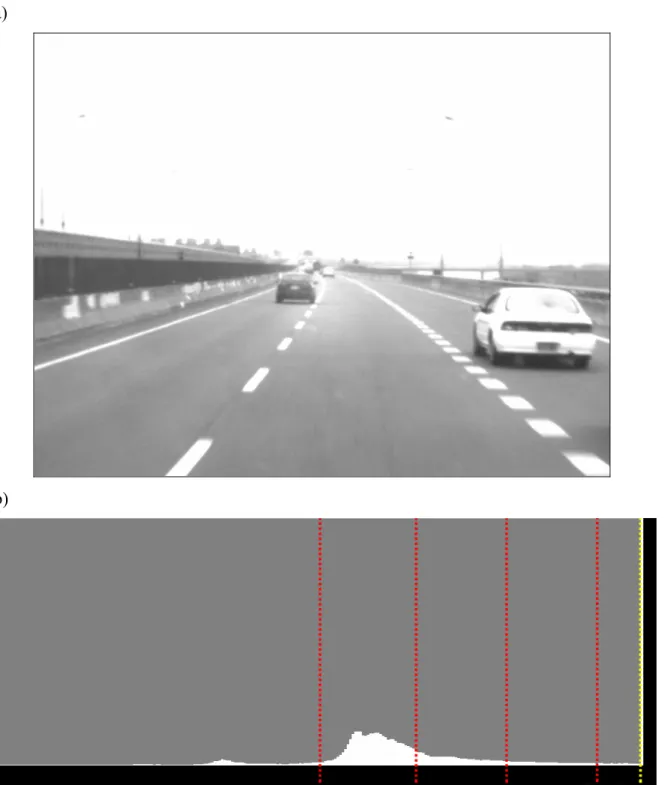
On condition of a blaze of daylight or the illimitable highway the gray levels on the farther surface of the road are similar to those in the heavens, and hence both may be the same class after the clustering process. As the histogram in Fig. 3.2 (b), the farther surface and the sky are classified the same by the gray level, say . However, there exists a threshold, namely , meeting that , used to replace for the separation

between the road and the sky if > . An example is demonstrated in Fig. 3.3. max l bright l _{l l} h_l P_bright bright ≥

∑

255= lmax bright l l_max

Fig. 3.2 The grayscale histogram of a road image with a blaze on the farther road surface. (a) A road image with a blaze on the farther road surface. (b) The grayscale histogram of (a).

(a)

(b)

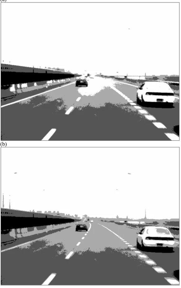
Fig. 3.3 An example of the road image segmentation by different thresholds. (a) The segmented image of Fig. 3.2 (a) by the threshold . (b) The segmented image of Fig. 3.2 (a) by the threshold .

max

l bright

3.3 Boundary Detection

The goal of boundary detection is to determine the significant boundaries which could be the textures on the ground, the interconnection between the ground and obstacles, or the edges on the obstacles. Since the road image has been segmented as described in Section 3.2, the boundary is the connection of edge pixels between two different clusters. An example is displayed in Fig. 3.4. The detection process will be proposed later.

3.3.1 Overview

Since the boundary is composed of edge pixels between two different clusters, the idea of boundary detection is to determine an edge pixel at first, and then to expand it into a boundary, as illustrated in Fig. 3.4.

In practice, a boundary is represented as the set of rows in the road image, and only one row per boundary column has to be recorded. Therefore, the size of each boundary can be simply regarded as the number of boundary columns. The target here is to determine the corresponding rows for each boundary column.

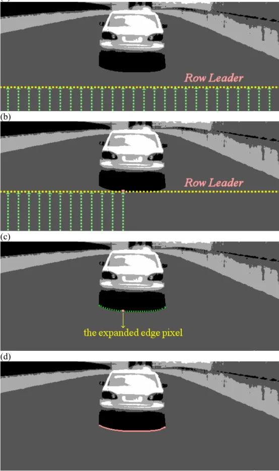
In order to detect the edge pixel for the expansion, pixels are scanned row by row for every column. As shown in Fig. 3.4 (a), the row bound, namely the Row Leader, is to limit what the current row can not exceed while scanning the edge, which guarantees that the edge pixel with the lowest row among all columns is found out first. And the lowest boundary is then produced by expanding the lowest edge pixel. Consequently, all boundaries will be detected in order from bottom to top in the segmented image.

The flowchart of boundary detection is shown in Fig. 3.5. If an edge pixel is found out at a certain column, the boundary is confirmed after the expansion process. A boundary is valid if its size is large enough, and it will be partitioned into several ones according to its disjunctive points, which will be introduced later.

(a)

(b)

(c)

(d)

Fig. 3.4 An example of boundary detection. (a) The current row can not exceed the Row Leader while scanning the edge. (b) The edge pixel of the lowest row is detected first. (c) The

then a new iteration is run. This process is repeated until any valid boundary is found out or the Row Leader arrives at its ending.

START Edge Detection Edged ? Boundary Expansion Valid ? Boundary Partition column ← column+1 End of column ? column←beginning column Boundary Detected ? End of Row Leader? Move up the Row Leader END

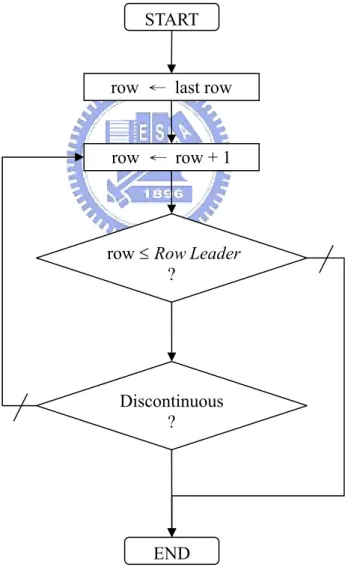
3.3.2 Edge Detection

As mentioned above, an edge is mode up of two different clusters in the segmented image. And an edge pixel is defined as the upper one of two pixels with different clusters. The edge detection is to determine an edge row for a given column on condition of

. The edge row corresponding to the given column is searched from the row of the last iteration to the Row Leader, and this process is terminated when an edge pixel

is found out. Fig. 3.6 shows the flowchart of edge detection.

Leader Row

row≤

START

Fig. 3.6 The flowchart of edge detection. END Leader Row row≤ ? Discontinuous ? row ← row + 1 row ← last row

3.3.3 Boundary Expansion

Given an edge pixel, the boundary can be leftward and rightward extended according to the same cluster. An 8-directional connecting process is used to extend the boundary. Fig. 3.7 indicates the direction numbers. Since the expanded edge pixel is the upper one whose cluster differs from that of the lower one, its direction number can be initialized to 0. And then the boundary is extended leftward and rightward by searching for the ways clockwise and counterclockwise, respectively. 4 5 3 6 2 7 1 0

Fig. 3.7 The direction numbers for the 8-directional connecting process.

The expansion process stops on some conditions stated as follows: (1) The current searching pixel comes back to the beginning entry.

(2) A U-turn is too deeper because two similar boundaries are closer very much. Fig. 3.8 (a) displays such an example.

(3) There are too many steps of the vertical motion at a time. It could be the case of the vertical boundary on the obstacles, which is not desired, as shown in Fig. 3.8 (b).

Finally, it is necessary to notice that only the lowest rows for every columns of the boundary have to be recorded.

Too many vertical steps A deeper

U-turn

(b) Too many vertical steps (a) A deeper U-turn

Fig. 3.8 Some restrictions on the boundary expansion. (a) A deeper U-turn. (b) Too many vertical steps.