Development of a feedforward active noise control system by using the H-2 and H infinity model matching principle

DEVELOPMENT OF A FEEDFORWARD ACTIVE

NOISE CONTROL SYSTEM BY USING THE H

AND H

MODEL MATCHING PRINCIPLE

M.-R. B  H.-P. C

Department of Mechanical Engineering, Chiao-Tung University, Hsin-Chu 30050, Taiwan, Republic of China

(Received 4 April 1995, and in final form 3 September 1996)

Two novel active noise control techniques on the basis of feedforward H2and Haoptimal

model matching principle are proposed. These methods effectively overcome the problem of unstable inverse plant resulting from the inherent non-minimum phase property of the cancellation path. The proposed algorithms are implemented by using a digital signal processor. The experimental results obtained by using H2and Hafeedforward techniques

show attenuation for stationary noise in a duct as comparable to those of conventional methods. The proposed methods also have potential in suppressing transient noises that have been the major difficulty in adaptive methods. Comparisons of the methods are summarized.

7 1997 Academic Press Limited

1. INTRODUCTION

Persistent research interest has developed in the area of active noise control (ANC) since Lueg filed his patent in 1936 [1]. ANC serves as a promising alternative to conventional passive control methods, because it provides advantages such as improved low frequency performance, reduction of size and weight, zero back pressure, reduction of energy consumption and programmable flexibility of design [2]. A vast amount of literature has been produced in the past and a very good review can be found in references [3, 4]. In the ANC configurations to date, feedforward control has become the most widely used technique (whenever the upstream reference signal is available) because it provides wider control bandwidth within moderate controller gain than feedback control [4]. Two representative feedforward ANC approaches are Roure’s method [6] and the filtered-x least mean square (FXLMS) method and their variants [7–9]. The former is based on a fixed controller, while the latter is based on an adaptive controller.

The main objective of this study is to propose two ANC techniques by using the feedforward H2and Hamodel matching principle. These methods are compared with the

conventional fixed and adaptive methods through intensive experiments involving various synthetic and practical noise types. These methods effectively overcome the problem of the unstable inverse plant resulting from the inherent non-minimum phase (NMP) property of the cancellation path. The NMP behavior is a fundamental issue which is at the heart of control system design, but is often an overlooked factor that could seriously degrade the ANC performance in attenuating broadband random noises. In the H2 and Ha

methods, the NMP problem is handled in optimal ways, depending on the criteria. In the 0022–460X/97/120189 + 16 $25.00/0/sv960765 _{7 1997 Academic Press Limited}

derivation, it is also insightful to see how the NMP property imposes a constraint on the achievable performance.

The algorithms were implemented by using a floating point digital signal processor (DSP). Experiments were performed on a duct of finite length to justify the proposed methods. The experimental results obtained by using the H2 and Ha feedforward

techniques show attenuation for stationary noises comparable to those of conventional methods. The proposed methods also have potential in suppressing transient noises, which have been the major cause of difficulty in the adaptive methods. However, the proposed methods are not intended to be substitutes for the prevailing methods such as the FXLMS algorithm that achieve as much as 50 dB of periodic noise attenuation. As pointed out by a reviewer, fixed and adaptive controllers each have their own properties and uses. For stationary noise or narrow-band noise, the FXLMS method is still a powerful one in terms of performance and robustness. For non-stationary, broadband or transient noises, the H2

and Ha feedforward techniques serve as useful alternatives.

This paper is organized as follows. Firstly, the nature and importance of the NMP problem will be addressed. Then, ANC algorithms based on H2 and Ha optimization

criteria will be presented. In the next section, the techniques developed are validated by experimental investigations and the methods are compared. In the final section, conclusions are presented.

2. THEORY AND METHODS

In what follows, the formulations are expressed in terms of sampled data systems and a discrete time base to facilitate the presentation and the digital implementation of the ANC algorithms. A plant is said to be NMP if its transfer function G(z) contains a pure time delay (z−N_{, N}q 0) and/or unstable zeros outside the open unit disk (=z= e 1). The

immediate difficulty that one will have with the NMP property is that the inverse plant is not implementable because G(z)−1 _{will be non-causal if G(z) contains a pure time}

delay and unstable if G(z) contains unstable zeros. Apart from the above facts, an NMP plant is characterized as being malign for control system design because it also has some undesirable properties: e.g., a sluggish response, undershoot or a non-unique magnitude–phase relationship [11, 12]. Control methods could break down in the face of the NMP behavior, so that designers traditionally strive to avoid it whenever possible. Although these NMP behaviors used to be related to feedback control, they still impose design constraints on feedforward controllers, as will become clear later.

It may appear that the NMP problem is only an anomalous case in physical systems. Unfortunately, there are many application domains, such as the control of flexible structures and acoustic fields, in which the NMP problem is rather common. More precisely, the NMP problem is almost certain to arise in the cases of non-colocated control: i.e., the sensor and the actuator are not loaded at the same point. In-depth discussions of the NMP property and non-colocated control can be found in references [13, 14].

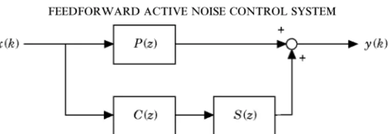
What is the implication of the NMP problem in the context of ANC problems? This will become clear if one poses the feedforward ANC problem of a duct into a model matching problem, as shown in Figure 1. The sampled signal x(k) is the input disturbance noise. P(z) is the transfer function of the primary acoustic plant, where z denotes the

z-transform variable. S(z) is the transfer function of the cancellation path formed by the actuator, the acoustic error path and the sensor. Hence, the ANC problem amounts to

Figure 1. A system block diagram of the feedforward ANC problem. P(z), S(z) and C(z) are the discrete-time transfer functions of the primary acoustic path, the secondary path and the controller, respectively.

finding the controller C(z) such that the residual field y(k) can be minimized. In order to match the characteristics of the paths P(z) and C(z)S(z), one is tempted to set

C(z) = −P(z)/S(z). (1)

In fact, this is essentially the central idea of Roure’s approach [5], which will certainly work well for a minimum phase plant S(z). However, it frequently occurs that S(z) is NMP, so that direct application of equation (1) will give a non-implementable controller. If the unstable controller of equation (1) is employed, unstable pole-zero cancellation will occur in the cancellation path and give disastrous results. This is the previously mentioned design constraint imposed on feedforward controllers, which is similar to the interpolation

constraintsof feedback control [12]. Truncating the non-causal part of C(z) that generally arises in frequency domain analysis, as suggested by Roure, will not completely eliminate the difficulty. The fact that effective attenuation can be obtained only in the cases of MP plants can also be arrived at by a Wiener filtering type of argument [15]. However, researchers in the area of digital signal processing tend to pay more attention to the causality problem, which is in fact a special case of the aforementioned NMP problem. In any rate, it is highly desirable to develop an ANC method that would effectively match the primary path and the cancellation path with respect to some optimal criteria when the NMP behavior is an issue. Elegant solutions to this problem are available in robust control theory. Two model matching algorithms capable of dealing with NMP problems in ANC applications are proposed in this paper.

The first approach is based on H2 optimization. Recall that the feedforward ANC

problem is equivalent to matching the characteristics of the primary path and the cancellation path. The degree of match can be measured on various criteria. The criterion employed in the following method is the 2-norm in Hilbert space. One defines the squared error o2

2 as

o2

2=>P(z) + C(z)S(z)>22, (2)

where the 2-norm of a scalar transfer function is defined as >G(z)>2,

0

g

Then, the feedforward model matching problem reduces to the following: find a biproper and stable transfer function C(z) to minimizeo2

2. The key to undo the difficulty caused by

the NMP problem is inner–outer factorization. It can be shown that every proper and stable function T(z) has a factorization [16]

T(z) = Ta(z)Tm(z), (4)

with Ta(z) being an all-pass function and Tm(z) being a minimum phase function.

S(z) = Va(z)Vm(z). Substitute the factored form into equation (2) and omit (z) for

simplicity. Hence, one has o2

2=>P + VaVmC>22=>VaV−1a P+ VaVmC>22

=>Va(V−1a P+ VmC)>22=>V−1a P+ VmC>22. (5)

In the last step, the fact Vahas a bounded constant magnitude on the unit circle has been

used. Note that, in Hilbert space, V−1

a P can be uniquely decomposed into a stable part

and an unstable part (by partial fraction expansion) as

V−1

a P= (V−1a P)u+ (V−1a P)s, (6)

where (V−1

a P)uand (V−1a P)scorrespond to the unstable and stable parts, respectively. Note

that these two terms belong to subspaces that are orthogonal complements to each other. Then, equation (5) can be further written as

o2 2=>(V −1 a P)u+ (V−1a P)s+ VmC>22=>(V −1 a P)u>22+>(V −1 a P)s+ VmC>22. (7)

The Pythagoras theorem in Hilbert space was used in the last equality [12]. It is now clear that the unique optimal Copt(z) is

Copt(z) = −V−1m (V−1a P)s (8)

and the minimum of o2

2 equals >(V−1a P)u>22. Note that this minimum value dictates

the ultimately achievable performance imposed by the NMP constraint, which is similar to the situations in feedback control. Ideally, this value will be zero if the system is MP.

Another elegant approach to match the characteristics of the primary path and the cancellation path is based on the Ha optimization. Thea-norm of a scalar transfer

function G(z) is defined as

>G(z)>a= sup u$[ − p,p]=G(e

ju_{)=, (9)}

where ‘‘sup’’ denotes the least upper bound. Similarly as in the H2-norm optimization, the

feedforward ANC problem can be recast into the following problem: find a biproper and stable transfer function C(z) to minimize the a-norm error

oa=>P + SC>a. (10)

In addition to the mathematical sense of model matching, the a-norm optimization provides nice physical insights into the ANC problem. It can be proved that [12]

>P + SC>a= sup x(k)

>y(k)>2

>x(k)>2

, (11)

where x(k) and y(k) denote the input noise and the residual noise at the output, respectively (see Figure 1). The 2-norm of the sampled input and the output signals x(k) and y(k) is defined as

>· >2=

$

%

Thus, minimizing the a-norm of the transfer function is tantamount to minimizing the maximum value of the input-output energy ratio (measured by the 2-norm).

Again similarly as in the 2-norm model matching problem, the problem can now be formulated in terms of the a-norm as

min>P + SC>a= min>P + VaVmC>a= min>VaV−1a P+ VaVmC>a

=>min>Va(V−1a P+ VmC)>a= min>V−1a P+ VmC>aetc, (13)

where the inner–outer expansion of the transfer function S(z) and the property of the all-pass function =Va(eju)= = 1, u $(−p, p] have been used.

Next, define R = V− 1

a Pand Q = −VmC. The problem in equation (13) then reduces to

the following: find a stable and proper Q(z) for a given proper (not necessarily stable) R(z) such that >R − Q>a is minimized. This is the well-known Nahari problem and the

minimum value can be shown to be the Hankel norm of the operator R [17, 18]. This result can be interpreted as saying that the shortest distance from a given unstable system to the nearest stable one equals the Hankel norm of the unstable one: i.e., the Hankel norm is a measure of instability.

There are two methods available for solving the Nahari problem: the Nevanlinna–Pick interpolation method [12] and the state space method [16]. The latter method is employed in this paper, since it is numerically more reliable than the other. To keep the presentation to a reasonable length, the procedure of finding the optimal transfer functions Q(z) or C(z) is summarized in the following algorithm. For the underlying theory, consult reference [16]. In this algorithm the packed matrix notation is used to denote the state space realization: i.e.,

x(k + 1) = Ax(k) + Bu(k), y(k) = Cx(k) + Du(k), is denoted as [A, B, C, D].

Step. 1. Find the inner–outer factorization of the cancellation path: S(z) = Va(z)Vm(z)

with both Vm(z) and V−1m (z) being proper and stable.

Step. 2. Find a minimal realization of R(z) and separate it into the stable part and the unstable part R(z) = [A, B, C, 0] + (stable part).

Step. 3. Solve the discrete-time Lyapunov equations for the controllability grammian Lc

and the observability grammian L0:

Lc− ALcAT= BBT, L0− ATL0A= CTC. Step. 4. Find the maximum eigenvalue l2 _{of L}

cL0 and a corresponding eigenvector w. Step. 5. Define f(z) = [A, w, C, 0], g(z) = [−AT_,l− 1_L

ow, BT, 0]. Step. 6. Set Qopt(z) = R(z) −lf(z)/g(z).

Step. 7. Calculate the optimal controller Copt(z) = −Vm− 1(z)Qopt(z).

A caution about the Hamodel matching method is in order. Unlike the H2method, the Ha method per se is to achieve model matching in an optimal way subject to the worst case input [12]. The optimization of the Ha method is carried out for the whole class of

input with bounded energy. With some manipulations, it can be shown that sup x(k) >y(k)>2 >x(k)>2E supx(k) >z(k)>2 >x(k)>2 , (14)

where z(k) denotes the output signal without the feedforward control, as shown in Figure 1. This inequality merely states that the least upper bound of the ratio between the controlled output and the input is not greater than that of the ratio between the uncontrolled output and the input for every possible input with bounded energy. However, it may be possible to find some special cases in which the 2-norm of the controlled output is greater than the uncontrolled output, although in physical situations it is rare for this to happen.

3. EXPERIMENTAL INVESTIGATIONS 3.1.      

Experiments were carried out to compare the performance of four feedforward ANC schemes: Roure’s method, the FXLMS method, the H2 method, and the Ha method.

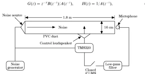
Voltage signals were used as the reference input so that acoustic feedback could be ignored. The algorithms were implemented on a 32-bit floating point digital signal processor TMS320C31 in conjunction with two-channel analog inputs and two-channel analog outputs. A circular PVC duct of length 1·8 m and diameter 16 cm was chosen for the test. The corresponding cut-off frequency of the duct is 1075 Hz. This renders the effective control bandwidth below approximately 1 kHz, where only plane waves are of interest. A third order Bessel filter was used as the anti-aliasing filter. The ANC system, including the digital controller, the signal conditioning circuit, the sensor and the actuator, is schematically shown in Figure 2. Four ANC algorithms were employed to suppress various synthetic noises and practical noises. The synthetic noises include a white noise and a sweep sine, while the practical noises include an engine noise, a blower noise and an impact noise. When implementing the digital controllers, the models of P(z) and S(z) must be determined prior to finding C(z). To this end, a parametric system identification procedure was employed to establish a mathematical model of the coupled transducer–duct system. This method can be more practical than analytical methods and numerical methods for complex systems. Suppose that the input signal to the system and the output signal from the system are discretized into u(k) and y(k), respectively, by some data acquisition system. Then a parametric model is estimated on the basis of these input and output data sampled in the time domain. The white noise is selected as the input signal since it satisfies the condition of persistent excitation, as required by a reliable identification [19]. The parametric model that is adopted in this study is the autoregressive with exogenous input (ARX) model [19]

y(k) = G(z)u(k) + H(z)e(k), k= 1, 2, . . . ,a, (15) where z is the shift operator, G(z) is the plant transfer function to be identified and H(z) is the transfer function associated with the disturbance process. In the ARX model, the transfer functions G(z) and H(z) take the forms

G(z) = z−N_B(z−1_)/A(z−1_{), H(z) = 1/A(z}−1_{), (16)}

where N is the delay in samples, A(z−1_{) and B(z}−1_{) are polynomials in z}−1_{, i.e.,} A(z− 1_{) = 1 + a}

1z− 1+ · · · + anaz− na, B(z−1) = b1+ b2z−1+ · · · + bnbz−nb + 1, (17)

with the numbers na and nb − 1 being the orders of respective polynomials. Hence, the model in equation (15) can be written as

A(z−1_{)y(k) = B(z}−1_{)u(k − nk) + e(k). (18)}

The identification procedure consists mainly of estimating these na + nb parameters involved in the ARX model by, for example, the least squares method. Details can be found in reference [19].

For the transducer–duct systems, the aforementioned parametric identification procedure was employed to set up the corresponding mathematical models. First, white noise was used to excite the duct under test. The input data and the output data were then recorded by a signal analyzer, based on a sampling rate of 4 kHz. Second, the orders and the delay of the ARX model were adjusted. This process might take several iterations until the magnitude and the phase of the measured and the regenerated frequency response functions were well matched, and the ARX model orders were then selected according to

T 1

The models of the primary path and the cancellation path identified by the ARX procedure

P(z) S(z)

ZXXXXXXXXCXXXXXXXXV ZXXXXXXXXCXXXXXXXXV

Zeros Poles Zeros Poles

−0·90852 0·2484j −0·01592 0·9580j −0·5942 −0·07942 0·9709j −0·85992 0·0276j −0·07612 0·9761j −1·3777† −0·22182 0·9533j −0·76542 0.4859j −0·21512 0.9542j −1·02622 0·0927j† −0·33002 0·9160j −0·66552 0.5896j −0·32342 0.9195j −0·95952 0·3029j† −0·45422 0·8738j −0·56162 0.7809j −0·45822 0.8561j −0·91892 0·4777j† −0·58722 0·7683j −0·34662 0.8467j −0·56602 0.7935j −0·74112 0·6213j −0·52422 0·7111j −0·14462 0.9124j −0·57862 0.7059j −0·66702 0·7666j† −0·66512 0·7078j −0·04362 0.5133j −0·66832 0.6739j −0·48872 0·8228j −0·75402 0·6031j 0·02182 0.9708j −0·76772 0.5889j −0·43282 0·8368j −0·82682 0·4971j 0·93892 0.3521j† −0·82142 0.4762j −0·25882 0·9610j −0·86452 0·4031j 0·79262 0.4313j −0·85072 0.3580j −0·08252 0·9849j −0·91522 0·2808j 0·59442 0.8037j −0·91552 0.2452j 0·11382 0·9892j −0·95672 0·1990j 0·63602 0.5754j −0·89262 0.2094j 0·29802 0·9519j −0·96942 0·0730j 0·41482 0.7333j −0·95412 0.0677j 0·35002 0·4867j 0·98322 0·0562j 0·24052 0.7982j 0·97692 0.0582j 0·46922 0·87161 0·95512 0·1932j 1.0791† 0·94742 0.1724j 0·63362 0·7657j 0·93582 0·3056j 0.9569 0·92012 0.3189j 0·76862 0·6324j 0·89802 0·4139j 0·88912 0.4128j 0·87352 0·4706j 0·86572 0·4780j 0·86802 0.8419j 0·94412 0·2964j 0·79242 0·5987j 0·79222 0.5987j 1.0263† 0·71622 0·6873j 0·71612 0.6866j 0.9943 0·62012 0·7759j 0·62162 0.7765j 0.4495 0·54002 0·8243j 0·53302 0.8231j 0·46852 0·8645j 0·47212 0.8679j 0·33602 0·9278j 0·33802 0.9301j 0·22062 0·9591j 0·22162 0.9600j 0·08932 0·9845j 0·08932 0.9883j 0·00742 0·9800j 0.8576 0.2759

Delay = 24, gain = 0·5247 Delay = 12, gain = 0·3242 †Denotes non-minimum phase zeros

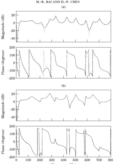
Figure 3. A comparison between the measured and the regenerated frequency response functions. (a) The frequency response function between the primary noise and the sensor: P(ejv_{); (b) the frequency response function}

between the cancelling loudspeaker and the sensor: S(ejv_{). (—), Measured data; (- - -), regenerated data.}

Akaike’s information-theoretic criterion (AIC) [19]. The poles and zeros of the transfer functions of the primary path and the cancellation path identified by using the ARX model as shown in Table 1, and their frequency response functions are shown in Figure 3. Note that there are 11 NMP zeros in the plant S(z). Excellent agreement was obtained between the measured and the regenerated frequency response functions except for the frequency range below approximately 50 Hz, in which the loudspeakers exhibited poor low frequency response. Consequently, the control bandwidth was restricted to approximately 50–800 Hz in the study

In order to compare different ANC algorithms, five types of noises were used as the primary disturbance. The first two, including a Gaussian white noise and a sweep sine, are synthetic noises. The remaining three, including an engine noise, a blower noise and an impact noise, are experimental data. In what follows, the results obtained from five ANC experiments will be presented.

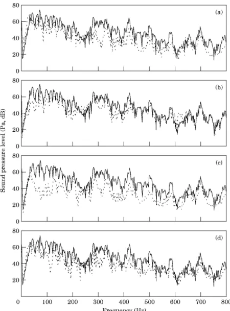
In the first case, a Gaussian white noise was used as the primary noise. The sound pressure spectra before and after ANC is activated are shown in Figure 4. Significant

attenuation (from 50–800 Hz) was obtained by using four ANC methods. Among the methods, the H2 method appears to provide best attenuation at low frequencies

(approximately 30–240 Hz). Questions will naturally arise: Did the H2 design actually

minimize the 2-norm of the model matching error, and Ha thea-norm? The answer is yesin theory and no in reality. Theoretically, the Ha controller minimizes the maximum

error in the model matching so that the resultant error function becomes an all-pass function [12], which somewhat contradicts the experimental results in Figure 4(d). This discrepancy can be accounted for in several ways. There is error between the mathematical model and the actual plant. Numerical errors seem to be unavoidable, since the acoustic plants are of extremely high order in respect to the complexity of the controller synthesis. This is not to mention a pitfall in the present methods, which is to be fixed in future study: that is, the calculated controllers tend to produce excessive gains at high frequencies so

Figure 4. The sound pressure spectra for the Gaussian white noise before (—), and after (- - -) ANC is activated. (a) Roure’s method; (b) FXLMS method; (c) H2method; (d) Hamethod. The step size in FXLMS

as to compensate for the NMP zeros. An heuristic approach employed in this study is to truncate judicially the high frequency components of the controllers which are inversely Fourier transformed to obtain the impulse response that in turn is used for the coefficients of FIR filters. This is especially relevant for broadband random noise attenuation, such as the white noise in this case. All of these factors will inevitably contribute to the difference between the experimental results and the theoretical predictions in the application of the

Ha method, and also in the other methods.

In the second case, a sweep sine described by the following equation was used as the primary noise:

0·027 sin [2p(100t2_{+ 200t)]. (19)}

Figure 5. The time domain response for the sweep sine before (—) and after (- - -) ANC is activated. (a) Roure’s method; (b) FXLMS method; (c) H2method; (d) Hamethod. The step size in FXLMS is 0·005 and the filter

The sinusoidal noise sweeps from 200 Hz in a rate 100 Hz/s to 300 Hz. This type of noise generally occurs during machine run-up or automobile acceleration. The time domain response of the sweep sine case before and after ANC is activated is shown in Figure 5. All methods except the FXLMS method produce satisfactory attenuation.

In the third case, an exhaust noise from the gasoline engine of a 2000 c.c. automobile operating at 4000 rpm was chosen as a more practical primary noise. The sound pressure spectra before and after ANC is activated are shown in Figure 6. All methods provide significant attenuation. In particular, the H2 method appears to give slightly more

attenuation at low frequencies (approximately 40–240 Hz) than the other methods. The FXLMS give significant attenuation at peaks, as expected.

Figure 6. The sound pressure spectra for the engine noise before (—) and after (- - -) ANC is activated. (a) Roure’s method; (b) FXLMS method; (c) H2method; (d) Hamethod. The step size in FXLMS is 0·005, the

In the fourth case, the noise from a blower with a radial fan operating at 3000 rpm is used as the primary noise. The noise contains harmonics associated with the blade-passing frequency and broadband components due to turbulence. The second pressure spectra before and after ANC is activated are shown in Figure 7. All methods provide significant attenuation. In particular, the H2 method appears to give more attenuation at low

frequencies (approximately 50–200 Hz) than the other methods.

In the final case, an impact noise from a forge hammer in a shipyard was chosen as the primary noise. The reason for choosing the impact noise is because it represents a large class of transient noises. For example, the impact noise of punch presses, the noise of forge machines, the noise of gun shot, and the tunnel noise of high speed trains all fall into this category. This particular type of application has rarely been investigated in ANC research

Figure 7. The sound pressure spectra for the blower noise before (—) and after (- - -) ANC is activated (a) Roure’s method; (b) FXLMS method; (c) H2method; (d) Hamethod. The step size in FXLMS is 0·1, the

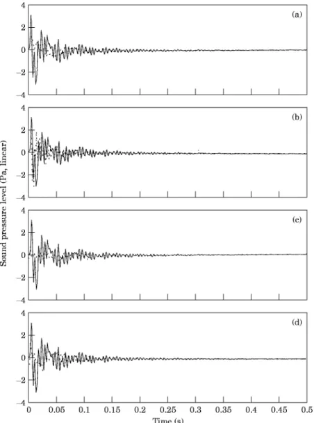
to date, because it involves difficulties of control methods and transduction. In the study, we attempted to use the developed algorithms to attack the practical noise problem. The time domain response of the impact noise before and after ANC is activated is shown in Figure 8. All methods except the FXLMS method produce satisfactory attenuation. It should be noted that, although the FXLMS method is too sluggish to respond to this impact noise, it should work for cases involving repetitive pulses with sufficiently short period if enough time is provided for adaptation.

3.2.   

From the experimental results, a comparison of four feedforward ANC approaches is in order. In general, the design complexity of the H2and Hacontrollers is higher than those

Figure 8. The time domain response for the impact noise before (—) and after (- - -) ANC is activated. (a) Roure’s method; (b) FXLMS method; (c) H2method; (d) Hamethod. The step size in FXLMS is 0·05 and

of the other methods. However, the computation load and I/O channel number (see Figure 2) of the proposed methods are lower than that of the FXLMS method. This is due to the fact that the former require only a digital filter, while the FXLMS method requires two digital filters (for filtered-x operation and filter output convolution, respectively) and a filter weight update procedure. Nevertheless, the FXLMS has certain advantages over the other methods, while makes it still a widely used technique in the ANC community. The most significant feature of the FXLMS is considered to be its adaptive property that is important in practical applications. However, it should be noted that the FXLMS adapts only to the filtered disturbance, but not to the plant (the cancellation path) itself, provided that the plant is identified off-line. If deviation of the plant arises, e.g., change of effective delay, the performance of the FXLMS algorithm may be degraded, especially for broadband random noises. The reason for this is that perturbations to the plant will alter the instantaneous search direction in FXLMS. In addition, it generally takes several iterations to determine an appropriate step size in the FXLMS method for each particular type of noise, such that a reasonable compromise between the convergence speed and the stability can be achieved.

On the other hand, Roure’s methods, and the H2and Hamethods, are essentially fixed

controllers which do not depend on any particular type of input noise. In addition, both analog controllers and digital controllers can be implemented by using these fixed controllers. This feature may be desirable in practical applications because, for example, it could be more economical to use an analog ANC device in an electronic ear-muff than the digital counterpart.

From the experimental results, all methods provide significant attenuation for white noise, engine noise and blower noise. In particular, the H2method and the FXLMS method

appeared to give better attenuation at low frequencies than the others. However, one should not draw a general conclusion based on the experimental result, which is case-dependent.

Roure’s method, and the H2 and Ha methods exhibit effectiveness in suppressing

transient noise, e.g., the aforementioned sweep sine and the impact noise, since they are all fixed controllers. In addition, unlike FXLMS, these methods do not suffer from the problem of non-uniform convergence due to eigenvalue disparity [15]. A detailed comparison of the H2and Hamethods would show that the former provides better low

frequency performance than the latter. This is because the Ha method (designed for the

worst case input) is being somewhat conservative, and it generally exerts more control effort on NMP zeros that exist at high frequencies [12].

T 2

Summary of the characteristics of the ANC techniques

Algorithm characteristics Roure FXLMS H Ha

Design complexity Low Low Medium High

Computation load Low HIgh Low Low

I/O 1 in/1 out 2 in/2 out 1 in/1 out 1 in/1 out

Adaptive No Partially No No

Input-dependency No Yes No No

Analog(s)/digital (z) control s/z z only s/z s/z

Deals with transients Yes No Yes Yes

Eigenvalue disparity No Yes No No

One last remark is concerned with robust stability. By definition, a controller provides robust stability if it provides stability for a set of plant [12]. Roure’s method and the H2

and Ha methods, do not have the problem of robust stability, since they are purely

feedforward, and both the primary path and the cancellation path consist only of stable components. The overall system is always stable regardless of the change of the plant, except that the performance might degrade. On the other hand, the FXLMS does have the problem of robust stability because the algorithm can be shown to be equivalent to a feedback system [20]. It is possible that the adaptation diverges and the overall system becomes unstable if the plant drifts too much from the nominal one.

The above-mentioned characteristics of the ANC techniques are summarized in Table 2. It should be pointed out that the features included in Table 2 are only objective comparisons. In practical applications, none of the methods holds absolute superiority over the others, and the choice is really a matter of taste.

4. CONCLUSIONS

In this study, two novel techniques on the basis of the feedforward H2and Haoptimal

model matching principles have been developed. ANC systems for duct noises based on the H2 and Ha algorithms are realized by using a digital signal processor. The

characteristics of the proposed methods have been compared with those of Roure’s method and the FXLMS method. The experimental results indicate that the proposed methods provide noise attenuation comparable to those of the other two methods. In addition, the proposed methods exhibit great potential in actively supressing transient noises that frequently arise in practical applications. However, as a limitation of the proposed methods, the performance may degrade if the plant excessively drifts from the nominal one. This drawback of the current methods can possibly be eliminated by on-line identification to avoid instability due to the plant drifting from the nominal one. Development of adaptive techniques based on the Hand Ha algorithms is also under way.

ACKNOWLEDGMENTS

Special thanks are due to Professors F. B. Yeh and J. S. Hu for the helpful discussions on the H2 and Ha control theories. The work was supported by the National Science

Council in Taiwan, Republic of China, under the project number NSC 83-0401-E-009-024.

REFERENCES

1. P. L 1936 U.S. Patent No. 2043416. Process of silencing sound oscillations.

2. P. A. N and A. J. E 1992 Active Control of Sound. London: Academic Press. 3. S. J. E and P. A. N 1994 Noise/News International 2, 75–98. Active noise control. 4. M. O. T and R. R. L 1992 Active Noise Control. Oxford: Clarendon Press. 5. A. R 1985 Journal of Sound and Vibration 101, 429–441. Self-adaptive broadband active

sound control system.

6. D. R. M 1980 IEEE Transactions on Acoustics, Speech, and Signal Processing ASSP-28, 454–467. An analysis of multiple correlation cancellation loops with a filter in the auxiliary path. 7. B. W and S. D. S 1985 Adaptive Signal Processing. Englewood Cliffs, NJ:

Prentice-Hall.

8. J. C. B 1981 Journal of the Acoustical Society of America 70, 715–726. Active adaptive sound control in a duct: a computer simulation.

9. L. J. E, M. C. A and R. A. G 1987 IEEE Transactions on Acoustics, Speech, and Signal Processing 35, 433–437. The selection and application of an IIR adaptive filter for use in active sound attenuation.

10. M. M and E. Z 1989 Robust Process Control. Englewood Cliffs, NJ: Prentice-Hall. 11. G. F. F, J. D. P and A. E-N 1994 Feedback Control of Dynamic

Systems. Reading, MA: Addison-Wesley.

12. J. C. D and B. A. F 1992 Feedback Control Theory. New York: Maxwell-Macmillan International.

13. J. S. F 1985 IEEE Transactions on Automatic Control AC-30, 555–565. Right half plane poles and zero design tradeoffs in feedback systems.

14. D. K. M 1991 Journal of Dynamic Systems, Measurement, and Control 113, 419–424. Physical interpretation of transfer function zeros for simple control systems with mechanical flexibilities. 15. P. M. C 1993 Optimal and Adaptive Signal Processing. London: CRC Press. 16. B. A. F 1987 A Course in HaControl. Lecture Notes in Control and Information Science

88. New York: Springer-Verlag.

17. F .B. Y and C. D. Y 1991 Post Modern Control Theory and Design. Taiwan: Eurasia. 18. J. B. G 1981 Bounded Analytic Functions. New York: Academic Press.

19. L. L 1987 System Identification: Theory for the User. Englewood Cliffs, NJ: Prentice-Hall. 20. E. F. B, R. B. C and A. A. O 1995 The 1995 International Symposium on Active Control of Sound and Vibration, Newport Beach, U.S.A., 1149–1159. Trade-off between using the feedforward Widrow filtered-x LMS algorithm and a compensator/regulator feedback algorithm for narrowband control.