適用於網路多媒體之可調式誤碼校正機制設計

國

立

交

通

大

學

電 機 與 控 制 工 程 學 系

碩

士

論

文

適用於網路多媒體之

可調式誤碼校正機制設計

Adaptive Forward Error Correction for

Internet Multimedia

研 究 生：曾勁源

指導教授：黃育綸 博士

適用於網路多媒體之

可調式誤碼校正機制設計

Adaptive Forward Error Correction for

Internet Multimedia

研 究 生：曾勁源 Student：Chin-Yuan Tseng

指導教授：黃育綸 博士 Advisor：Dr. Yu-Lun Huang

國 立 交 通 大 學

電機與控制工程學系

碩 士 論 文

A Thesis

Submitted to Department of Electrical and Control Engineering College of Electrical Engineering and Computer Science

National Chiao Tung University in Partial Fulfillment of the Requirements

for the Degree of Master

in

Electrical and Control Engineering

July 2007

Hsinchu, Taiwan, Republic of China

適用於網路多媒體之

可調式誤碼校正機制設計

學生：曾勁源 指導教授：黃育綸 博士

國立交通大學 電機學院 電機與控制工程研究所

摘 要

可調式誤碼校正(Adaptive Forward Error Correction, 簡稱 AFEC)是一種利用動 態評估網路狀態調整冗餘封包數量，以達到提升接收端播放品質的機制。一般而言， AFEC 常用在有即時性需求的網路服務中，特別是在多媒體服務方面的應用。因為網路 服務的即時性的要求，所以當封包遺失時，將無法透過一般的重傳機制重新取得遺失的 封包。因此，在AFEC 中，不採用重傳機制和服務品質(Quality of Service, 簡稱 QoS)的 方式確保服務品質，而是改用動態評估及預測網路擁塞狀況，並以複製封包的方法調整 冗餘封包的數量，讓接收端能即時取得遺失的封包以提升接收品質。然而，AFEC 在網 路環境評估與預測的準確性上常有誤差，使得接收端並無法有效率地利用冗餘封包來回 復遺失的資料。換句話說，一旦因評估錯誤而造成注入過多的冗餘封包，不僅無法有效 率的提升接收品質，反而會造成更嚴重網路擁塞情形。因此本論文提出了一套數學模 型，目的在找出冗餘封包數量和接收品質的最佳平衡點。為此，我們設計了可套用到 AFEC 中的可調式回饋控制方法，提出了三種機制，能動態地依據網路現狀調整冗餘封 包數量，以達到提升接收品質，避免造成網路擁塞的目的。除此之外，由於注入冗餘封 包的緣故，單位時間內所能傳送的有效資料量也隨之減少，因此，本論文中也特別分析 了冗餘封包與接收品質之間的關係，期望提供服務商注入冗餘封包，提升接收品質時的 參考依據。

Adaptive Forward Error Correction for

Internet Multimedia

Student: Chin-Yuan Tseng Advisor: Yu-Lun Huang

Department of Electrical and Control Engineering

National Chiao Tung University

Abstract

By injecting redundant packets, adaptive forward error correction (AFEC) mechanisms recover the lost packets at the receiver side and thus improve the receiving qualities of real-time applications over unreliable packet networks. In this paper, we propose a simple mathematical equation of packet loss rate, receiving quality and transmission overhead to find the optimal redundancy solution for real-time applications. In addition, three adaptive control schemes are presented based on the proposed equation: static, dynamic and advanced AFEC schemes. In these proposed schemes, the data block size, redundancy overhead and qualities can be adjusted based on the estimated loss rate and network status. Upon applying these schemes, the receiving qualities of real-time applications can be guaranteed by recovering the lost packets with the redundant ones. Compared with non-AFEC mechanisms, the simulation results also show that the proposed schemes effectively improve the receiving qualities with good performance and packet redundancy.

Acknowledgement

First, I would like to show my sincere gratitude to my thesis advisor, Dr. Yu-Lun Huang who supported my research and guided me patiently. My thanks also go to the seniors who I worked with at the lab for the projects funded by Institute for Information Industry. This valuable chance in my first year enabled me to learn how to analyze and solve problems in programming which later strengthened my research and writing ability in my own research. I could not have completed my thesis without the valuable suggestions of my advisor, the seniors at the RTES lab and my friends. I have benefited a lot from their warm support through the process of my thesis writing.

These two years at NCTU is the highlight of my life. I owe a debt of gratitude to Dr. Yu-Lun Huang. Thanks are extended to the seniors- 瀞瑩, 志堅 and 嘉良; my friends- 建銘, 精佑, 欣宜, 依文, 恩捷, 詠文, 培華, 興龍, 立穎, Newlin, Shylu, and Joyce. I also want to express my deep appreciation to my family who encouraged me to achieve my goal and comforted me when I was stressed.

Lastly I would like to thank everyone again for inspiring and motivating me to do the best work which helped me to complete this thesis within two years.

Table of Contents

Abstract (Chinese) ...i

Abstract (English)...ii

Acknowledgement ...iii

Table of Contents...iv

List of Tables ...vi

List of Figures...vii

Chapter 1 Introduction ...1

Chapter 2 Related Work ...2

2.1 Internet Multimedia ...2

2.2 NS-2...3

2.3 RTP/RTCP ...4

2.4 FEC...9

2.5 AFEC...10

2.5.1 A New Feedback Control Mechanism... 11

2.5.2 Enhanced Adaptive FEC (EAFEC) ...13

2.6 Summary...15

Chapter 3 H-Q Equation...16

3.1 Static AFEC (SAFEC) ...19

3.2 Dynamic AFEC (DAFEC)...21

3.3 Advanced AFEC (AAFEC) ...22

3.4 Summary...23 Chapter 4 Simulation...24 4.1 Configuration...24 4.2 Simulation...25 4.2.1 NS-2 Files...26 4.2.2 RTP Sessions ...27 4.2.3 Tcl Scripts ...28 4.3 Simulation Results...32 4.3.1 Output Files ...32 4.3.2 Network Animator ...34 4.4 Summary...35

Chapter 5 Analysis and Comparison...36 5.1 Analysis ...36 5.1.1 SAFEC...36 5.1.2 DAFEC ...39 5.1.3 AAFEC ...40 5.2 Performance Analysis...42 5.3 Comparison...44 5.4 Summary...48 Chapter 6 Conclusions ...49

Chapter 7 Future Work ...50

References ...51

List of Tables

Table 3.1 Notation Definition...16

Table 4.1 Nam partial symbol table...33

Table 4.2 H-Q equation for AFEC schemes analysis data list...33

Table 5.1 Comparison of FEC and AFEC schemes...45

Table 5.2 Comparison of adaptive controller and simulation result...46

Table 5.3 Performance of FEC and AFEC on loss rate 50%...47

List of Figures

Figure 1.1 Redundant RTP packets ...2

Figure 2.1 NS-2 architecture ...3

Figure 2.2 Trace format example...4

Figure 2.3 Network animator ...4

Figure 2.4 RTP header format ...5

Figure 2.5 Network protocol architecture ...6

Figure 2.6 RTP packet ...6

Figure 2.7 RTCP payload format...7

Figure 2.8 RTCP sender report format ...8

Figure 2.9 RTCP receiver report format ...9

Figure 2.10 FEC Packet structure...10

Figure 2.11 FEC parity header format...10

Figure 2.12 AFEC flowchart ... 11

Figure 2.13 Error correction ...12

Figure 2.14 Object function J as a function of fixed redundancy u and independent packet loss with fixed probability p ...13

Figure 2.15 Wireless AP adds redundant FEC data to video transmission data ...14

Figure 2.16 FEC redundant packet numbers in the EAFEC algorithm...14

Figure 2.17 Simulation topology...14

Figure 3.1 Transmitted packets...17

Figure 3.2 Relationship among H, L and Q...18

Figure 3.3 Adaptive control of AFEC in sender side...19

Figure 3.4 Adaptive control of SAFEC flowchart...20

Figure 3.5 Adaptive control of DAFEC flowchart ...21

Figure 3.6 Adaptive control of advanced AFEC flowchart ...22

Figure 4.1 Simulation environment ...25

Figure 4.2 RTP session with AFEC of NS-2 ...27

Figure 4.3 AFEC simulation...34

Figure 5.1 SAFEC vs. non-AFEC ...36

Figure 5.3 SAFEC performance analysis ...38

Figure 5.4 SAFEC packet redundancy analysis ...38

Figure 5.5 DAFEC performance ...39

Figure 5.6 DAFEC packet redundancy ...40

Figure 5.7 AAFEC performance...41

Figure 5.8 AAFEC packet redundancy...41

Figure 5.9 Three AFEC various performance ...42

Figure 5.10 Three AFEC schemes packet redundancy analysis...43

Figure 5.11 Network environment...44

Chapter 1

Introduction

Internet multimedia is one of the most popular applications in the 21st century; subscribers are able to access internet multimedia contents, such as voice-over-IP (VoIP), video-on-demand (VoD), through their mobile devices. With the growth of subscribers of internet multimedia, the requirement of network bandwidth is increasing and thus the real-time delivery of multimedia contents becomes one of the major challenges for their service providers. To improve the quality of perception, the real-time transport protocol (RTP) [1-4], which has less overhead in packet transmission, is widely adopted for the end-to-end content delivery. However, RTP neither guarantee timely delivery nor quality of service (QoS).

To guarantee real-time delivery and the perception quality, researchers propose many methods and schemes in the past few years. In 1997, K. Park and W. Wang proposed packet-level forward error correction (FEC) [5], [6] scheme by using redundant packets to recover the lost packets based on the original estimation of network quality, and thus enhance the perception quality in the destination devices. However, the number of the redundant packets estimation in FEC does not change according to the network environment and thus may inject a lot of overhead in data communication. In the same paper, the adaptive forward error correction (AFEC) [7] protocol is also proposed to adaptively change the estimated number of the redundant packets in FEC scheme. It is widely used to facilitate the end-to-end transport of real-time traffic by leveraging the redundancy of packets. In the same year, C. Perkins et al. proposed a RTP payload format for encoding redundant audio data to enhance the audio quality, as shown in Figure 1.1.

Figure 1.1 Redundant RTP packets

However, there exists a tradeoff between the overhead caused by injecting the redundant packets and the perception quality. Recently, many researches focus on the discussion of methods to gain the optimal perception quality with less overhead caused by the redundant packets. In this paper, we propose a mathematical method which can dynamically change the number of redundant packets and gain the optimal perception quality. The proposed adaptive control schemes are simulated by using Network Simulation version 2 (NS-2) [8-10] and are proofed to be efficient enough about adaptive controller for end-to-end network transmission.

Chapter 2

Related Work

To improve the perception quality, reduplicating packets is implemented in many systems. However, these redundant packets also result in transmission costs and overheads to the network. To keep balance of quality and overhead, the AFEC protocol proposed by K. Park and W. Wang depicts a concept to adaptively change the estimated number of the redundant packets. An adaptive control module is added to the FEC protocol and used to receive the status reports from the receiver. Thus, the packet redundancies in AFEC can be adaptively determined according to the current network status. However, it only presents a comprehensive controlled simulation study of AFEC.

2.1 Internet Multimedia

The receiving quality is one of the major concerns in delivering multimedia contents over the internet. The enhancement of the receiving quality is the main point of this paper. Internet multimedia [11] has time constraint issue [12-16], so-called real-time delivery of traffic requires little in the way of transport protocol. In particular, real-time constraint traffic that is sent to far away distances without re-transmittable. Therefore, there are some facets of an end-to-end protocol need to be re-designed or refined including separate flows for each media stream, receiver adaptation, and synchronization. The receiver adaptation is about real-time applications such as audio and video need to be able to buffer real-time data at the receiver for sufficient time to do some procedures to have better display at the receiver. The internet transport protocol for real-time flows is RTP. RTP provides end-to-end delivery services for real-time data, such as interactive audio and video streams. These services include payload type identification, sequence numbering, timestamping and delivery monitoring. Applications typically run RTP on top of UDP [17] to leverage their multiplexing and checksum services. Note that RTP itself does not provide any mechanism to ensure timely delivery or provide other quality-of-service guarantee, but relies on lower-layer services to do so. Each RTP flow is supplemented by RTCP [18] packets. The data transport is augmented by a control protocol, like RTCP, to allow monitoring of the data delivery in a manner scalable to large multicast networks, and to provide minimal control and identification functionality.

2.2 NS-2

Network Simulator-version 2 (NS-2) is a discrete-event driven and object-oriented network simulator, written in C++, with an OTcl (Object-Oriented Tool Command Language) interpreter as a front end (Figure 2.1). The simulator supports a class hierarchy in C++, and similar class hierarchy within the OTcl interpreter. NS-2 uses two languages because simulator has two different kinds of things it needs to do. One is detailed simulations of protocols requires a systems programming language which can efficiently manipulate bytes, packet headers, and implement algorithms that run over large data sets. The other one is a large part of network research involves slightly varying parameters or configuration, or quickly exploring a number of scenarios.

Figure 2.1 NS-2 architecture

NS-2 can trace the events of network simulation. Figure 2.2 shows that the event tracing data format.

Figure 2.2 Trace format example

Network animator (Nam) of NS-2 (Figure 2.3) can provide a Graph User Interface (GUI). Nam is a Tcl/TK based animation tool for viewing network simulation traces and real world packet traces. It supports topology layout, packet level animation, and various data inspection tools [19].

Figure 2.3 Network animator

2.3 RTP/RTCP

RTP provides end-to-end delivery services for real-time data, such as interactive audio Session/RTP

Session/RTP Session/RTP

and video streams. RTP header format as Figure 2.4 includes payload type identification, sequence numbering, timestamping and delivery monitoring.

¾ Timestamp

– Purpose : reduce/erase jitter – Initial value is random

– Sampling instant MUST be derived from a sampling clock (Sampling clock ≠ system clock)

– Increment monotonically

– Linearly in time to allow synchronization – Jitter calculations

¾ Sequence number

– Purpose : restore packet sequence – Initial value is random (unpredictable) – Detect packet loss

Figure 2.4 RTP header format

Applications typically run RTP on top of UDP (Figure 2.5, Figure 2.6) to leverage their multiplexing and checksum services. Note that RTP itself does not provide any mechanism to ensure timely delivery or provide other quality-of-service guarantee, but relies on lower-layer

services to do so.

Figure 2.5 Network protocol architecture

Figure 2.6 RTP packet RTP provides means for:

– Jitter elimination/reduction

– Synchronized playback of a source’s audio and video can be achieved using timing information carried in the RTCP packets (Figure 2.7) for both sessions.

– Multiplexing is provided by the destination transport address (network address and port number) which is different for each RTP session.

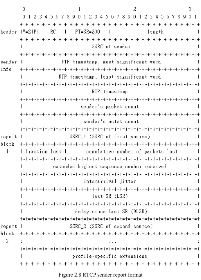
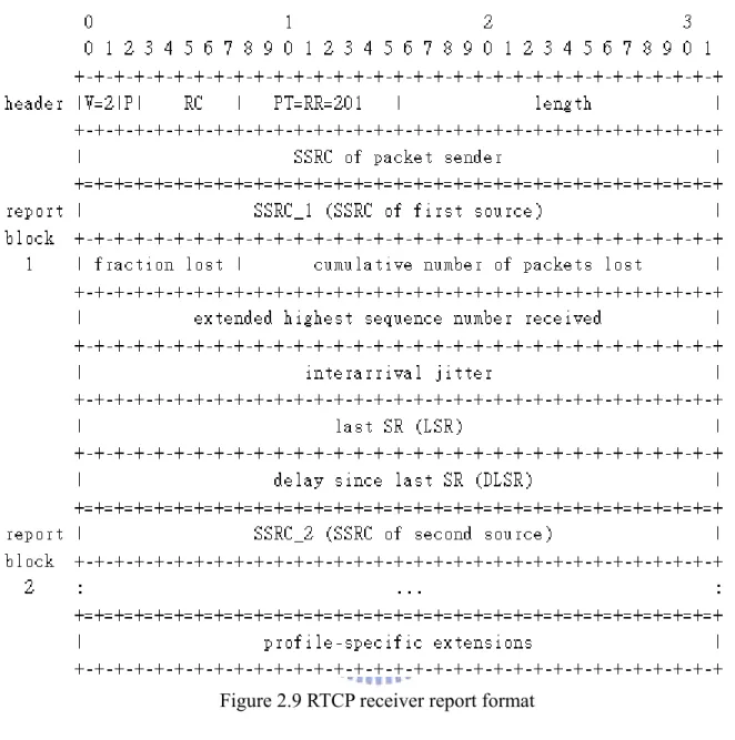
The data transport is augmented by a control protocol (RTCP) sender report (Figure 2.8) and receiver report (Figure 2.9) to allow monitoring of the data delivery in a manner scalable to large multicast networks, and to provide minimal control and identification functionality.

RTCP performs four functions

– Primary function : provide feedback on the quality of the data distribution (related to the flow and congestion control function)

– Carries a persistent transport-level identifier for an RTP source called the canonical name or CNAME

– Flow control : The first two functions require that all participants send RTCP packets, therefore the rate must be controlled in order for RTP to scale up to a large number of participants. This number is used to calculate the rate at which the packets are sent.

– OPTIONAL function is convey minimal session control information

Figure 2.7 RTCP payload format

8 bytes Min. 12 bytes Variable, 32-bits boundary UDP header RTCP header RTCP payload

Figure 2.9 RTCP receiver report format

2.4 FEC

RFC 3452 specifies a payload format for generic forward error correction (FEC) (Figure 2.10) of media encapsulated in RTP. It is engineered for FEC algorithms based on the exclusive-or (parity) operation. It also allows for the recovery of both the payload and critical RTP header (Figure 2.11). It generic means that the FEC protocol is (1) independent of the nature of media being protected, be it audio, video, or otherwise, (2) flexible enough to support a wide variety of FEC mechanisms, (3) designed for adaptively so that the FEC technique can be modified easily without out of band signaling, and (4) supportive of a number of different mechanisms for transporting the FEC packets.

Figure 2.10 FEC Packet structure

SN base(16bits) Length recovery(16bits)

E PT recovery(7bits) Mask(24bits)

TS recovery(32bits)

↑

12 bytes

↓

Figure 2.11 FEC parity header format

2.5 AFEC

AFEC (Adaptive Forward Error Correction) protocol is for packet-level forward error correction in dynamic networks. It is used to facilitate end-to-end transport of real-time traffic whose timing constraints rule out the use of retransmission-based congestion control and quality of service (QoS) provision schemes. The difference between AFEC and FEC is that the redundant packet size in AFEC can be dynamically changed base on the network factors, delay, loss and jitter. It has well-behaved in dealing with network congestion and packet recovery rate than FEC. To make the network connection more reliable and robust by leveraging the redundancy of data packets becomes an important issue in real-time applications.

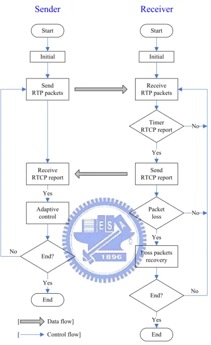
Figure 2.12 is general AFEC design flowchart. Sender needs to initialize parameters like quality, packet loss rate, original data packets length, and the number of redundant packets. The method of sending RTP packets is redundant packets coming after original packets. Redundant packets use randomly choice from original packets. At the same time, the sending job would be interrupted when receiving RTCP (Real-Time Control Protocol) report packets. The information of RTCP report packets include receiving quality which calculated in receiver. The sender can calculate the number of redundant packets based on receiving quality. The transmission stops until receiving communication ending message. The receiver needs to initialize parameters, too. These parameters include receiving quality, receiving queue, and recovery queue. Receiver needs to receive RTP packets and check packets loss event all the time. The receiving job would be interrupted when RTCP report timer rising. At this time, the receiver needs to calculate the receiving quality relies on number of receiving packets and lost packets, and then embedding this receiving quality information in the RTCP report. The

transmission stops until receiving communication ending message. Start Initial Send RTP packets Adaptive control End? End Yes Yes Start Initial Receive RTP packets Timer RTCP report Send RTCP report End? End Yes Yes Packet loss Loss packets recovery Yes No No No No Receive RTCP report [ Data flow] [ Control flow] Sender Receiver

Figure 2.12 AFEC flowchart

2.5.1 A New Feedback Control Mechanism

In 2005, Oscar Flardh et al. propose a feedback controller [20-23] for the adaptive control module in AFEC. The authors proposed a model of packet loss to find the optimal redundancy as a function of packet loss probability. The proposed controller can be used to track the optimum using gradient estimation. To simplify the complication in the proposed controller and make the simulation workable, the authors make some unrealistic assumptions. For example, if the number of received packets is greater or equal than the original packets, then it

is assumed that no packet is lost during the transmission (Figure 2.13). However, the data recovery should depend on the losses of the data itself and its redundant packets. Data cannot be recovered if the data itself and its redundant packets are lost.

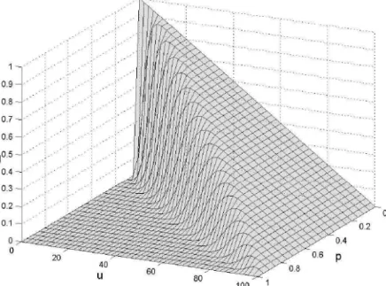
Figure 2.14 Object function J as a function of fixed redundancy u and independent packet loss with fixed probability p

In addition, the feedback controller tracks the optimum based on the feedback from receivers. However, the losses of these feedbacks, which may result in incorrect estimation, are not discussed in the paper. Moreover, the feedback controller has terrible performance when the network environment is suddenly changed, for example, when network congestion or router failures occurred.

2.5.2 Enhanced Adaptive FEC (EAFEC)

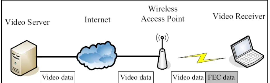
In 2006, Cheng-Han Lin et al. propose an Enhanced Adaptive FEC (EAFEC) algorithm [24] to improve video delivery quality over wireless networks. Video data transmitted over network as shown in Figure 2.15. It assumed that there is no packet loss in the video delivered path wired segment. The EAFEC algorithm in Figure 2.16 is hired in wireless AP side to video receiver. The algorithm can tune FEC packet redundancies in wireless Access Point (AP) by network traffic loads and wireless channel states to improve video delivery. The simulation topology shows as Figure 2.17. The simulation results show that the EAFEC improves system performances by dynamically tuning the FEC strengths. In the paper, four threshold values are used for the dynamic adjustments of packet redundancies in the proposed algorithm, EAFEC. These threshold values make the proposed algorithm easy to implement. However, the threshold values used in the algorithm come from the experimental results. It lacks of mathematical analysis and proof and cannot adapt to highly changeable network

environments.

Figure 2.15 Wireless AP adds redundant FEC data to video transmission data

Figure 2.16 FEC redundant packet numbers in the EAFEC algorithm

2.6 Summary

In this paper, we propose an equation based on the Poisson error model to evaluate the perception quality and adjust redundancy to transmitted data at the sender. Based on the equation, three AFEC schemes are also designed for the adaptive control module in AFEC. The three schemes are simulated on Real-Time Transport Protocol (RTP) data streams using NS-2 to improve the perception quality and reduce the packet redundancy. In the following sections, we depict the proposed equation, followed by the three schemes to adjust packet redundancy in AFEC.

Chapter 3

H-Q Equation

As mentioned in the above sections, trade-off exists in the perception quality and transmission overhead. In this paper, we propose a mathematical equation based on the changes between the transmission overhead (H) and quality (Q) to adaptively track the optimum of redundancies and provide better quality with lower overhead. The proposed equation is then named as H-Q equation. Before detailing the proposed equation, the notations used in this paper are briefed in Table 3.1.

Table 3.1 Notation Definition

Notation Description

B Original data block, the number of packets to be transmitted in a data block BL Lost packets, the number of lost packets in original data block

R Redundant packets, the number of redundant packets

N Transmitted packets, the total number of packets, including original and redundant

packets

ri Packet redundancy, the number of redundant packets for packet Pi

E(r) Expected packet redundancy, the expected value of packet redundancy

L Loss rate, the rate for packet loss during network transmission Q Receiving quality, the perception quality in receiver's side

QW Worse receiving quality, the worse quality that can be tolerated by receiving

applications

D Network delay time, the delay time (ms) in real network

Dmax Maximum network delay time that can be tolerated by applications

T Maximum processing time (ms) in receiver’s side, including queuing, searching,

etc

H Transmission overhead, the overhead resulting from injecting the redundant

packets

In the proposed equation, we assume that the redundant packets are randomly chosen from the packets, P1, P2… PB, in original data block and the packet redundancy, ri, is depending on

the previous receiving quality, Q, as shown in Figure 3.1. In this figure, R redundant packets are appended to the original data block, P1, P2… PB, and thus the total number of packets to

be transmitted become N, the summation of B and R.

Figure 3.1 Transmitted packets

Since the packet redundancy, ri, is assumed to be depending on the previous receiving

quality, Q, the expected value of packet redundancy, E(r), can be used to compute receiving quality and estimate the loss rate.

Assume that the redundant packets are randomly chosen from P1, P2… PB, the expected

value of the packet redundancy, E(r), can be derived according to the following equation Eq (1). B R r B r E B i i = =

∑

=1 1 ) ( Eq (1) Since E(r) represents the ratio of redundant packets and original packets, it can be considered as the transmission overhead, H, which is introduced by injecting redundant packets, as shown in Eq (2). B R r E H = ( )= Eq (2) In other words, an overhead H means there are H redundancies for each packet. In such a case, for each packet, there are totally H+1 copies transmitted over the network. Only if the

H+1 packets are totally lost, the receiving quality, Q, is affected. Therefore, it comes out the

following equation, Eq (3), named as H-Q equation. ) 1 ( ₋ +1 = H L Q Eq (3)

Furthermore, the overhead (H) and loss rate (L) can be derived from the above equation, as shown in Eq (4) and (5), respectively.

1 ) log( ) 1 log( − − = L Q H Eq (4) ) 1 ) 1 log( (

10

+ −

=

H Q

L

Eq (5) From the above equations, it is clear that the higher the loss rate is, the worse the receiving quality. To improve the receiving quality, it is possible to raise the redundancies, which result in higher overhead in the system. However, when injecting too many redundant packets, it makes network congestion and packet redundancy even worse. It helps nothing in improving the receiving quality. Figure 3.2 shows the relationship among receiving quality (Q), redundant overhead (H) and network loss rate (L). When transmission overhead is zero, receiving quality is monotonic decrease as packet loss rate gets higher. This H-Q equation can improve this situation. By injecting more transmission overhead, receiving quality curve can be enhanced. But receiving quality enhancement has limit, the curve through point A and B is an exponential curve which end off ∞ when packet loss rate gets higher.

Figure 3.2 Relationship among H, L and Q

improvement of receiving quality is limited even we inject more redundant packets and raise the transmission overhead. Thus, it is important to dynamically adjust the redundancies according to the loss rate and get the optimum in overhead and receiving quality.

In AFEC, it is important to get the balance between the perception quality and overhead, according to the packet loss rates. In this paper, the H-Q equation is proposed based on the above factors to implement the adaptive control in AFEC (Figure 3.3), described in the following sections. Start Initial Send RTP packets Adaptive control Receive BYE End Yes Yes No Receive RTCP report

Figure 3.3 Adaptive control of AFEC in sender side

3.1 Static AFEC (SAFEC)

The proposed static AFEC (SAFEC) can be applied to applications with static sized data blocks. It repeatedly estimates the receiving quality and packet loss rate to determine the packet redundancies to get an optimal between overhead and receiving quality. In SAFEC, shown in

Figure 3.4, it checks current receiving quality to see if it reaches the worse receiving quality (QW) or not. If QW≦Q, it means that network status is better than expected, and the

packet redundancies can be reduced according to the equation, Eq(4), where Q equals to QW.

This lowers down the network congestion and packet redundancy. On the contrary, when the packet loss rate is worse than expected, the packet loss rate should be re-estimated according to the status reports. After that, the transmission overhead needs to be re-calculated to adjust the packet redundancies, R. According to Eq(2), R can be derived from a multiplication of the transmission overhead and data block size. In such a condition, more redundant packets need to be injected into network to improve the receiving quality. The following flowchart illustrates the process of SAFEC for adaptive controlling the packet redundancies.

Figure 3.4 Adaptive control of SAFEC flowchart

From the above flow chart, it is observed that the adjustment of packet redundancies in SAFEC is sensitive to not only the transmission overhead and network loss rate, but also the original data block size. When applying to applications with various data block sizes, the packet redundancies are affected accordingly. To count in the factor of data block size, a dynamic AFEC mechanism is introduced in the following section.

3.2 Dynamic AFEC (DAFEC)

Dynamic AFEC, shown in Figure 3.5, is designed based on SAFEC but is able to dynamically adjust the data block size to provide better receiving quality. From the simulation, it is observed that when the network status becomes worse, reducing data block size helps improve the receiving quality. Therefore, in DAFEC, if the current quality reported from receiving side is getting worse, that is Q<QW, the original data block size can be shrink to the

minimum value to improve the quality. Otherwise, when Q>QW, the original data block is

increased to reduce packet redundancy.

3.3 Advanced AFEC (AAFEC)

It is still injected the redundant packets of DAFEC into the network even though network environment getting worse. The redundant packets become serious overhead to the network, so that we have to release network bandwidth when network environment is too worse to be enhancement. We provide self-close scheme into adaptive control of AFEC to be advanced AFEC (Figure 3.6) which can stop transmission useless redundant packets to release network bandwidth. In our design, we set the self-close scheme threshold is Q=50%, and the self-close scheme starts when Q≦50%.

3.4 Summary

The most important thing is that the equation within we propose three AFEC variances are simply than others. Some paper proposed forward control method using expected value of receiving quality. Some of them have unrealistic assumption of their simulation environment, because the equation of computing receiving quality expected value is too complex. We propose three AFEC variances using number of redundant packets expected value to compute receiving quality, therefore it is simpler to use in adaptive forward control.

Chapter 4

Simulation

In the proposed adaptive control mechanisms for AFEC, the maximum processing time (T) for packet recovery is also considered in our simulations. In this paper, we propose a mathematical method to design three AFEC variances which are implemented in RTP session which is including RTP and RTCP agent. When receiver receive RTP packets, RTP agent start to recover lost packets and calculate receiving quality and loss rate. Then RTCP get RTP computing result of receiving quality, it send receiver report to sender with receiving quality. The RTCP agent of sender will catch this receiver report and start to analysis receiving quality if it gets better or not before it pass this information to RTP agent. Traditionally, RTCP bandwidth has to be kept fewer than 5% of the data bandwidth.

4.1 Configuration

Most of the real-time application such as audio and video stream uses UDP (User Datagram Protocol) as their underlying transmission protocol. The reasons to use UDP for real-time transmission are described as follows.

1. The retransmission scheme of TCP (Transmission Control Protocol) causes larges delays. 2. TCP does not support multicast.

3. TCP congestion control mechanism decreases the congestion window when packet loss is detected. However, audio and video have natural rate that cannot be suddenly decreased.

4. TCP header is 32 bytes larger than UDP.

5. TCP doesn’t contain the necessary timestamp and encoding information needed by the receiving application.

6. TCP doesn’t allow packet loss. In A/V however loss of 1% ~ 20% is tolerable.

We hire RTP on top of the UDP to provide real-time transmission. Under real-time constraint issues, we use redundant RTP packets to replace retransmission and QoS provision schemes. In this paper we focus on end-to-end packet-level transmission (Figure 4.1) when we simulate multimedia transmission performance with H-Q equation for AFEC. The performance of AFEC is related to maximum tolerate network packet loss rate with quality constraint. Network packet lost events are using random loss model in our simulation

environment. The random loss model is based on three assumption of Poisson counting process as follow:

¾ Poisson counting process assumption

„ At most one event can occur at any time instant

„ Event count are mutually independent random variables for any interval

„ Event count may depend on the interval length, but it is independent of the time instants for any interval

Because of the random packet lost obviously exists in real network environment when queuing buffer of network routers is full or network congestion occurred. We use redundant RTP to solve the random packet lost problem by information of RTCP report packets.

Figure 4.1 Simulation environment

4.2 Simulation

We propose H-Q equation for accurate adaptive controller which are related to packet loss rate, receiving quality, transmission overhead, worse quality value, redundant packet procedure, original data block size, number of redundant packets, receiver recover procedure (sorting scheme, queuing size), adaptive control computing error (underflow), receiver report inter-arrival time, and receiver report suffer from network delay, loss and jitter effect. In our simulation environment, the amount of bandwidth allocated to RTCP in an RTP session is 5% of the session bandwidth. (RFC 3556)

4.2.1 NS-2 Files

NS-2 provides many network agents, so all we have to do is adding H-Q equation into network agents. These agents are written by C++ and the behavior of agent-to-agent and network environment are written by Tcl (Tool Command Language). The NS-2 simulator can download from “http://www.isi.edu/nsnam/dist/ns-allinone-2.29.tar.gz”. The ns-allinone includes all the components of NS-2 like ns-2.29, nam-1.11, lib, otcl-1.11, tcl-8.4.11, tclcl-1.17, and tk-8.4.11. The files we modified of NS-2 in this thesis as follow:

~/ns-2.29/common/session-rtp.cc:

The functionality of RTP session includes RTP local source, building report, receiving RTP packets, receiving control (RTCP packets), source lookup, RTP session command, packet sequence number handler, adaptive control of AFEC, packet queue handler, packet lost queue handler, and RTCP report packet check.

~/ns-2.29/tcl/rtp/session-rtp.tcl:

This file describes the behavior of RTP session including RTP/RTCP event trigger, reaction, event handler, and time-out.

~/ns-2.29/tcp/rtp.cc:

The functionality of RTP agent includes RTP agent class, RTP start/stop, sending message, sending/receiving packets, RTP command, rate change, making packets, and timeout.

~/ns-2.29/tcp/rtcp.cc:

The functionality of RTCP agent includes sending/receiving packets, RTCP start/stop, and RTCP command.

~/ns-2.29/tcl/lib/ns-default.tcl:

This file is used to define the parameters initial value and bind parameters between C++ and Tcl.

4.2.2 RTP Sessions

We propose H-Q equation to be AFEC adaptive controller in RTP session in our NS-2 simulator. RTP and RTCP agent can pass information by OTcl (Object Tool Command Language). The functionality of each agent is as follow:

Sender: RTP:

1. Estimate network packet loss rate

2. Adaptive forward error correction (AFEC) 3. Calculate number of redundant packets (R) 4. Send packets = B + R

RTCP:

1. Receive receiving quality from receiver report Receiver:

RTP:

1. Receive RTP packets

2. Compute loss rate and receiving quality 3. Packet loss recovery

RTCP:

1. Send receiving quality report (receiver report)

Receiver Sender RTP RTCP RTP RTCP Data packets Quality report Send packets B + R recv_ctrl() Receive : Quality recv_RTP() Compute: Loss rate Quality Send: Quality adapt() Compute: R OTcl OTcl RTP session OTcl OTcl

Network simulation environment is as follow: Network bandwidth: 1.5Mb

Network delay: 50ms Packet size: 512 bytes

Session bandwidth fraction: 0.05sec Sender bandwidth fraction: 0.25sec Receiver bandwidth fraction: 1- (Sender bandwidth fraction) Interval sender bandwidth fraction: 1/ (sender bandwidth fraction)

Interval receiver bandwidth fraction: 1/ (receiver bandwidth fraction) Minimum rtp time: 0.8sec Average size: 128 bytes Session bandwidth: 400kb/s

4.2.3 Tcl Scripts

The implement of our network simulation of NS-2 is designed by Tcl as follow: 1. Start NS-2 simulator with multicasting.

set ns [new Simulator -multicast on] 2. Set output file.

set f0 [open out0.tr w] set f1 [open out1.tr w]

3. Build two network node named as n0 and n1. set n0 [$ns node]

set n1 [$ns node]

4. Set color of node. The flow id (fid) of RTP=0 and RTCP=32. $ns color 32 green

5. Store the event of the simulation trace data into “rtp-out.tr”. set f [open rtp-out.tr w]

$ns trace-all $f #$ns eventtrace-all $f

6. Store the trace data of simulation for “nam” into file “out.nam”. set nf [open out.nam w]

$ns namtrace-all $nf

7. Set duplex link between two node, bandwidth=1.5Mb, network delay=50ms, and the procedure is drop tail when queue is full.

$ns duplex-link $n0 $n1 1.5Mb 50ms DropTail 8. Set the node position of “nam”.

$ns duplex-link-op $n0 $n1 orient right

9. Position of queue (queuePos) is defined as the angle of the queue line with horizontal.

$ns duplex-link-op $n0 $n1 queuePos 0.5

10. Error model setup. Set network packet loss event is random and its rate is 80%. set prob_ 0.8

set em [new ErrorModel] $em unit pkt

$em set rate_ $prob_

$em ranvar [new RandomVariable/Uniform] $em drop-target [new Agent/Null]

$ns lossmodel $em $n0 $n1

11. Set prototypes for functions common to several modules is dense mode (DM). set mproto DM

set mrthandle [$ns mrtproto $mproto {}] set group [Node allocaddr]

12. Set RTP session.

set s0 [new Session/RTP] set s1 [new Session/RTP]

13. Set session bandwidth is 400kb/s. $s0 session_bw 400kb/s

$s1 session_bw 400kb/s

14. Attach RTP session setting into the nodes. $s0 attach-node $n0

$s1 attach-node $n1

15. “record” process is to catch the parameters of the nodes and then put into file. proc record { } {

global f0 s0 s1 ns set ns [Simulator instance] set time 200

set dataloss0 [$s0 set dataloss_] set npkt0 [$s0 set npkt_] set datapkt0 [$s0 set datapkt_] set datablock0 [$s0 set datablock_] set h0 [$s0 set h_]

set count_data_packets0 [$s0 set count_data_packets_] set dataloss1 [$s1 set dataloss_]

set datapkt1 [$s1 set datapkt_] set npkt1 [$s1 set npkt_] set nloss1 [$s1 set nloss_]

set packet_count1 [$s1 set packet_count_] set packet_loss1 [$s1 set packet_loss_] set now [$ns now]

puts $f0 "$now $dataloss1 $count_data_packets0 $nloss1 $npkt1 $packet_loss1 $packet_count1 $h0 $datablock0"

$ns at [expr $now+$time] "record" }

16. Set random variable

set r3 [new RandomVariable/Uniform] set rng [new RNG]

$rng seed 0

17. Set the RTP session behavior when simulation. The simulation stop at 200 second. $ns at 0.0 "record" $ns at 0.0 "$s0 join-group $group" $ns at 0.0 "$s0 start" $ns at 0.0 "$s0 transmit 400kb/s" $ns at 0.0 "$s1 join-group $group" $ns at 0.0 "$s1 start" $ns at 200 "finish"

18. “finish” process is to stop simulation and run NAM. proc finish {} {

global ns f nf close $f close $nf

puts "running nam..." exec nam out.nam & exit 0

}

19. Run simulation $ns run

4.3 Simulation Results

We add H-Q equation into RTP/RTCP agent in RTP session of NS-2 simulator. Event tracing file is “rtp-out.tr” including packet type, size, statement, sequence number, and flow id. NS-2 provides network animator (NAM) a GUI according to NAM tracing file.

4.3.1 Output Files

¾ The partial event tracing file “rtp-out.tr” of our simulation as follow: d 64.6 0 1 rtcp 96 --- 32 0.2 -2147483647.-1 -1 6631 + 64.6 1 0 rtcp 76 --- 32 1.2 -2147483647.-1 -1 6632 - 64.6 1 0 rtcp 76 --- 32 1.2 -2147483647.-1 -1 6632 d 64.60416 0 1 rtp 512 --- 0 0.1 -2147483648.-1 3179 6633 r 64.605691 0 1 rtp 512 --- 0 0.1 -2147483648.-1 3173 6626 + 64.6144 0 1 rtp 512 --- 0 0.1 -2147483648.-1 3180 6634 - 64.6144 0 1 rtp 512 --- 0 0.1 -2147483648.-1 3180 6634 r 64.615931 0 1 rtp 512 --- 0 0.1 -2147483648.-1 3170 6627 d 64.62464 0 1 rtp 512 --- 0 0.1 -2147483648.-1 3177 6635 + 64.63488 0 1 rtp 512 --- 0 0.1 -2147483648.-1 3175 6636 - 64.63488 0 1 rtp 512 --- 0 0.1 -2147483648.-1 3175 6636 + 64.64512 0 1 rtp 512 --- 0 0.1 -2147483648.-1 3176 6637 - 64.64512 0 1 rtp 512 --- 0 0.1 -2147483648.-1 3176 6637 r 64.650405 1 0 rtcp 76 --- 32 1.2 -2147483647.-1 -1 6632

The RTCP packet, packet id is 6631, which from node “1” to “0” was lost at 64.2 second, and another RTCP packet, packet id is 6632, was created by node “1” at the same time. The event of RTP, packet id from 6633 to 6637, statement can be record at this list. Finally, the RTCP, packet id is 6632, was received at 64.650405 by node “0”.

¾ The partial of “out.nam”

+ -t 0.2 -s 0 -d 1 -p rtcp -e 96 -c 32 -i 20 -a 32 -x {0.2 -2147483647.-1 -1 --- null} - -t 0.2 -s 0 -d 1 -p rtcp -e 96 -c 32 -i 20 -a 32 -x {0.2 -2147483647.-1 -1 --- null} h -t 0.2 -s 0 -d 1 -p rtcp -e 96 -c 32 -i 20 -a 32 -x {0.2 -2147483647.-1 -1 --- null} + -t 0.2 -s 1 -d 0 -p rtcp -e 76 -c 32 -i 21 -a 32 -x {1.2 -2147483647.-1 -1 --- null} - -t 0.2 -s 1 -d 0 -p rtcp -e 76 -c 32 -i 21 -a 32 -x {1.2 -2147483647.-1 -1 --- null} h -t 0.2 -s 1 -d 0 -p rtcp -e 76 -c 32 -i 21 -a 32 -x {1.2 -2147483647.-1 -1 --- null} d -t 0.2048 -s 0 -d 1 -p rtp -e 512 -c 0 -i 22 -a 0 -x {0.1 -2147483648.-1 18 --- null}

Network animator of NS-2 [25] accords to the data of this file to show graph user interface (GUI). The partial symbol table of Nam as follow:

Symbol Description + Enqueue packet - Dequeue packet h Hop d Drop line -t Time -s Source id -d Destination id -p packet type -e extent -c conversation -i id

-a packet color attribute id -x comment

Table 4.1 Nam partial symbol table ¾ The sample of analysis data of our AFEC schemes as follow: Simulatio n time Data packet loss (BL) Data packet receiving (B) Total packet loss Total receiving packet Packet loss per unit time Receiving packets per unit time Overhead (H) Data block size (B) Network packet loss rate (L) 200 0 19525 0 19525 0 29 0 5 0 200 1515 17182 1699 17580 2 27 0 14 0.1 200 705 9227 1728 15683 1 25 4 2 0.2 200 670 7509 2017 13648 3 23 4 2 0.3 200 897 7129 2358 11716 1 27 4 2 0.4 200 1330 7089 2809 9754 3 21 4 2 0.5 200 2648 7915 3836 7792 6 22 4 2 0.6 200 13597 19524 13597 5927 15 21 0 5 0.7 200 15581 19522 15581 3941 18 19 0 5 0.8 200 17290 19241 17293 1956 22 16 0 2 0.9

Table 4.2 H-Q equation for AFEC schemes analysis data list

Table 4.2 analyze packet loss rate (L) from 0 to 0.9. We set total simulation time is 200 second. We use number of data packets loss/receiving to compute receiving quality which is defined as (1- BL/B) in this thesis. The packet redundancy can be analyzed by number of data

packets and total packets receiving which is defined as (1-(B of AFEC)/(B of non-AFEC)) in this thesis.

4.3.2 Network Animator

Figure 4.3 is the network animator (NAM) result of our AFEC in RTP session of NS-2. We can simulate the RTP and RTCP packet transmission with Ethernet and packet loss event. Because of RTCP report packets may be loss in our simulation environment, it’s more close to real world network environment. We can also control the time of node join RTP session by Tcl (Tool Command Language) in NS-2, it means that we can discuss about multicast AFEC in our future work.

Figure 4.3 AFEC simulation

Random loss is the most familiar event of network transmission when network congestion occurred. We assume that packet random loss is Poisson distribution. Poisson counting process has three assumption 1)At most one event can occur at any time instant 2)Event count are mutually independent random variables for any interval 3)Event count may depend on the interval length, but it is independent of the time instants for any interval.

4.4 Summary

We propose a H-Q equation to design three AFEC schemes– static AFEC (SAFEC), dynamic AFEC (DAFEC), and advanced AFEC (AAFEC). SAFEC is simply use H-Q equation as adaptive controller in sender, but its original data block size is static. According to our simulation result that original data block size is also has effective to receiving quality in our H-Q equation, so that we modify SAFEC to be DAFEC. DAFEC can dynamically change original data block size by computing network packet loss rate. One more important thing is that it is needed to reduce the transmission overhead when network environment too worse to match our expected receiving quality, because it may cause more serious network congestion to effect other network traffic. Therefore we propose advanced AFEC (AAFEC) having self-close AFEC scheme can release network bandwidth if necessarily.

Chapter 5

Analysis and Comparison

5.1 Analysis

We propose a mathematical equation, which named H-Q equation, to adaptively control the number of redundant packets in AFEC. We use this equation to propose three AFEC schemes – SAFEC, DAFEC, and DAFEC, to adaptive deal with random loss network environment effectively.

5.1.1 SAFEC

The H-Q equation is used to design the adaptive controller of AFEC, which called static AFEC (SAFEC). It is compared SAFEC with non-AFEC in Figure 5.1, SAFEC has better receiving quality and performance to tolerate more packet loss rate than non-AFEC, because SAFEC quality curve is always higher than non-AFEC. We set receiving quality lower bound is 90%, so that the adaptive controller do not start when packet loss rate is lower than 10%. Thus the SAFEC curve is similar to non-AFEC when loss rate is lower than 10%. In this case, SAFEC can only tolerate network loss rate below 20% if we set receiving quality lower bound is 90%. When loss rate is larger than 70%, RTCP report may lost in this network environment, so that the static AFEC can not adjust redundant packets immediately.

SAFEC Performance 0 0.1 0.2 0.3 0.4 0.5 0.6 0.7 0.8 0.9 1 0 0.1 0.2 0.3 0.4 0.5 0.6 0.7 0.8 0.9 1 BL Qu al it y SAFEC non-AFEC

Figure 5.1 SAFEC vs. non-AFEC

Generally, as the transmission overhead (H) increase the receiving quality (Q) increasing too. But we can not increase H boundless, because H has great effect upon the packet redundancy. By the way, in our adaptive control design program, we set redundant packets transmission can be interrupt when new RTCP report packets are received. Therefore redundant packets of each transmission block should be limited. Figure 5.2 shows our analysis of Q vs. H up-bound. We can find that maximum H=2 has better receiving quality in different packet loss rate. Therefore we set maximum H=2 to analysis following 3 AFEC schemes simulation.

Static AFEC performance

0.4 0.5 0.6 0.7 0.8 0.9 1 0 1 2 3 4 H up-bound Q ua lity Static AFEC, L=0.3, B=5 Static AFEC, L=0.2, B=5 Static AFEC, L=0.4, B=5 Static AFEC, L=0.5, B=5 Figure 5.2 Quality vs. H

From above analysis we know that transmission block size also have great effect of receiving quality in our H-Q equation design. H up-bound is set to constant 2, and then the transmission block size is related to original data block size. Figure 5.3 analyzes the effect of data block size versus the receiving quality in different packet loss rate when we fix number of redundant packets. We can find that small data block size has better receiving quality but higher packet redundancy. In packet redundancy illustrate, Figure 5.4, we expect that packet redundancy can be 0% when packet loss rate is lower than 10%. When packet loss rate is too large, it is expected that adaptive controller can stop redundant packet scheme in order to release network bandwidth.

Performance 0 0.1 0.2 0.3 0.4 0.5 0.6 0.7 0.8 0.9 1 0 0.1 0.2 0.3 0.4 0.5 0.6 0.7 0.8 0.9 1 BL Q u ality SAFEC, H=5, B=2, R=10 SAFEC, H=2, B=5, R=10 SAFEC, H=2, B=5, R=10 non-AFEC

Figure 5.3 SAFEC performance analysis

SAFEC Performance 0 0.1 0.2 0.3 0.4 0.5 0.6 0.7 0.8 0.9 1 0 0.1 0.2 0.3 0.4 0.5 0.6 0.7 0.8 0.9 1 BL R edu nda n cy SAFEC, H=5, B=2, R=10 SAFEC, H=2, B=5, R=10 SAFEC, H=2, B=5, R=10 non-AFEC

Figure 5.4 SAFEC packet redundancy analysis

SAFEC has better performance than non-AFEC in packet loss rate tolerably. The performance of adaptive controller is related to the receiving quality tolerate value, redundant overhead up bound, and original data block size. General multimedia transmission can tolerate packet loss 8%~10%, so that we set our threshold receiving quality is 90%. According to our simulation result we set up-bound of H to 2, because it has better receiving quality in

our design program although it has higher packet redundancy. Finally, we find that original data block size has effect upon the receiving quality. We can let original data block size larger when packet loss rate is lower than 10% to reduce packet redundancy. On the other hand, small original data block size has more redundant packets per unit time, according to simulation result that it can tolerate more packet loss rate but it also increase packet redundancy.

5.1.2 DAFEC

It is added dynamic original data block size scheme in adaptive controller of AFEC. We combine dynamic H-Q model into AFEC to be dynamic AFEC (DAFEC). Figure 5.5 shows that DAFEC can tolerate 30% packet loss rate to maintain receiving quality higher than 90%. It shows that DAFEC has better performance than SAFEC. The DAFEC curve is similar to non-AFEC when L≦10%, because we expect DAFEC do not inject too much redundant packets in our design when receiving quality Q≧90%. In Figure 5.6 we can find that packet redundancy still below 5% at L=10%. The receiving quality maintain 91% at L=32%, but packet redundancy is 62% this moment. The maximum tolerate packet redundancy we concerned, as the case may be.

DAFEC Performance 0 0.1 0.2 0.3 0.4 0.5 0.6 0.7 0.8 0.9 1 0 0.1 0.2 0.3 0.4 0.5 0.6 0.7 0.8 0.9 1 BL Qu al it y DAFEC non-AFEC

Figure 5.5 DAFEC performance

DAFEC Performance 0 0.1 0.2 0.3 0.4 0.5 0.6 0.7 0.8 0.9 1 0 0.1 0.2 0.3 0.4 0.5 0.6 0.7 0.8 0.9 1 BL R edu nd an cy DAFEC

Figure 5.6 DAFEC packet redundancy

DAFEC has better performance than SAFEC and non-AFEC. The packet redundancy is lower than 65% in our design program. We still can adjust the redundancy up-bound by setting H of DAFEC. As the packet loss rate increasing, the receiving quality can not fit our threshold quality (90%). DAFEC still can not release the network bandwidth. The H-Q model is still working even though receiving quality too bad to reach QW. It may effect others

network traffic when we inject too much useless redundant packets.

5.1.3 AAFEC

Although DAFEC has good performance, it can not release network bandwidth in worse network environment. Therefore we add self-close functionality into DAFEC to be AAFEC. In Figure 5.7, we set the criteria of self-close scheme is Q≦50%. The adaptive controller will start self-close scheme when receiving quality lower than 50%. Because the packet loss rate is oscillatory, the AAFEC curve is not immediately release network bandwidth when 0.5≦L≦0.7. The adaptive controller will check the gape between Q and QW when the

receiving quality higher than 50%. If the gape is too large, we will re-estimate packet loss rate. Otherwise, we will base on the RTCP report to compute new H. If the Q is better than QW,

means that network environment is better than before, so that we try to reduce the R and raise original data block size. On the other hand, we will reduce Nori and increase redundant

packets to converge the Nred transmission interval time. Finally, we take new H and new

AAFEC Performance 0 0.1 0.2 0.3 0.4 0.5 0.6 0.7 0.8 0.9 1 0 0.1 0.2 0.3 0.4 0.5 0.6 0.7 0.8 0.9 1 BL Qu al it y AAFEC non-AFEC

Figure 5.7 AAFEC performance

AAFEC Performance 0 0.1 0.2 0.3 0.4 0.5 0.6 0.7 0.8 0.9 1 0 0.1 0.2 0.3 0.4 0.5 0.6 0.7 0.8 0.9 1 BL R edu nd an cy AAFEC

Figure 5.8 AAFEC packet redundancy

The Figure 5.8 shows that packet redundancy is 0% at L≧0.7, because the self-close scheme is stop the advanced H-Q model to inject redundant packets. At this time, AAFEC is similar to non-AFEC. AAFEC don’t start adaptive controller, until receiving quality Q≧50%.

The different between AAFEC and DAFEC is that AAFEC has self-close scheme to prevent critical network congestion. It not only inherits all the advantage from DDAFEC, but also concern about others network traffic during network congestion. The most advantage of AAFEC is that it can release network bandwidth when network congestion.

○

A

_○

_B

○

C

5.2 Performance Analysis

We propose a H-Q equation and develop three AFEC schemes which have efficiently enhancement of receiving quality performance within network packet random loss. Figure 5.9 shows three versions AFEC and non-AFEC performance comparison. The receiving quality of theses three AFEC schemes are higher than non-AFEC. It shows that we propose adaptive controller can efficiently enhance receiving quality. DAFEC performance is the best of all, but it is also shows that adaptive controller is still working even though network congestion occurred. AAFEC inherit DAFEC advantage, its curve is fit DAFEC when L≦0.5. The most important thing is that AAFEC has self-close scheme to release network bandwidth to avoid serious network congestion occurred.

SAFEC Performance 0 0.1 0.2 0.3 0.4 0.5 0.6 0.7 0.8 0.9 1 0 0.1 0.2 0.3 0.4 0.5 0.6 0.7 0.8 0.9 1 BL Qu al ity SAFEC, H=5, B=2, R=10 SAFEC, H=2, B=5, R=10 SAFEC, H=2, B=5, R=10 non-AFEC

SAFEC Performance 0 0.1 0.2 0.3 0.4 0.5 0.6 0.7 0.8 0.9 1 0 0.1 0.2 0.3 0.4 0.5 0.6 0.7 0.8 0.9 1 BL Re du n da n cy SAFEC, H=5, B=2, R=10 SAFEC, H=2, B=5, R=10 SAFEC, H=2, B=5, R=10 non-AFEC

Figure 5.10 Three AFEC schemes packet redundancy analysis

Figure 5.10 shows that SAFEC, DAFEC, and AAFEC occupy 60% network bandwidth when 0.2≦L≦0.6. This transmission lower bound is related to redundant overhead we set. This packet redundancy up-bound can be adjusted, if we change H maximum value.

We analyze the performance of SAFEC, DAFEC, AAFEC, and non-AFEC when network environment sudden change. Figure 5.11 is the network environment. Figure 5.11 shows that we propose three AFEC various and non-AFEC receiving quality oscillation when packet loss rate changes from 0.1, 0.3, 0.5, 0.1, 0.7, and 0. These three AFEC various receiving quality are higher than non-AFEC. The SAFEC performance is not good enough as DAFEC and AAFEC when packet loss rate L≧0.3. At the same time, DAFEC and AAFEC still can maintain receiving quality around 90% and do not have terrible quality dip. In particular, DAFEC and AAFEC quality curves are similar beside at packet loss rate L = 0.7, because AAFEC has self-close scheme when network congestion occurred. At this time, AAFEC stop redundant RTP packets so that receiving quality curve similar to non-AFEC.

Packet Loss Rate 0 0.1 0.2 0.3 0.4 0.5 0.6 0.7 0.8 0.9 1 0 200 400 600 800 1000 1200 1400 1600 Time Rl os s

Figure 5.11 Network environment

Performance 0.2 0.3 0.4 0.5 0.6 0.7 0.8 0.9 1 0 200 400 600 800 1000 1200 1400 1600 Time(Sec.) Q ua lity Static AFEC Dynamic AFEC Advanced AFEC non-AFEC

Figure 5.12 SAFEC, DAFEC, and AAFEC performance analysis

5.3 Comparison

FEC and AFEC are using redundant packets to recover lost packets to enhance perception quality. But FEC estimates network environment only once before it start. If network environment is static and accurately estimated, the FEC has the best performance. The problem is network environment always dynamically change, FEC can not dynamically adjust number of redundant packets to fit this situation but AFEC can do it. AFEC can dynamically

estimate network packet loss rate to adjust number of redundant packets. The feedback controller of AFEC using objective function to enhance AFEC performance but this function is hard to drive a closed-form. In order to simplify the objective function, it assumes that if the number of received packets is greater or equal than the original packets, then it is assumed no packet is lost during the transmission. Its network environment assumes that the loss probability of each packet is static and independent loss. EAFEC under the same assumption of feedback controller, it provide a algorithm to improve video delivery in wireless Access Point (AP). EAFEC tunes FEC packet numbers according to network traffic load and wireless channel state. However, there are four threshold values of adaptive controller can not dynamically adjust. According to Table 5.1, we know that FEC can not dynamically adjust the redundant packets quantity, although feedback controller and EAFEC can solve it but otherwise they are only executed under some unrealistic assumption. Therefore feedback controller and EAFEC can not fit every network environment. We propose AFEC schemes in this thesis can efficiently adjust number of redundant packets by dynamically estimate network environment.

Table 5.1 Comparison of FEC and AFEC schemes AFEC FEC

Feedback Controller EAFEC Our schemes

Description _{¾ Network} environment never changed ¾ FEC is good, if the network is accurately estimated ¾ If the number of received packets is greater or equal than the original packets, then it is assumed no packet is lost during the transmission ¾ The loss probability of

each packet is static ¾ Independent loss

¾ If the number of received packets is greater or equal than the original packets, then it is assumed no packet is lost during the transmission ¾ Static block size to 8

video packets

¾ Receiving quality only related to packet loss and delay

¾ The loss probability of each packet is static ¾ Independent loss ¾ Upper bound of the

overhead (H) is adjustable

Disadvantage _{¾ Can’t adaptive}

adjust redundancy to suit network environment ¾ Underestimate the optimal redundancy will cause its performance ¾ Hard to drive a closed-form for the proposed objective function

¾ The threshold value of adaptive controller can’t dynamically adjust

¾ Only for packet random loss network environment

We propose H-Q equation can find the optimal value between perception quality and number of redundant packets. Furthermore, the redundant packets will occupy partial network bandwidth and then reduce the transmission data quantity per unit time. Thus packet

redundancy is also an important issue, but many papers do not discussion about this but in this thesis we have detailed analysis. Because the packet redundancy is a very important problem, we set upper bound of the overhead (H) to limited number of redundant packets. In order to avoid too large percentage of network bandwidth are wasted on sending redundant packets. Besides, the network packet lost event can also cause the report packets lost. It makes the adaptive controller very unreliable. The report packet lost may cause the adaptive controller out of control and starve for receiver information. But many papers do not mention to this problem and do not consider this event influence into their network simulation. Otherwise FEC, EAFEC, and feedback controller can not release the network bandwidth which occupied in sending redundant packets when network packet rate below the tolerable value. In our simulation result shows that data block size is also influence the receiving quality. Our schemes consider much probable situation in our simulation environment (Table 5.2).

Table 5.2 Comparison of adaptive controller and simulation result AFEC

FEC

Feedback Controller EAFEC Our schemes

Adaptability No Yes Yes Yes

Mathematical Equation No Yes* Yes Yes

Loss of the Report Packets N/A Inaccurate _{estimation estimation} Inaccurate _estimation Accurate Disable the Redundancy for

high loss rate No No No AAFEC

Adjustable Size of Data Block No No No Yes

*The objective function is unimodal and monotone on each side of the peak

In Table 5.3, we compare the performance of FEC and AFEC on loss rate 50%. The 4_FEC means that producing 4 redundant packets per 8 original packets in FEC. Although recovery rate in FEC is better than EAFEC under random loss model, the FEC can not dynamic adjust its number of redundant packets. We can find that recovery rate of our schemes are better than EAFEC at Hmax =1, but it is trade-off redundancy rate. The EAFEC

recovery rate and redundant rate are worse than SAFEC, but similar to DAFEC at Hmax =2.

But in this table, we can not realize the advantage of AAFEC. Because we set self-close scheme of AAFEC threshold value is loss rate 50%, therefore AAFEC starts to close it self at this time.

Table 5.3 Performance of FEC and AFEC on loss rate 50% AFEC

Our schemes FEC _Feedback

Controller EAFEC _{Hmax =2 Hmax =1} SAFEC 31% 41% DAFEC 28% 44% Redundancy Rate (R/N) 50% (4_FEC) 60% 26% AAFEC 16% 32% SAFEC 57% 70% DAFEC 61% 82% Performance Evaluation (Loss Rate = 50%) _{Recovery Rate} (1-BL/BL_nonAFEC) 98% N/A 60% AAFEC 27% 57%

In Table 5.4, we change the loss rate on 70%. We can find that the recovery rate of FEC is decreasing to 65% when redundancy rate is keeping in 50%. The recovery rate of our schemes (SAFEC and DAFEC) is higher than other schemes; moreover redundancy rate is lower than other schemes. The performance of our schemes is better than EAFEC and feedback controllers. We can find that our schemes can tolerate more packet loss rate than other schemes. At loss rate 70%, AAFEC has already started self-close scheme so that recovery rate and redundancy rate are both zero.

Table 5.4 Performance of FEC and AFEC on loss rate 70% AFEC

Our schemes FEC _Feedback

Controller EAFEC _{Hmax =2 Hmax =1} SAFEC 27% 20% DAFEC 27% 15% Redundancy Rate (R/N) 50% (4_FEC) 78% 30% AAFEC 0% 0% SAFEC 72% 61% DAFEC 79% 62% Performance Evaluation (Loss Rate = 70%) _{Recovery Rate} (1-BL/BL_nonAFEC) 65 % N/A 61% AAFEC 0% 0%

Service provider can choose one of our schemes according to network environment to provide better transmission performance. According to our analysis tables, all schemes are similar when packet loss rate is lower. As the packet loss rate is increasing, our schemes are getting better than other schemes. Therefore our schemes can accurate at estimation of network environment.

5.4 Summary

We propose a H-Q equation to design three AFEC schemes– static AFEC (SAFEC), dynamic AFEC (DAFEC), and advanced AFEC (AAFEC). SAFEC is simply use H-Q equation as adaptive controller in sender, but its original data block size is static. According to our simulation result that original data block size is also has effective to receiving quality in our H-Q equation, so that we modify SAFEC to be DAFEC. DAFEC can dynamically change original data block size by computing network packet loss rate. One more important thing is that it is needed to reduce the transmission overhead when network environment too worse to match our expected receiving quality, because it may cause more serious network congestion to effect other network traffic. Therefore we propose advanced AFEC (AAFEC) with self-close scheme to release network bandwidth if necessarily.

Chapter 6

Conclusions

In this paper, we propose a mathematical equation, which named H-Q equation, to adaptively control number of redundant packets in AFEC. We use this equation to propose three AFEC schemes – SAFEC, DAFEC, and DAFEC, to adaptive deal with random loss network environment effectively. SAFEC is simply using H-Q equation without consider about parameter sensitivity in forward error correction. We combine dynamic adaptive controller into AFEC to be DAFEC. It is adding dynamic original data block size scheme in DAFEC. The simulation results show that DAFEC can enhance more receiving quality than SAFEC, but it also increases more packet redundancy than SAFEC. SAFEC and DAFEC have too many useless redundant packets when network loss rate is too large, because the quality enhancement is limited by network packet lost rate. On the other hand, too much redundant packets may cause serious congestion problem. Therefore we propose advanced adaptive controller into AFEC to be AAFEC which can solve this useless redundant packets problem. AAFEC has self-close scheme to stop sending useless redundant packets to release network bandwidth, when network loss rate is too large. We not only analyze the performance of these three AFEC schemes but also packet redundancy. The simulation results show that receiving quality enhancement always trade-off packet redundancy whatever AFEC type we choose.

Chapter 7

Future Work

In our paper, we propose an equation, H-Q, for designing the adaptive controller in AFEC to facilitate end-to-end transport of real-time traffic. The receiver can use redundant packets to recover lost packets. But packets lost events, packet searching, and receiver packet queue length maybe cause congestion problem of receiver side. This is another real-time constraint problem. So that a good packets sorting scheme can improve packets recover speed and receiver queue length. If we change redundant packets to redundant frames (data) can also improve this problem. One packet can carry many frames inside including redundant data. Therefore it can save the space of redundant packet header.

Packet lost event of our simulation environment is using random model. In real network environment, the burst event is also an important issue, especially in wireless network. Because the packet delivery in the air is more easily interfere with handicap leads to packet burst loss. In internet multimedia, multicasting is requisition functionality. Multicasting can share the multimedia server loading to lower network node. The packet switch behavior of our simulation is based on RTP session. The Nam of NS-2 for the RTP session shows in Figure 2.3.