金控子銀行與一般銀行績效比較

全文

(1)國立交通大學經營管理研究所碩士論文. 金控子銀行與一般銀行績效比較 Why bank subsidiaries of Financial Holding Companies outperform independent banks. 研究生：羅巧玲指導教授：楊. 千. 教授. 中華民國. 九十五年六月.

(2) 金控子銀行與一般銀行績效比較 Why bank subsidiaries of Financial Holding Companies outperform independent banks. 研究生：羅巧玲. Student：Chiao-Ling, Lo. 指導教授：楊. Advisor：Chyan Yang. 千. 國立交通大學經營管理研究所碩士論文. A Thesis Submitted to Institute of Business and Management College of Management National Chiao Tung University in Partial Fulfillment of the Requirements for the Degree of Master of. Business Administration June 2006 Taipei, Taiwan, Republic of China. 中華民國九十五年六月.

(3) 金. 控. 子. 銀. 行. 與. 一. 般. 銀. 研究生：羅巧玲. 行. 績. 效. 比. 較. 指導教授：楊千教授. 國立交通大學經營管理研究所碩士班. 摘. 要. 自 2001 年金融控股公司法實施以來，目前台灣已有 14 家金控成立，一般認為金控因具有交叉行銷及一次購足等優勢，故其旗下子銀行的績效也較一般獨立子銀行之績效為優，故本文目的在研究金控子銀行與非金控子銀行間績效是否有所差異，以及金控事業主體不同（如保險、銀行或證券），是否會影響旗下子銀行之績效。本文第一階段使用資料包絡分析法，分析台灣十一家金控子銀行及十三家獨立銀行之績效是否不同。第二階段利用吸引力測度(attractiveness measure)及進步測度(progress measure)來區辨各評估單位(DMUs)間的績效優劣及排名。研究發現，金控子銀行績效顯著優於非金控子銀行，以銀行為金控事業主體之金控子銀行其績效優於事業主體為保險與證券之金控旗下子銀行。本文作者亦依據分層、吸引力測度與進步測度為各評估單位建立標竿，並建議銀行管理當局利用標竿遞進學習。. 關鍵詞：金融控股公司、銀行、效率、資料包絡分析、標竿. i.

(4) Why bank subsidiaries of Financial Holding Companies outperform independent banks. Student：Chiao-Ling, Lo. Advisors：Dr. Chyan Yang. Institute of Business and Management National Chiao Tung University. ABSTRACT The Financial Holding Company Act passed in 2001 and allows banks to combine with insurance firms, security brokerages and to form Financial Holdings. It is thought that the performance of the bank subsidiary of a Financial Holding Company (FHC) is better than the independent bank, because the FHC develops cross-selling strategy and provides a one-stop shopping convenience for its bank subsidiary’s customers. The purpose of this research is to determine whether a bank subsidiary in FHC or independent bank has a greater efficiency and ascertain whether different main businesses (banking, insurance, securities) of a FHC affects the performance of its bank subsidiary. Applying a non-parametric frontier approach, data envelopment analysis (DEA), to evaluate the relative efficiencies of 11 bank subsidiaries of Financial Holding Companies (FHCs) and 13 independent commercial banks in Taiwan, this thesis provides evidences that (1) bank subsidiary of a FHC outperforms independent banks; (2) the types of main businesses of a FHC does have influence on the performance of its subsidiary; the ranking of performances from good to bad as follows: banking, insurance and securities. In addition, this thesis measures context-dependent bank performance for different efficiency levels. This context-dependent DEA model allows (1) the benchmarking of our Decision-Making units (DMUs) compared to its competitors; (2) measuring attractiveness and progress and drawing a benchmark-learning roadmap as a tool for ranking all DMUs.. Keywords: Financial Holding Company, DEA, efficiency, benchmark. ii.

(5) ACKNOWLEDGEMENTS. I would like to thank my advisor Dr. Chyan Yang, for his strong support and insightful comments during my graduate study. I would also like to express my deep appreciation to my committee members: Professor Her-Jiun Sheu, Rebecca Huey-Ming Yen and Li-Fen, Liao. Thank you all. I really appreciate your effort and valuable time in providing numerous suggestions and comments.. The dissertation would never have been completed without the help from my predecessor Wen-Min Lu. I really thank you for generously spending time in explaining the methodology used in my dissertation and providing many precious suggestions for improving my draft and bringing me up to date on context-dependent DEA. I also thank all the other predecessors for their encouragement and advice.. Last but not least, I would like to thank my family for their endless support during my pursuit of this degree.. iii.

(6) TABLE OF CONTENTS ABSTRACT .......................................................................................................................................................... i ACKNOWLEDGEMENTS .................................................................................................................................iii TABLE OF CONTENTS ..................................................................................................................................... iv LIST OF FIGURES .................................................................................................................................................. v LIST OF TABLES .................................................................................................................................................... v LIST OF APPENDIXES ........................................................................................................................................... v CHAPTER ONE. INTRODUCTION .............................................................................................................. 1. 1.1 MOTIVATION AND BACKGROUND ....................................................................................................... 1 1.2 INTRODUCTION OF THE PRESENT TAIWANESE BANKING MARKET........................................... 2 1.3 RESEARCH QUESTIONS .......................................................................................................................... 4 1.4 FRAMEWORK OF ANALYSIS .................................................................................................................. 5 CHAPTER TWO. LITERATURE REVIEW ................................................................................................. 6. 2.1 PERFORMANCE MEASUREMENT APPROACHES IN BANKING....................................................... 6 2.1.1 Ratio Analysis ....................................................................................................................................... 6 2.1.2 Data Envelopment Analysis .................................................................................................................. 6 2.2 FINANCIAL HOLDING COMPANY, FINANCIAL CONGLOMERATES AND UNIVERSAL BANKS .......................................................................................................................................................................... 17 CHAPTER THREE METHODOLOGY........................................................................................................ 20 3.1 THE TECHNIQUE..................................................................................................................................... 20 3.1.1 DEA CCR model ................................................................................................................................. 21 3.1.2 Context-dependent DEA...................................................................................................................... 23 3.2 DATA COLLECTION AND DECISION-MARKING UNITS SLECTION .............................................. 29 3.3 SELECTION OF INPUTS AND OUTPUT ............................................................................................... 31 3.2.1 Choice of Inputs/Output ...................................................................................................................... 31 3.2.2 Examinations and Adjustments of Output Data .................................................................................. 34 CHAPTER FOUR. EMPIRICAL RESULTS................................................................................................ 36. 4.1 DESCRIPTIVE STATISTICS AND CORRELATION COEFFICIENTS OF THE RATIO MODEL ....... 36 4.2 RATIO OUTPUT-ORIENTED DEA MODELS......................................................................................... 37 4.4 CONSTRUCTING A BENCHMARK-LEARNING ROADMAP ............................................................. 46 CHAPTER FIVE. CONCLUDING REMARKS, LIMITATIONS AND SUGGESTIONS....................... 54. 5.1 CONCLUDING REMARKS...................................................................................................................... 54 5.2 LIMITATIONS ........................................................................................................................................... 56 5.3 SUGGESTIONS......................................................................................................................................... 57 REFERENCES .................................................................................................................................................... 59 APPENDIXES ..................................................................................................................................................... 63. iv.

(7) LIST OF FIGURES FIGURE 1. NUMBER OF TAIWANESE BANKS FROM 1993 TO 2005.............................................................................. 3 FIGURE 2. NUMBER OF TAIWANESE DOMESTIC BANK BRANCHES FROM 1993 TO 2005 ........................................... 3 FIGURE 3. NUMBER OF EMPLOYEE SERVED IN TAIWANESE BANKS FROM 1993 TO JUN.2005.................................... 4 FIGURE 4. DIAGRAMMATICAL DEA CCR MODEL .................................................................................................. 23 FIGURE 5. ATTRACTIVENESS AND PROGRESS MEASURE VALUES ............................................................................ 29 FIGURE 6. PROCESS OF DMUS SELECTION............................................................................................................. 31 FIGURE 7. ATTRACTIVENESS AND PROGRESS FOR THE SECOND LEVEL .................................................................. 52 FIGURE 8. ATTRACTIVENESS AND PROGRESS FOR THE THIRD LEVEL ..................................................................... 53 FIGURE 9. ATTRACTIVENESS AND PROGRESS FOR THE FOURTH LEVEL................................................................... 53. LIST OF TABLES TABLE 1. STUDIES OF THE PERFORMANCE OF BANKS .............................................................................................. 10 TABLE 2. LITERATURE REVIEW ABOUT CONGLOMERATION, UNIVERSAL BANKING AND FINANCIAL HOLDING COMPANY ................................................................................................................................................ 19 TABLE 3. DESCRIPTIVE STATISTICS OF 2005 ........................................................................................................... 36 TABLE 4. CORRELATION COEFFICIENTS OF 2005 .................................................................................................... 36 TABLE 5. SUMMARY OF TECHNICAL EFFICIENT VALUES FOR THE YEAR OF 2005 ..................................................... 42 TABLE 6. SUMMARY OF TECHNICAL EFFICIENCY SCORES AND RATIOS .................................................................... 43 TABLE 7. FIVE YEAR COMPARABLE TECHNICAL EFFICIENCIES ................................................................................ 44 TABLE 8. LEVELS ................................................................................................................................................... 50 TABLE 9. ATTRACTIVE AND PROGRESS SCORES FOR THE 24 COMMERCIAL BANKS .................................................. 51. LIST OF APPENDIXES APPENDIX 1. 1993-2005 NUMBER OF DOMESTIC AND FOREIGN BANKS ............................................. 63 APPENDIX 2. OVERALL ASSET STRUCTURE OF TAIWANESE BANKS FROM 1993 TO 2005 .............. 64 APPENDIX 3. REFERENCE OF NAME OF BANK AND ITS ABBREVIATION USED IN THIS THESIS ... 65 APPENDIX 4. MAIN FINANCIAL AND PERFORMANCE RATIOS OF DOMESTIC BANKS REGULATED BY CBC ....................................................................................................................................... 66 APPENDIX 5. DESCRIPTIVE STATISTIC OF UNADJUSTED DATA SET .................................................... 67 APPENDIX 6. CORRELATION COEFFICIENT OF UNADJUSTED DATA SET ............................................ 67 APPENDIX 7. CONSUMER PRICE INDICES................................................................................................... 67. v.

(8) CHAPTER ONE INTRODUCTION. 1.1 MOTIVATION AND BACKGROUND Banking is characterized as a unique and important business to our economy. Moreover we have even heard that the thriving and failing of the banking industry affects economics broadly. Marcia J. Staff et al. (1986) has explained why banks are so special to our economy: “Banks are unique among financial institutions in that they alone are permitted by law to accept demand deposits.” As a special business, it was extremely regulated by Taiwanese government before 1981. Most ownership was held by authorities; moreover, interest rates were decided by the Central Bank. A series of financial liberalization and internationalization policies have been executed since 1981. The following are all examples of this trend: the relaxing of the new approved applications for funding commercial banks, rate liberalization, deregulating restrictions on international banking operations and allowing the establishment of Offshore Bank Units (OBUs) for domestic banks. Due to the liberalizations, the number of new banks in Taiwan increased speedily from 26 domestic banks in 1985 to 43 (1,787) domestic banks in 1995, and there were 53(2,576) domestic banks in 1999(number of branches is shown in “( )”). However, poor management by authorities and over competition leaded a series of frauds in banking sector in late 1990s. Consolidating less efficient banks and rural credit co-operatives with greater efficient banks has treated as a great solution to solve the problem of frauds; thus it initiated a lot of activities of Merger and Acquisition (M&A) in banking industry conducted by government from the late 1990s. To improve the efficiency and global competitiveness of domestic banks, the Legislative Yuan passed the Financial Institutions Merger Act in November 2000. In addition, the Financial Holding Company Act took effect in November 2001. These two laws allow banks, insurance companies, securities brokerage firms and other financial institutions to acquire or merge each other; thus establish Financial Holding Companies (FHCs). To encourage consolidation, the law allows exemption of deed and contract tax, a reduction in income tax and a credit on land-value incremental tax. The laws also provide a legal framework for setting up asset-management companies to help local banks to manage their non-performing loans and assets. It predicts that these laws can enhance the international. 1.

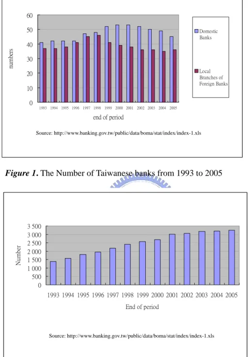
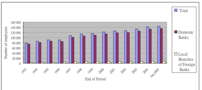
(9) competitiveness of domestic banks in Taiwan by grouping up larger Financial Holding Company (FHC). The performance of the banking sector is always an interesting topic, no matter to academicians or to governments. The main issue in measuring performance of banks includes operating efficiency, marketability, quality issues and others (Xueming Luo (2003), Lawrence M. Seiford and Joe Zhu (1999), Raman et al. (2002)). Based on the abundant literature, policy makers can make better strategic decisions for banks. However, a few issues are less addressed such as the compared efficiency of bank subsidiaries in FHCs and their competitors which we investigate in this paper. 1.2 INTRODUCTION OF THE PRESENT TAIWANESE BANKING MARKET Before we start to analyze the performance of banks, we should consider the competition and services situation in the Taiwanese banking industry from the point of view of the number of banks, employees and asset structures. According to the financial statistic data prepared by the Banking Bureau in Taiwan, there were 41 domestic banks and 37 local branches of foreign banks in 1993. There are 45 domestic banks and 36 local branches of foreign banks in 2005 as shown in Figure 11, We can observe the rapidly increasing number of banks (head office) from 1996. The overall number has reduced since 2000. Second, as shown in Figure 22, the number of domestic bank branches has increased since 2002. Since then, the intensifying of competition among Taiwanese banks has become a distinguishing feature among developing countries. Third, there are more than 140 thousand employees served in Taiwanese banks in 2005 and this is an increasing trend from 1990 as shown in Figure 3. Finally, as shown in Appendix 2, the size of the banks has become bigger and the operation is more leveraged.. 1 2. Original data as shown in Appendix 1 Refer to Appendix 1.. 2.

(10) 60 50. Domestic Banks. numbers. 40 30 Local Branches of Foreign Banks. 20 10 0. 1993 1994 1995 1996 1997 1998 1999 2000 2001 2002 2003 2004 2005. end of period Source: http://www.banking.gov.tw/public/data/boma/stat/index/index-1.xls. Number. Figure 1. The Number of Taiwanese banks from 1993 to 2005. 3 500 3 000 2 500 2 000 1 500 1 000 500 0 1993 1994 1995 1996 1997 1998 1999 2000 2001 2002 2003 2004 2005 End of period. Source: http://www.banking.gov.tw/public/data/boma/stat/index/index-1.xls. Figure 2. The Number of Taiwanese Domestic Bank Branches from 1993 to 2005. 3.

(11) Total. Number of employees. 160 000 140 000. Domestic Banks. 120 000 100 000 80 000 60 000 40 000 20 000. Ju n.2 00 5. End of Period. 20 04. 20 03. 20 02. 20 01. 20 00. 19 99. 19 98. 19 97. 19 96. 19 95. 19 94. 19 93. 0. Local Branches of Foreign Banks. Source: http://www.banking.gov.tw/public/data/boma/stat/index/index-12.xls. Figure 3. The Number of Employees Served in Taiwanese Banks from 1993 to Jun.2005 1.3 RESEARCH QUESTIONS As mentioned earlier, to go along with the Taiwanese government’ opening up of the banking market, the number of financial institutions has increased yearly, once touched the number 48, but the profit margins of banks have become thinner. In order to improve the competitiveness and efficiency of banks, it has allowed the establishment of Financial Holding Companies, which include banks, insurance firms and security brokerages in one company, since the Financial Holding Company Act was passed in 2001. It is thought that the performance of a bank subsidiary in a Financial Holding Company (FHC) is better than the independent bank, because FHC develops cross-selling strategy and provides a one-stop shopping convenience for its bank subsidiary’s customers. In fact, laws similar to the Financial Holding Company Act passed in some developed countries for the purpose of improving efficiency of financial institutions, like in the U.S. In 1999 (Gramm-Leach-Bliley Act of 1999), Canada in 1992 and United Kingdom in 1980s. Meir kohn (2004) have mentioned that as a FHC, it does reap benefits in businesses from economies of scope. For example, having securities subsidiaries to offer full-service brokerage services in an insurance firm helps an insurance company handle products such as variable annuities and mutual funds. Having banks subsidiaries helps an insurance company to save the marketing costs which is a significant part of the cost of insurance. (p.253) To encourage consolidations among different financial institutions, authorities claimed. 4.

(12) that the bank subsidiary of a FHC may outperform an independent bank, because it owns many competitive advantages compared to an independent bank, including cross-selling strategy, marketing cost savings and richer resources. Therefore, the purpose of this research is to determine whether a bank subsidiary in a FHC or independent bank has a greater efficiency and to discover whether different main businesses (banking, insurance, security) of a FHC affect the performance of its bank subsidiary. 1.4 FRAMEWORK OF ANALYSIS The rest of this thesis is organized as follows: Chapter Two: Literature Review We summarize and describe literature and techniques about two performance approaches which were used in our model briefly, including DEA approaches and Ratio Analysis. We also summarize several literature references about financial holding company, financial conglomerates and universal banks. Chapter Three: Methodologies In section one, we describe the models used in this thesis including the conventional CCR Output-oriented model ( Charnes, Cooper and Rhodes 1978), the model incorporated CCR Output-oriented model with ratio(Lovell, Pastor and Turner (1995), Lovell (1995)) and context-dependent data envelopment analysis with attractiveness and progress( Seiford and J Zhu (2003). Choice of inputs and output, selection of DMUs and adjustment of data also are described in this chapter. Chapter Four: Empirical Results We applied the techniques described in Chapter Three to calculate technical efficiency values for the banks assessed. In addition, this thesis measures context-dependent bank performance for different efficiency levels. This context-dependent DEA model allows (1) benchmarking for our Decision-Making units (DMUs) against its competitors; (2) measuring attractiveness and progress and drawing a benchmark-learning roadmap as a tool for ranking all DMUs. Chapter Five: Concluding Remarks, Limitations and Future Suggestions Summarize the empirical results and bring up some suggestions for future research.. 5.

(13) CHAPTER TWO LITERATURE REVIEW. 2.1 PERFORMANCE MEASUREMENT APPROACHES IN BANKING Performance measurement is always the main focus beyond managers. According to literature, banks have usually engaged in two kinds of measuring approaches, including Ratio Analysis and Frontier Efficiency Methodologies. We only describe Ratio Analysis and Data Envelopment Analysis (DEA), which is one of the Frontier Efficiency Methodologies, in this section, because we use a technique which incorporated DEA and Ratio Analysis to solve the research questions 2.1.1 Ratio Analysis Ratio Analysis is a traditional but popular (in practice) performance evaluating method because of its simplicity and ease of understanding. However, it suffers from three main defects. First, this analysis assumes comparable units, which implies constant returns-to-scale ( J.C. Paradi 2004). This method fails to examine whether banks operates under increasing returns-to-scale or decreasing returns-to-scale, so the banker can’t obtain early-warnings about over-invested problems. Second, each of the indicators yields a one-dimensional measure by examining only a part of the organization’s activities, or combining the multiple dimensions into a single, unsatisfactory number. (J.C. Paradi 2004) Third, financial ratios can be extracted from financial data, but they may conclude some conflicting, contradictory or confusing explanations while we consider each indicator simultaneously. Note that although ratio analysis has many detractors, the overall ease in calculations and understanding makes it maintain its unduplicated position in performance evaluation. This is in contrast to some of the frontier efficiency methodologies like the DEA technique which is treated as a black box in practice. Therefore, we include these financial ratios into our DEA assessment model and try to explain the evaluated results by financial ratios. 2.1.2 Data Envelopment Analysis Four usual Frontier Efficiency Methodology Approaches can be found in literature, including the Stochastic Frontier Approach (SFA), the Distribution-Free Approach (DFA), the. 6.

(14) Thick Frontier Approach (TFA) and the Data Envelopment Analysis (DEA)1. The Data Envelopment Analysis (hereafter DEA), one of the non-parametric methods to measure performance, is employed to assess the comparative efficiency of homogeneous operating units (this can also be called the units of assessment or Decision-Marking Units). There are abundant DEA studies about the banking industry, including the Journal of Econometrics, Journal of Banking and Finance, The European Journal of Operations research, the Journal of Economics and Business, INTERFACES, Omega and Management Science. Some of the Journals also have issued special issues about DEA, like the European Journal of Operations research. The DEA method was first described by Charnes, Cooper and Rhodes in 1978 which measures the technical efficiency frontier based the idea of Pareto optimum. Banker, Charnes and Cooper developed a revised model, called the BCC model, to measure the pure technical efficiency and scale efficiency in 1984. DEA is a linear programming formulation that defines a relationship between multiple output and inputs. It distinguishes the most efficient decision-making unit (DMU) from all DMUs. In other words, we examine the performance of each DMUs through comparing itself against Pareto-optimal peer unit (the most efficient decision-making unit). DEA is first described by Charnes et al. (1978) to evaluate the efficiency/productivity of non-profit organizations. After Sherman and Gold (1985) first adopted DEA to the banking sector, more and more financial articles have used the DEA technique to measure performance of banks and of other financial institutes. In general, researchers have evaluated banks’ and their branches’ performance from aspects of different time periods, size classes, input-output specifications and frontier techniques. Some of them have incorporated Tobit regression to explain the efficiency value; in other hand, also can use Malmquist and Window analysis to handle multiple years’ data. According to the different topics, applications can be divided into several categories as below and we review some articles employed DEA and summarized the input-output choices in Table 1. 1.. Deregulation Some economists believe that without the government policy’s interference, the market mechanism will function well by itself. However, noninterference is hard for government policy makers when considering the crucial status of the banking. 1. We also can classify performance evaluating methods into two groups: parametric and nonparametric approaches. Ratio Analysis and DEA are categorized into nonparametric approaches. SFA, DFA and TFA are categorized into parametric approaches.. 7.

(15) industry to macroeconomic and microeconomic concerns for a country. Therefore, regulations usually bind the banking sector in business scope and their operation and many researchers like to investigate the influences of government policies to efficiency/ productivity of banks and what we can predict is the negative relationships between regulations and efficiency. For these reasons, when deregulation is considered, we would like to know that is it exactly good to financial institutions. Consequently, there are many articles which discuss this topic which have been brought out. ( Berg et al.( 1992), Elyasiani and Mehdian (1995), Eukuyama (1995) Zaim (1995)) 2. Merger Many articles have tried to find out evidence to support the theory if mergers really facilitate good performance of banks or bring up abnormal returns to investors. Theodor Kohers et al. (2000) tried to find out: (1) Is the target banks’ efficiency reflected in the bidder banks’ abnormal returns? (2) Does the difference in efficiency between the bidder and target banks related to their peers influence the acquirer’s anomaly returns? Theodor Kohers et al. (2000) have successfully verified Inefficient Management Hypothesis and Low Efficiency Hypothesis by using both SFA and DEA approaches. Marcia J. Staff, et al. (1986) summarized the evolvement of. the. American Financial Act and has confirmed that a merger can’t bring abnormal returns to the bidder’s investors by regression technique. 3. Determining factors of performance: ownership, size….etc. Tser-Yieth Chen (2000) incorporated efficiency measurement with the ownership topic and found that public-owned banks perform worse in technical efficiency. Muhammet Mercan et al. (2003) have evaluated efficiency/productivity of Turkish banks for the years 1989-1999. There are some conclusions: (1) foreigner owned banks operated more efficiently than government owned; (2) size does matter. Xueming Luo (2003) employed the DEA method to measure 245 American large banks with assets in excess of 1 billion dollars, which come from the Compustat Disk, in the year 2000.. There are three conclusions. First, large banks perform better in. profitability than in marketability. Second, no evidence supports if the geographical locations of banks affect the performance of banks. Last but not least, overall technical efficiency of the profitability performance can predict the likelihood of. 8.

(16) bank failures. Lawrence M. Seiford and Joe Zhu (1999) took 55 U.S commercial banks appearing in the Fortune 1000 (Fortune April 19, 1996) as DMUs to evaluate the efficiency values. The authors found that large banks performed better in profitability. Joe Zhu(2000) calculated the efficiency values by the DEA method of 364 companies appearing in the Fortune 500 in 1995. The author found revenue-top-ranked companies do not necessarily hold the performance-top-rankings in profitability and marketability. 4. Other Applications Anja Cielen et al. (2004) employed DEA to predict bankruptcy. Chiang Kao et al.(2004) used financial forecast data, imprecise data, to obtain early-warning information needed by financial supervision and managements of banks beforehand, with integrating imprecise data into DEA model. Authors also confirmed the exactitude of performance results by comparing with the real financial data and found out that the real efficiency values are between the low bound and high bound of forecast efficiency values. Raman et al.(2002) combined the Service-profit chain into their research model and had a conclusion that the profitability of a firm will ultimately increase when a firm improves its service quality delivered to customers because good service quality will have good effects on customer satisfaction and then indirectly have positive influence on profitability. 5. Literature Review There are some literature reviews since 1978 when the first DEA model had been developed. Seiford (1996) “Data Envelopment analysis: The Evolution of the State of the Art (1978-1995)” published in Journal of Productivity Analysis, Tavares (2002) “A Bibliography of Data Envelopment Analysis (1978-2001)”. There are also some literature reviews which summarized financial institutions like Berger et al. (1997), which surveyed 130 studies that applied frontier efficiency analysis to financial institutions in 21 countries. There were 62 applications of the DEA technique.. 9.

(17) Table 1. Studies of bank performance Author(s). Model. Units. Variables. Concluding Remarks. Necmi. DEA-CCR. 16- 19 Australian trading. Model A:. 1.. Efficiencies rose in the post-deregulation period.. Kemal. Input-oriented. banks from 1986 to 1995. Inputs: (1)interest expense, (2)non-interest. 2.. Acquiring banks are more efficient than target. Avkiran. expense. banks.. (1999). Output: (1)net interest income, (2). 3.. The Acquiring bank does not always maintain its. non-interest income. pre-merger efficiency, thus decision-makers should. Model B:. be careful when choosing target banks.. Inputs:(1)deposits, (2)staff numbers Output: (1)net loans, (2)non-interest income. Seiford and. DEA-CCR. 55 U.S commercial banks. Stage 1: profitability. Relatively large banks show better performance on. J. Zhu. DEA-BCC. who have appeared in. Inputs: (1)employees, (2)assets and equity. profitability, whereas smaller banks tend to perform. Fortune 1000 (Fortune. Output: (1)revenue, (2)profit. better on marketability.. April 19, 1996). Stage 2: marketability. (1999). Inputs: (1)revenue and (2)profit Output: (1) MV, (2)TRI, and (3)EPS. TAI-HSIN. Translog. 22 domestic Taiwanese. Inputs: (1)deposits, (2)labor. HUANG. Shadow Profit. Banks for the year of. Output: (1) investments,(2)loans. (2000). Function (2000). 1981-1995. 1.. Banks should make more loans and less investment than technically efficient banks with the same input mix.. 2.. Publicly-owned banks are technically much more efficient than private banks.. 3.. Private banks are moderately efficient in allocative efficiency than public-owned banks.. Tser-Yieth Chen and. DEA-BCC. 34 Taiwanese commercial. Inputs: (1)bank staff, (2)assets, (3)bank. 1.. Private banks outperform publicly-owned banks.. banks for the year 2000.. deposits. 2.. The poor performance in pure technical efficiency. Tsai-Lien. Output: (1)loans, (2)investments, (3). Yeh (2000). non-interest revenue. 10. causes the inefficiency of publicly-owned banks..

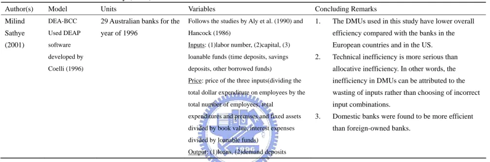
(18) Table 1. Studies of bank efficiency (cont.) Author(s). Model. Units. Variables. Concluding Remarks. Milind. DEA-BCC. 29 Australian banks for the. Follows the studies by Aly et al. (1990) and. 1.. Sathye. Used DEAP. year of 1996. Hancock (1986). efficiency compared with the banks in the. (2001). software. Inputs: (1)labor number, (2)capital, (3). European countries and in the US.. developed by. loanable funds (time deposits, savings. Coelli (1996). deposits, other borrowed funds). allocative inefficiency. In other words, the. Price: price of the three inputs(dividing the. inefficiency in DMUs can be attributed to the. total dollar expenditure on employees by the. wasting of inputs rather than choosing of incorrect. total number of employees, total. input combinations.. expenditures and premises and fixed assets divided by book value, interest expenses divided by loanable funds) Output: (1)loans, (2)demand deposits. 11. 2.. 3.. The DMUs used in this study have lower overall. Technical inefficiency is more serious than. Domestic banks were found to be more efficient than foreign-owned banks..

(19) Table 1. Studies of bank performance (cont.) Author(s). Model. Units. Variables. Concluding Remarks. Raman et. DEA-CCR. None. Model A: internal service quality efficiency. The authors suggest us to account for intangible aspects. al. (2002). Output-oriented. Inputs: (1)personnel expenses,(2)supplies,. for inputs that describe the internal service quality of. office space, (3)technology. branches into the model. Thus we can better evaluate a. Output: internal service quality survey which. bank’s performance by examining the quality of service. include four parts of questions about. delivery to external customers.. (1)market focus, (2)flexibility, (3)internal organizational efficiency and (4)empowerment. Model B: operating efficiency Inputs: (1)labor, (2)supplies, (3)office space, (4)technology and (5)account structure which include deposits, personal loans and commercial loans. Output: (1)transactions as work-output and (2)service quality, which are derived from the survey results as customer satisfaction Model C: profitability efficiency Inputs: (1)interest expenses, (2)non-interest expenses Output: (1) interest revenue, (2)non-interest revenue. 12.

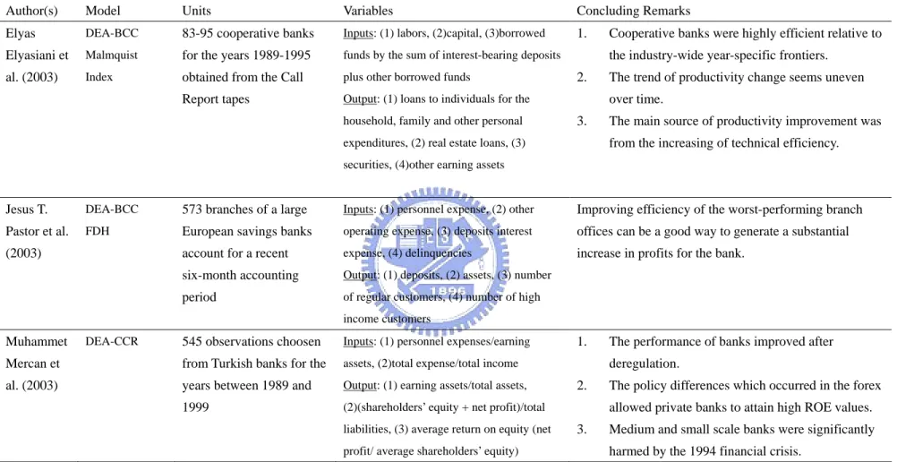
(20) Table 1. Studies of bank performance (cont.) Author(s). Model. Units. Variables. Concluding Remarks. Elyas. DEA-BCC. 83-95 cooperative banks. Inputs: (1) labors, (2)capital, (3)borrowed. 1.. Elyasiani et. Malmquist. for the years 1989-1995. funds by the sum of interest-bearing deposits. al. (2003). Index. obtained from the Call. plus other borrowed funds. Report tapes. Output: (1) loans to individuals for the household, family and other personal. Cooperative banks were highly efficient relative to the industry-wide year-specific frontiers.. 2.. The trend of productivity change seems uneven over time.. 3.. The main source of productivity improvement was from the increasing of technical efficiency.. expenditures, (2) real estate loans, (3) securities, (4)other earning assets. Jesus T.. DEA-BCC. 573 branches of a large. Inputs: (1) personnel expense, (2) other. Improving efficiency of the worst-performing branch. Pastor et al.. FDH. European savings banks. operating expense, (3) deposits interest. offices can be a good way to generate a substantial. account for a recent. expense, (4) delinquencies. increase in profits for the bank.. six-month accounting. Output: (1) deposits, (2) assets, (3) number. period. of regular customers, (4) number of high. (2003). income customers. Muhammet. 545 observations choosen. Inputs: (1) personnel expenses/earning. Mercan et. from Turkish banks for the. assets, (2)total expense/total income. al. (2003). years between 1989 and. Output: (1) earning assets/total assets,. 1999. (2)(shareholders’ equity + net profit)/total. DEA-CCR. liabilities, (3) average return on equity (net profit/ average shareholders’ equity). 13. 1.. The performance of banks improved after deregulation.. 2.. The policy differences which occurred in the forex allowed private banks to attain high ROE values.. 3.. Medium and small scale banks were significantly harmed by the 1994 financial crisis..

(21) Table 1. Studies of bank performance (cont.) Author(s). Model. Units. Variables. Concluding Remarks. Xueming. DEA-CRS. 245 American large banks. Adapted from Seiford and Zhu’s (1999). 1.. Input-oriented. with assets in excess of 1. original work.. DEA BCC. billion dollars, which. Stage1: profitability efficiency. Input-oriented. come from the Compustat. Inputs: (1) employees, (2) total assets, (3). be related to either the profitability or. Disk, in the year 2000.. equity. marketability efficiency.. Luo (2003). Lager banks perform lower efficiency in marketability.. 2.. The geographical location of banks seems to not. Output: (1) revenue and (2) profits Stage2: marketability efficiency Inputs: (1) revenue and (2) profits Output: (1) market value, (2) return to investors, and (3) EPS. Chiang. DEA- efficiency. 24. Inputs: (1) total deposits, (2) interest. The efficiency scores calculated by the data from the. Kao,. intervals (Kao. Commercial Taiwanese. expenses, (3) non-interest expenses. financial statements which were published afterwards. Shiang-Tai. and Liu (2000). banks for year 2000. Output: (1) total loans, (2) interest income,. fall into the range of predicted efficiency scores.. Liu (2004). (3) non-interest income. George E.. DEA. 15 -18 Greek commercial. Inputs: No inputs. 1.. Bigger banks show more efficiency.. Halkos et. BCC. banks members of the. Output: (1) RDIBA, (2) ROE, (3) P/L, (4). 2.. The efficiency improvement in the banking sector. al. (2004). Output–oriented. Union of Greek banks. EFF and (5) NIM. shows acompany with a reduction in the number of. from 1997-1999 Laurent Weill (2004). small banks by mergers.. DEA. Unconsolidated accounting. Inputs: (1)Personnel expenses, (2) Other non. It can be found that there is a lack of consistency in the. SFA. data for 688 banks; 135 in. interest expenses, (3) Interest paid. evaluation results among the DEA, DFA and SFA.. DFA. France, 296 in Germany,. Output: (1) Loans, (2) Investment assets. However, it has some correlation in their evaluation. 99 in Italy, 85 in Spain,. Input prices (in %): (1) Price of labor, (2). results between all frontier approaches.. and 73 in Switzerland for. Price of physical capital, (3) Price of. the years 1992-1998.. borrowed funds. 14.

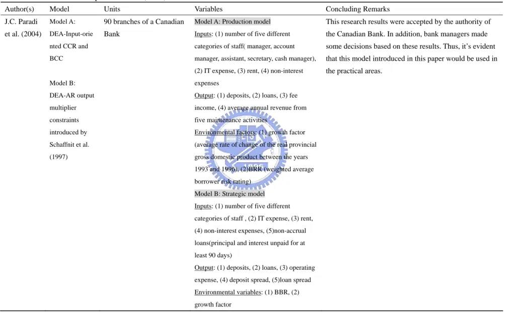
(22) Table 1. Studies of bank performance (cont.) Author(s). Model. Units. Variables. Concluding Remarks. J.C. Paradi. Model A:. 90 branches of a Canadian. Model A: Production model. This research results were accepted by the authority of. et al. (2004). DEA-Input-orie. Bank. Inputs: (1) number of five different. the Canadian Bank. In addition, bank managers made. nted CCR and. categories of staff( manager, account. some decisions based on these results. Thus, it’s evident. BCC. manager, assistant, secretary, cash manager),. that this model introduced in this paper would be used in. (2) IT expense, (3) rent, (4) non-interest. the practical areas.. Model B:. expenses. DEA-AR output. Output: (1) deposits, (2) loans, (3) fee. multiplier. income, (4) average annual revenue from. constraints. five maintenance activities. introduced by. Environmental factors: (1) growth factor. Schaffnit et al.. (average rate of change of the real provincial. (1997). gross domestic product between the years 1993 and 1996), (2)BRR (weighted average borrower risk rating) Model B: Strategic model Inputs: (1) number of five different categories of staff , (2) IT expense, (3) rent, (4) non-interest expenses, (5)non-accrual loans(principal and interest unpaid for at least 90 days) Output: (1) deposits, (2) loans, (3) operating expense, (4) deposit spread, (5)loan spread Environmental variables: (1) BBR, (2) growth factor. 15.

(23) Table 1. Studies of bank performance (cont.) Author(s). Model. Units. Variables. Concluding Remarks. TSER-YIE. DEA. 44 Taiwanese banks for. Inputs: (1) bank staff, (2) assets, (3) deposits. 1.. Input-oriented. year 1994 – 2000. Output: (1) loan services, (2) portfolio. than those found in publicly-owned banks in. investment and (3) non-interest revenue. 1994-1996.. TH CHEN. 2.. (2004). Privately-owned banks had a higher cost efficiency. Privately-owned banks had lower cost efficiency than that of publicly-owned banks in 1997-2000 when the problem of non-performing loans seems serious in privately-owned banks.. Yang Li. DFA. 40 Taiwanese banks for the. Inputs : (1) bank staff, (2) fixed assets, (3). Output-Oriented. year 1998 -2000. total deposits. their non-performing loans (NPL) as compared to. Output:(1) NPL, (2) loans, (3) portfolio. private banks.. (2004). 1.. 2.. investments. Publicly-owned banks spend more resources to cut. Compared to old banks, new banks need more resources to reduce NPL.. A.S.. DEA. 144 branches from a. Inputs: (1) number of branch and account. DEA models can provide robust estimates of cost efficiency even in situations of price uncertainty.. cone assurance. Portuguese commercial. managers, (2)number of administrative and. Camanho. regions. bank. commercial staff, (3) number of tellers, (4). et al.(2005). Input-oriented. operational costs(excluding staff cost). Output: (1) number of general service transactions. Input Prices: (1) average salary and fringe benefits of branch and account managers, (2) average salary and fringe benefits of administrative/commercial staff, (3) average salary and fringe benefits of tellers. 16.

(24) 2.2 FINANCIAL HOLDING COMPANY, FINANCIAL CONGLOMERATES AND UNIVERSAL BANKS This thesis aims to investigate whether bank subsidiaries would outperform independent banks. Therefore we review the related research first. However, we can found some similar but different terms like financial conglomerates, universal banks and financial holding companies in the research literature, thus we first state definitions of these terms. According to Fitch, Thomas P. (2002), in DICTIONARY OF BANKING TERMS, Universal Banking is “banking system in several European countries where commercial banks make loans, underwrite corporate debt, and also take equity positions in corporate securities. For example, in Germany commercial banks accept time deposits, lend money, under-write corporate stocks, and act as investment advisors to large corporations. In Germany, there has never been any separation between commercial banks and investment banks, as there is in the United States. The advantages of this type of banking system have been debated. Universal banking permits better use of customer information and allows banks to sell more services under one roof as a FINACIAL SUPERMARKET. The main disadvantage is that universal banking permits concentration of economic power to a handful of large banking institutions that hold equity positions in companies that are also borrowers of funds.” A Financial Holding Company (FHC) is a “financial entity engaged in a broad range of banking-related activities, created by the GRAMMLEACH-BLILEY ACT OF 19999. These activities include: insurance underwriting, securities dealing and underwriting, financial and investment advisory services, merchant banking, issuing or selling securitized interests in bank-eligible assets, and generally engaging in any nonbanking activity authorized by the Bank Holding Company Act.” Finally, according to Vander Vennet (2002), Financial Conglomerates are “financial institutions that offer the entire range of financial services. Next to performing the traditional banking operations, they may sell insurance, underwrite securities, and carry out security transactions on behalf of their clients.” According to the definitions, financial conglomerates and financial holding companies seem to mean the same thing; both of these. 17.

(25) two institutions serve their customers the entire range of financial services: traditional banking operations, insurance and security brokerages. On the other hand, universal bank seems providing narrow services than the other two types of financial institutes. Nowadays, many countries permit financial conglomeration including all European Union member states and the Gramm-Leach-Bliley Act of 1999 allows the establishment of Financial Holding Companies in the U.S. Since relaxing the historical barriers among traditional banking operations and other financial services like insurance and security brokerages, proponents advocate bank subsidiaries would benefit from the diversification and marketing advantages. (Arnoud W.A. Boot, 1999; Vander Vennet, 2002) However, these benefits are debated by researchers; opponents claim that there are some disadvantages in financial holding companies. For example, fewer managers’ expertise in all financial fields, thus scope diseconomies may occur. (Allen N. Berger, 2003; Bertrand Rime et al., 2003) We summarize some related literature in Table 2.. 18.

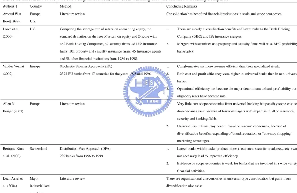
(26) Table 2. Literature review about conglomeration, universal banking and the financial holding companies Author(s). Country. Method. Concluding Remarks. Arnoud W.A.. Europe. Literature review. Consolidation has benefited financial institutions in scale and scope economies.. Boot(1999). U.S.. Lown et al.. U.S.. Comparing the average rate of return on accounting equity, the. 1.. (2000). standard deviation on the rate of return on equity and Z-score with 462 Bank holding Companies, 57 security firms, 48 Life insurance. There are clearly diversification benefits and lower risks to the Bank Holding Company (BHC) and life insurance mergers.. 2.. firms, 101 property and casualty insurance firms, 45 Insurance agents. Mergers with securities and property and casualty firms will raise BHC probability of bankruptcy.. and 58 other financial institutions from 1984 to 1998. Vander Vennet. Europe. (2002). Stochastic Frontier Approach (SFA). 1.. Conglomerates are more revenue efficient than their specialized rivals.. 2375 EU banks from 17 countries for the years 1995 and 1996. 2.. Both cost and profit efficiency were higher in universal banks than in non-universal banks.. 3.. Operational efficiency has become the major determinant to bank profitability but oligopoly rents have become rare.. Allen N.. Europe. Literature review. 1.. Berger (2003). Very little cost scope economies from universal banking but possibly some cost scope diseconomies exist because of fewer managers with expertise in all of insurance, security and banking fields.. 2.. Universal institutions may benefit from the revenue economies, because of diversification benefits, expanding of brand reputation, or “one-stop shopping” marketing advantages.. Bertrand Rime. Switzerland. et al. (2003). Distribution-Free Approach (DFA). 1.. 289 banks from 1996 to 1999. Larger banks with broader product mixes (insurance, security breakage….etc.) would not necessary lead to improved efficiency.. 2.. Evidence on scope economies is weak for banks that are involved in a wide variety of financial activities.. Dean Amel et. Major. al. (2004). industrialized. Literature review. There are organizational diseconomies in universal-type consolidation but gains from diversification also exist.. countries. 19.

(27) CHAPTER THREE METHODOLOGY. 3.1 THE TECHNIQUE Far from the first DEA model has been developed in 1978, the efficiency concept has been proposed by Farrell in 1957. Farrell (1957) proposed that the efficiency of a firm consists of two components: technical efficiency and allocative efficiency. Technical efficiency reflects the ability of a firm to obtain maximal output from a given set of inputs and allocative efficiency reflects the ability of a firm to use the inputs in optimal proportions, given their respective prices and production technology. These two measures are then combined to provide a measure of total economic efficiency. Charnes, Cooper and Rhodes (1978) (CCR models) proposed a model which had an output orientation and assumed constant returns to scale (CRS), thus technical efficiency has been discussed when using the CRS model. Later in 1984, Banker, Charnes and Cooper (BCC models) have considered both technical efficiency and allocative efficiency within a model, so we can also account for variable returns to scale (VRS) situation. The CCR and BCC models do not relate to price information and just consider input and output quantities. The choice between constant returns to scale (CRS) and variable returns to scale (VRS) is hard. Necmi K. Avkiran (2001) suggested that “ An alternative approach that removes much of the guesswork from choosing between CRS and VRS is to run the performance models under each assumption and compare the efficiency scores.” If a majority of the DMUs emerge with different scores under the two assumptions, then it is safe to assume VRS. Put another way, if the majority of DMUs are assessed as having the same efficiency, one can employ CRS without being concerned that scale inefficiency might confound the measure of technical efficiency.” By the suggestion from N.K. Avikiran (2001), we have both run BCC and CCR models and found that the majority of DMUs emerge with same efficiency scores, thus we. 20.

(28) have employed the CCR model in this thesis. In addition, we also use context-dependent DEA( Seiford and J. Zhu(2003) to rank the efficient and inefficient DMUs, and then create benchmark-learning roadmap as a tool for DMUs to realize the relative attractiveness and progress against to competitors. 3.1.1 DEA CCR model In our analysis, the efficiency measure is calculated by using the Output-Oriented version of the Charnes, Cooper and Rhodes (1978) DEA model. Assume that the objective of each DMU is to maximize its output while keeping the input level constant. Eq.(1) is the original envelopment Output-Oriented CCR DEA model, in which both inputs and output included. Unit assessed in DEA model is called DMU. Each DMU tries to maximize all their output y ,y ,………..y and maintain the level of their inputs X ,X ……X . By the 1 2. s. 1. 2. m. definition, the performance of DMU is fully (100%) efficient if and only if both θ =1 and 0. all slacks equal to zero. If smaller than 1; then we called DMU is technically inefficient. However, Eq. (1) considers both inputs and output within the model and notes that no inputs are considered in our model because we assume every DMU operated by similar and equal inputs and provide same services in the same markets thus the input constraint normally found in DEA envelopment problems is redundant (Lovell, Pastor and Turner (1995), Lovell (1995)). We then modified the conventional model as below. Considering n( set j=1,2,……n) banks which produces a matrix of output Rr (set r=1,2…,s), according Halkos et al.(2004), Lovell, Pastor and Turner (1995) and Lovell (1995), we thus can revise equation Eq.(1) to Eq.(2) which we have used to analyze the efficiency of banks assessed. A bank is efficient if and only ifθ =1 and slacks zero. 0. 21.

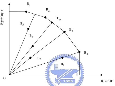
(29) Maxθ 0 s.t. n. ∑λ j =1. j. xij ≤ x, i = 1,2,.........., m. j. y rj ≥ θy r 0 , r = 1,2,......., s. n. ∑λ j =1. (1). λ j ≥ 0, j = 1,2,...., n Maxθ 0 s.t.. (2) n. ∑λ R j =1. j. rj. ≥ θ 0 Rr 0 , r = 1,2,......., s. θ 0 , λ j ≥ 0, j = 1,2,.....n Let us start to describe the DEA CCR ratio model which is used in our analysis diagrammatically. Assume that we examine the efficiency of eight commercial banks (B1, B2, B3,….B8) as shown in Figure 4; to simplify this example, we use two efficiency ratios as output: (a) R1=ROE and (b) R2=income before tax / operating revenue. In the two output CCR model solution, we draw scatter picture first; then we can find out there are four DMUs including B1, B2, B3 and B4 which achieved optimal efficiency and these four DMUs comprised efficiency frontier. We call a DMU is optimal or efficient DMU if it is on the efficiency frontier. Therefore, B5, B6, B7 and B8 are inefficient DMUs. We then can identify the efficient values by the distances between DMUs and efficiency frontier. The longer the distances are; the smaller efficient values are. The point Tµ indicates intersection of the efficiency frontier and line O Tµ. DMU located on the line O Tµ, a linear combination of B2 and B3, like B6 is with the same proportion between R2 and R3. Therefore, we call B2 and B3 as the reference set of B6 while. 22.

(30) considering performance evaluation with DEA. The efficiency value of DMU B6 is found by taking the ratio of the distances OB6/O Tµ.. R2=Margin. B1 B2 Tμ B5. B3 B6. B4 B7. B8. O R1=ROE. Figure 4. Diagrammatical DEA CCR model. 3.1.2 Context-dependent DEA One of the criticisms on CCR DEA model is its lower level of discrimination, because it only can distinguish DMUs into efficient or inefficient categories. In fact, the ranking methods have been developed to solve this lower discrimination issue. Adler et al. (2002) have divided the ranking methods into six general areas, including Cross-efficiency models, Super-efficiency model, Benchmarking, Statistics-based models, Ranking of inefficient units and multiple-criteria decision-making (MCDA/DEA)1. However, according to Adler et al. (2002), these six areas, somewhat overlapping, are useful in a specialist area but none of them can be prescribed as the complete solution to the ranking question.. 1. For a detailed description of the classification, refer to Adler et al. (2002).. 23.

(31) Some researchers have incorporated the concept “Context-Decision”, which from consumer behavior, into DEA technique to identify the efficiency differences between DMUs. Before the term” Context-Decision” has been used in the field of consumer behavior, it originated from Psychology. Psychologists said that the choice made by people would be influenced by context. Take a typical example, a small circle in a circle called circle A would make circle A look smaller; circle A surrounded with a bigger circle would make circle A look bigger. Based on this concept, Seiford and J Zhu (1996, 1999, 2003)2 suggest that context-dependent DEA can help us to differentiate relative attractiveness and progress for a particular bank from their peers. To create a benchmark-learning roadmap, we need to stratify DMUs first. We can then calculate attractiveness and progress measure values. 3.1.2.1 Stratification DEA Method Context-dependent DEA is a DEA technique to rank the efficiency of DMUs. We applied the context-dependent DEA model described by Seiford, J Zhu (2003) in this analysis. Consider a case with n(n=1,…..,j) DMUs produced a vector of output yrj=(y1j,….ysj) by using a vector of inputs xij=(x1j,…..xmj). Let J1=｛DMUj, j=1,….,n｝be the set of all n DMUs and define Jl+1=Jl-El where El= ｛DMUk ∈ Jl∣ψ*(l,k)=1｝, andψ*(l,k) is the optimal value to the following linear programming problem:. φ * (l , k ) = max φ (l , k ) λ j ,φ ( l , k ). s.t.. ∑λ. j. y j ≥ φ (l , k ) y k. ∑λ. j. x j ≤ xk. (3). j∈F ( J l ). j∈F ( J l ). λ j ≥ 0, j ∈ F ( J l ). 2. It seems that it is categorized into MCDA, according to the taxonomy by Adler et al. (2002). 24.

(32) where j ∈ F ( J l ) means DMU j ∈ J l , i.e., F (.) represents the correspondence from a DMU set to the corresponding subscript index set. When l = 1 , Eq.(3) is the original. Output-oriented CCR model, and Eq.(1) and E1 consists of the entire frontier DMUs . These DMUs in set E1 define the first-level best-practice frontier. When l = 2 , Eq.(3) gives the second-level best-practice frontier after the exclusion of the first-level frontier DMUs , and so on. By this way, we identify several levels of best-practice frontiers. We call. E l the lth-level best practice frontier. It has been mentioned in the preceding section that input constraint is redundant in our model, therefore, we amended Eq.(3) to form Eq.(4).. φ * (l , k ) = max φ (l , k ) λ j ,φ ( l , k ). s.t.. ∑λ. j. (4). y j ≥ φ (l , k ) y k. j∈F ( J l ). λ j ≥ 0, j ∈ F ( J l ) The following algorithm accomplishes the identification of these best-practice frontiers by Eq.(4). y Step 1: Set l = 1 . Evaluate the entire set of DMUs , J 1 , by Eq.(4) to obtain the. first-level frontier DMUs , set E1 ( the first-level best-practice frontier). y Step 2: Exclude the frontier DMUs from future DEA runs.. J l +1 = J l − E l . (If. J l +1 = ∅ , then stop). y Step 3: Evaluate the new subset of ‘inefficient’ DMUs , J l +1 , by Eq.(4) to obtain a. new set of efficient DMUs , E l +1 (the new best-practice frontier). y Step 4: Let l = l + 1 .. Go to step 2.. y Stopping rule: J l +1 = ∅ , the algorithm stops.. 25.

(33) 3.1.2.2 Attractiveness Measure. Based upon these evaluation contexts E l ( l = 1,…, L − 1 ), we can obtain the relative attractiveness measure by the following LP:. Ω q * (d ) = max Ω q (d ), d = 1,...L − l 0 λ j ,Ω q ( d ). s.t.. ∑λ. y j ≥ Ω q (d ) y q. ∑λ. x j ≤ xq. j j∈F ( E l 0 + d ) j j∈F ( E l 0 + d ). (5). λ j ≥ 0, j ∈ F ( E l + d ) 0. where DMUq= (xq, yq) is from a specific level E lo , lo ∈ {1, … , L − 1} .. We amended Eq. (5). to form Eq. (6) to fit our study design as mentioned previously. Ω q * (d ) = max Ω q (d ), d = 1,...L − l 0 λ j ,Ωq ( d ). s.t.. ∑λ. j j∈F ( E l 0 + d ). y j ≥ Ω q (d ) y q. (6). λ j ≥ 0, j ∈ F ( E l + d ) 0. In Eq. (6), each best-practice frontier of E lo + d represents an evaluation context for measuring the relative attractiveness of DMUs in E lo . If one DMU q owns the larger 1/ Ω q * (d) value, the more attractive the DMU q . Because this DMU q makes itself more. distinctive from the evaluation context E lo + d , we are able to rank the DMUs in E lo based upon their attractiveness scores and identify the best one.. 3.1.2.3 Progress Measure. To obtain the progress measure for a specific DMUq= (xq, yq) ∈ El0, lo ∈ {2,..., L} , we. 26.

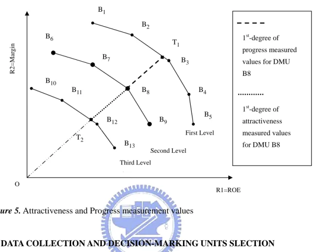
(34) use the following LP: Pq * ( g ) = max Pq ( g ), g = 1,...l 0 − 1 λ j ,Pq( g ). s.t.. ∑λ. y j ≥ Pq ( g ) y q. ∑λ. x j ≤ xq. j j∈F ( E l 0 − g ) j j∈F ( E l 0 − g ). (7). λ j ≥ 0, j ∈ F ( E l − g ) 0. As we have discussed in the preceding section, input constraint is redundant due to the design of this thesis, we amended Eq.(7) to form Eq.(8). Pq * ( g ) = max Pq ( g ), g = 1,...l 0 − 1 λ j ,Pq( g ). s.t.. ∑λ. j j∈F ( E l 0 − g ). y j ≥ Pq ( g ) y q. (8). λ j ≥ 0, j ∈ F ( E l − g ) 0. Each efficient frontier, E lo − g , contains a possible target for a specific DMU in E lo to improve its performance. The progress measure here is a level-by level improvement. For a larger Pq*(g), more progress is expected for DMU q . Thus, a smaller value of Pq*(g) is preferred. Let us start to describe the context-dependent DEA model which was developed by Seiford, J Zhu (2003) diagrammatically as shown in figure 5. Assume that we examine the efficiency for 13 commercial banks (B1, B2, B3,….B13). To simplify this example, we use two efficiency ratios: (a) R1=ROE and (b) R2=Margin (Income before Tax / Operating Revenue). We can stratify all 13 commercial banks into three levels by Eq.(4)and calculate activeness measure values and progress measure values by Eq.(6) and Eq.(8) , respectively. We can construct First Level, Second Level and Third Level efficiency frontiers by only. 27.

(35) including DMU B1, B2,…,B5 ,DMU B6,B7,..,B9 and DMU B10,B11,..,B13, , respectively. In this three levels case, we can both calculate their attractiveness and progress measure values to those DMUs in the Second Level. To DMUs in the First Level, we can only calculate attractiveness measure values. To DMUs in the Third Level, we can only calculate progress measures. We now take the B8 which in the Second Level as an example to explain how to calculate attractiveness and progress measure values. We identify the attractiveness measure values by the distances between B8 and the Third Level efficiency frontier. The distance of line OT2 is called the 1st –degree3 attractiveness measure value. Similarly, the 1st-degree progress measure values can also be measured by the distances between B8 and the First Level efficiency frontier as the distance of line OT1. The longer the distances are, the bigger are the attractiveness and progress values. As the definition, the great performers have bigger attractiveness measure values and smaller progress measure values.. 3. Note: In this three level case, 1st-degree and 2nd-degree attractiveness measured values can be calculated for First Level Context DMUs; 1st-degree attractiveness measure and 1st-degree progress measure values can be calculated for the Second Level Context DMUs; and 1st-degree and 2nd-degree progress measure values can be calculated for the Third Level Context DMUs.. 28.

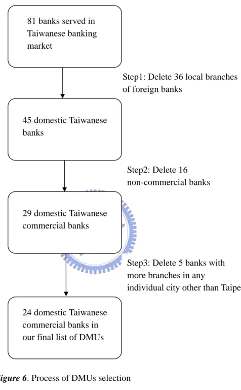
(36) B1 B2 B6. 1st-degree of. R2=Margin. T1 B7. progress measured B3. values for DMU B8. B10 B11. B8. B4. B9. B12 T2. 1st-degree of. B5. attractiveness measured values. First Level. B13. for DMU B8. Second Level. Third Level O R1=ROE. Figure 5. Attractiveness and Progress measurement values. 3.2 DATA COLLECTION AND DECISION-MARKING UNITS SLECTION. According to the Financial Statistics prepared by the Banking Bureau, Financial Supervisory Commission, Executive Yuan for the year of 20054, Taiwanese enjoy services from 45 domestic and 36 foreign bank subsidiaries, which manage over 26,875.3 billion and 2,040.5 billion ($NTD) in assets individually. 36 foreign bank subsidiaries are integrated by 15 foreign countries, including 5 from South East Asia, 4 from Japan, 2 from Hong Kong, 6 from West Europe, 6 from Middle Europe, 1 from Africa, 1 from Australia, 2 from Canada and 9 from the USA. Domestic Taiwanese banks also provide overseas services served by their overseas branches aggregating the number on a yearly basis. There were 79 overseas branches of Taiwanese banks for the year end of 2005 and they provided services in the main cities located on many countries. Homogeneity of DMUs assessed is the basic requirement while using DEA approaches.. 4. Data from website《http://www.banking.gov.tw》. 29.

(37) However, there are many differences among banks in reality including asset sizes, scopes of business, strategies focused….etc. In order to minimize the differences among our banks assessed, we designed a process to select similar banks from 45 Taiwanese banks as shown in Figure 65. As the description in Figure 6 shows, in this thesis, we focus only on commercial banking where all the products and services are similar to each other and we can ensure the homogeneity of all peer banks to satisfy the assumption of the DEA technique. Without this assumption, we can’t treat the inputs and output as comparable for all DMUs. As a result, there are 24 domestic commercial banks in our final lists of DMUs as shown in Appendix 3 and we use data from the publications of Condition and Performance of Domestic Banks for the year end of 2005 prepared by the Central Bank of China (CBC). It is noteworthy to mention that the data obtained from the Condition and Performance of Domestic Banks are collected based on unaudited figures submitted by each domestic bank’s headquarters, including the domestic banking units, offshore banking units and overseas branches, in order to publish this report on time. Thus the figures used in this thesis may differ from the information disclosed on the banks’ website which was audited by the banks or Certified Public Accountant (CPA).. 5. Non-commercial banks include two industrial banks, four business banks, one export-import banks, one commercial saving bank and other specialty banks. 5 banks with more branches in any individual city other than Taipei include the Bank Of Panhsin, Cota Bank, Luckybank, Hsinchu International Bank and Taichung Commercial Bank. To identify more similar DMUs, we limit our DMUs on those banks with headquarters in Taipei, so we can minimize the differences among DMUs. After all, banks operating in different cities may have different strategies and business scopes. Why choose Taipei? According to the Financial Statistics prepared by the Banking Bureau, Financial Supervisory Commission, Executive Yuan for the year of 2005, there are 10,223.554 billion and 6,822.296 billion NT dollars in deposits and loans provided by domestic Taiwanese banks respectively and almost half (42% and 48% of total deposits and loans) of them are concentrated in Taipei City alone. Therefore, we want to focus on those banks owning more branches located on Taipei. Moreover, this type of domestic Taiwanese banks usually have their head offices located in Taipei, except Chang Hwa Commercial Bank. Therefore, we adjusted this to limit that they should have more branches in Taipei than any other individual city.. 30.

(38) 81 banks served in Taiwanese banking market Step1: Delete 36 local branches of foreign banks 45 domestic Taiwanese banks. Step2: Delete 16 non-commercial banks 29 domestic Taiwanese commercial banks. Step3: Delete 5 banks with more branches in any individual city other than Taipei 24 domestic Taiwanese commercial banks in our final list of DMUs. Figure 6. Process of DMUs selection 3.3 SELECTION OF INPUTS AND OUTPUT 3.2.1 Choice of Inputs/Output. How to choose inputs and output when using DEA model is debated in the academic literature. The choice of inputs and output will influence the efficiency value evaluated, so we need to think thoroughly beforehand and choose the most important ones. Basically, there is a common consensus in the choice of inputs and output while calculating efficiency values. 31.

(39) employing the conventional DEA model. For example, the intermediation approach and production approach. In our paper, we choose some important financial ratio indices to capture the performances of banks assessed. 25 financial ratios, can be divided into five parts including, are Main Financial and Performance Ratios for domestic banks collected by the CBC (Central Bank of China, Taiwan) which are summarized in Appendix 4. All of these 25 indices are important but not all of them can be included into our model. We include three key factors as output to evaluate performance, which are Profitability, Asset Quality and Growth Ability, although the conventional intermediation or production approaches have not taken the measurement of risk and growth ability into account. It goes without saying of the importance of Earning Indices, so we have chosen ROE, ROA, P/L and Margin rate, all four of these are popular in practice as measurements of earning performance. Bertrand Rime et al. (2003) have mentioned that “the most obvious way to compare the performance of different size institutions is to look at familiar accounting ratios like ROA, ROE.” Muhammet Mercan et al. (2003) have used ROE as an indictor to measure the profitability. Dean Amel et al. (2002) have mentioned that “The simplest approach consists of comparing balance sheet ratios that describe costs (e.g., operating costs over gross income) and profitability (e.g., return on assets or on equity).” George E. Halkos et al. (2004) have employed ROE, P/L and ROA as profitability indicators. Hugh Crowford et al. (2004), in THE ART OF BETTER RETAIL BANKING, have mentioned that ROE is the most widely used and ROA is a common used performance measurement. In addition, the two indices are high-level and catch all measurements of performance. In fact, ROA and ROE may be treated as similar indices, however if banks are listed in order of their ROE(s), which is an approximation to a listing from best to worst, it is not the same order as their ROA(s). (p.28) Note that Margin rate is a percentage that how many net-earnings earned by firms from $100 dollar operational revenue, so we can realize the net-earning structure in operational revenue. Furthermore, the higher the Margin rate is, the more the cost efficient it is, thus to a certain extent, we can regard the Margin rate as a cost efficiency index.. 32.

(40) We can’t obtain the finest picture of a bank’s performance if we don’t include risk into consideration. In fact, authorities have focused on the risk control since 1998, because of the eruption of many crucial financial events and bankruptcy in financial sectors which were blamed to their poorer performance in risk control. In addition, authorities have given some incentives to encourage banks to reduce their Non-performing loan ratio. Therefore, we used the Non-performing loan ratio (NPL) to capture the concept of risk assessment in this paper, although NPL only captures Credit Risk of loans, not all risks faced by banks. The main reason we didn’t include all the risks is because we can’t explain those risk ratios in only one side. Take Leverage Rate as an example. According to Vasconcelos (2003), the Leverage rate expresses the institution’s ability in “circulating” more money without increasing by the same proportion its own capital, or rather, its capacity in levering assets by third party’s resources. The higher the leverage rate, the greater is the liquidity risk borne by the institution. Thus, a higher leverage rate indicates a less risk-averse institution. It is, however, more prone to insolvency if assets fall abruptly and in great numbers. By the introduction of the Leverage rate, we can understand that we can’t judge a higher leverage rate as good or bad because it may be explained by higher risk (bad) and more profit potential (good), therefore, we can’t use it as the output in the DEA model. Similar stories also happened in other risk ratios, so we don’t take them as output in our DEA model. Note that the NPL ratio is negative as related to other output values, so we should do some adjustments which will be discussed in the next section. Finally, according to (Dyson 2001) what about the so-called Target and Objectives which we have used as goals to evaluate efficiency of units of assessment usually has influenced a manager’s behaviors, and furthermore, it ultimately changes the performance of a firm. However, profitability indices are common targets for banks, although they are short-run operating outcomes. In order to make balances between long-term and short-term objectives when we measure performance of units assessed, managers should consider both long-run and short-run cases. In this thesis, we choose growth ratios of deposits and loans into. 33.

(41) our DEA model as long-run targets for banks. Note that there are four required growth ratios regulated by the CBC and we only selected two of them, since the most important and conventional activities of banks are deposits and loans businesses. Therefore we intuitively characterize banks as outstanding performers if their market share of loans and deposits are larger. In other words, the proportion of deposits and loans to the entire market and the market share of deposits and loans, can be treated as monopoly indicators. The higher of these two ratios would indicate higher profitability. The higher of the growth rate of these two ratios would indicate higher profitability prospects. As a result, we include growth rates of loans and deposits as output. In summary, we include three parts of performance measurement indices, which are asset quality, profitability and growth, and seven indicator ratios in our final list of choices of inputs and output as described below: 1.. Asset quality: Non-performing loan ratio (NPL) (%) =Non-performing loans6 divided into total loans. 2.. Profitability:. (1) Income 7-to-Average Equity (ROE) (%) (2) Income-to-Average Asset (ROA) (%) (3) Income-to- Operating Revenue (Margin) (%) (4) Income-to-number of Employee (PL) (thousand NT dollars / per employee) 3.. Growth Ability:. (1) Growth rate of Deposit (GDR) (%) (2) Growth rate of Loan (GLR) (%) 3.2.2 Examinations and Adjustments of Output Data. 6. The use of the new definition of NPLs has started from 1 July 2005. We know the old definition of NPLs before 30 June 2005 from the website of the CBC (Central Bank of China, Taiwan). According to the new definition of NPLs regulated by the CBC since 1 July 2005, the items of new NPLs’ definition includes loans which the repayment of principal or interest have been overdue for more than 3 months and any loan of which the principal debtors and surety has been disposed, although the repayment of principal or interest have not been overdue for more than 3 months. 7 Income before tax. 34.

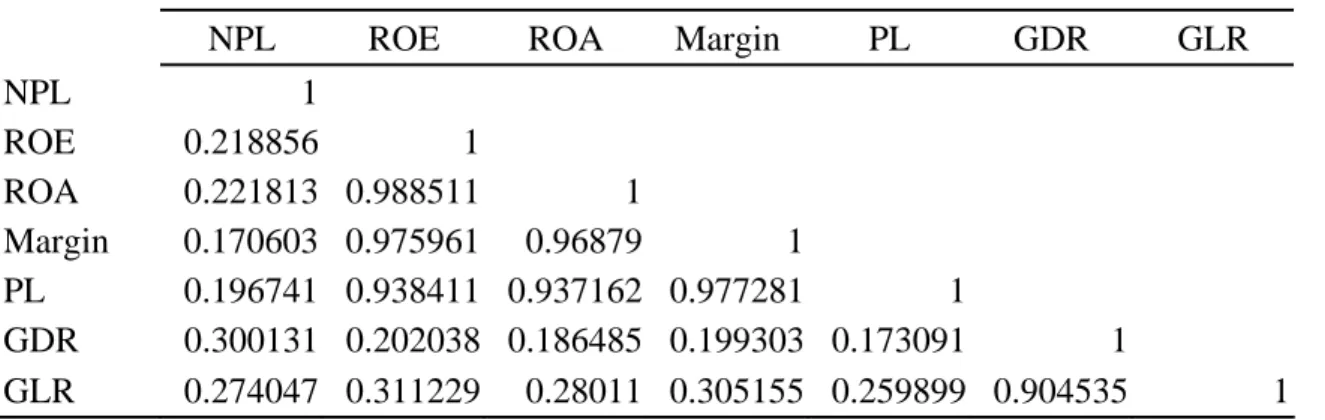
(42) The efficiency values can be easily obtained by using the DEA Excel Solver provided in Cooper, Seiford and Tone (2000). However, there are several adjustments should be done before we run the DEA Excel Solver software, when certain situations described below occur: (1) Negative values exist in data set, (2) The data set violated the basic correlation assumption required by DEA model, and this two situations can be found in our data set. Descriptive statistic of original data for year of 2005 has calculated and shown in Appendix 5. We can find out negative values and negative correlation in our output data. As shown in Appendix 5, values of ROE, ROA, Margin, PL, GDR, and GLR exit negative values, so we have paralleled the negative values to solve the negative value problem. Take ROE as an example, the parallel steps include: (1) Adding the modulus of minimum value of ROE to all ROE data; then (2) Adding one to all adjusted ROE data. There are no negative values in our data set after this adjustment process has been done. Appendix 6 is shown the coefficient correlation of the original data set for the year of 2005. It’s clearly that NPL data is negative related to all the other data, because Non-performing Loans are undesirable outputs for banks. We have done several adjustment processes by the suggestion of Seiford and J Zhu (2002, 2005): (1) Calculate the maximum value of NPL and minus all NPL to obtain a set of new data; then (2) Adding 1 to all NPL data. There are positive relationships between any of two outputs in our data set since the adjustment has been done.. 35.