A STUDY ON THE TOOL EIGENPROPERTIES OF A BTA DEEP HOLE DRILL - THEORY AND EXPERIMENTS

Pergamon Elxvier Science Ltd Printed in Great Britain OWJ-6955/9557.00 + .OO

A STUDY ON THE TOOL EIGENPROPERTIES OF A BTA

DEEP HOLE DRILL-THEORY AND EXPERIMENTS

JIH-HUA CHIN? and LI-WEI LEEt

(Received 14 July 1993; in final form 4 January 1994)

Abstract-The dynamics of a tool shaft are usually simplified to that of a second order lumped mass system for cutting process. This approach does not apply for deep hole drilling because of its extraordinary shaft length. This paper established the equations for lateral and longitudinal shaft motion of a BTA drill based on the Euler beam theory. Free-free boundary conditions are used in order to solve the eigenproperties of the shaft. Experiments to determine properties of the shaft, the shaft with internal static fluid and the shaft with cutting head were performed. The agreements between the theoretical and experimental natural frequencies and mode shapes confirmed the proposed equations. Some effects, including those of static fluid and the cutting head were clarified. This study has shown the existence and importance of the BTA tool shaft dynamics which were often overlooked or oversimplified in the past.

1. INTRODUCTION

OWING TO the extraordinary shaft length of the deep hole drill, the dynamics of the shaft itself become important to the cutting quality, so realization of shaft behavior in deep hole drilling is necessary for the operation, design and control of this machining process. Previous research into deep hole drilling has mostly discussed the relationship between cutting quality and machining conditions such as feed rate, cutting force, cutting speed and the design of the tool head or tried to find the optimum of the relationships [ 1, 2 ] but a discussion of shaft behavior was rarely provided. The dynamics of the tool shaft are usually simplified to that of a second order lumped mass system for cutting process [3]. This approach does not apply for deep hole drilling since the shaft is long enough to claim its own complex dynamics. No rigorous work has ever been carried out regarding this problem.

The purpose of this paper is to study the eigenproperties of the shaft for a BTA deep hole drill. Since the shaft behavior of deep hole drilling is coupled with the effect of pressurized fluid which is pumped into the shaft during machining, this fluid effect is also taken into consideration.

General discussions on this are found in Refs [l] and 121. Some closely related previous work is discussed as follows: Chandrashekhar et al. (1987) [4] established a three-dimensional physical model of the BTA machining system which considered the interaction between the workpiece and cutting tool. The Lagrange equations were used to obtain lateral and torsional vibration equations to represent the influence of axial force and torque. Chandrashekhar et al. [5] then found the solutions and predicted the helical grooves which were observed on the drilled workpiece and made the comparison between theoretical and experimental results. In the above papers, the shaft behaviors were not discussed. Corney and Griffiths [6] proposed the experimental analysis of the combined cutting and burnishing action in BTA drilling. El-Khabeery et al. [7] observed the surface integrity-surface roughness, hardness, micro hardness and plastic deformation of the surface under different machining conditions. Sakuma et al. [8-lo] proposed simple formulas to describe the burnishing action of guide pads and the influence on hole accuracies for different cutting force, cutting torque, depth of deformation waves on a burnished surface in BTA drilling and conducted experiments

tDepartment of Mechanical Engineering, National Chiao Tung University, Hsinchu, Taiwan, R.O.C.

30 JIH-HUA CHIN and LI-WEI LEE

to prove these theories. In their study, the relationship between cutting quality and machining conditions was studied, but shaft behavior was not considered. Sakuma et al. [8-lo] found the bending vibration of the boring bar induced by the holes corre- sponded to the number of the corners of the hole during machining. In their study, a simple model of the support and boring bar was proposed, but the influence of fluid flow was ignored.

In this paper, the shaft behavior of the BTA drill is studied and the mathematical equations for lateral and longitudinal vibration are established based upon the Bernoulli-Eulerian theory. A series of experiments are designed and performed to investigate the eigenbehavior of shaft and extensive comparisons between experimental and theoretical results are made.

2. ANALYSIS OF SHAFT DYNAMICS

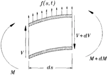
The element of the shaft is shown in Fig. 1. The equilibrium of forces yields:

V + f(s,t)d.s - (V+dV) = psA,d.s $ , (1)

where the inertia force of the element is:

The equilibrium of moments yields:

(M+dM) + f(s,t)d.r $ - (V+dV)d.s - M = 0

and

Disregarding the terms involving second powers in the equation, we obtain: av

- x + f(s,t) = psA, $ aM

- v. ds-

Substituting equation (4) into (3) gives:

V+dV i t / 1’ M+dM

(2)

(3)

(4)

a2M

as2 + psA,

as

=

a2x

and M = EI, __ _a9 so

EZ, ‘$ + p,A, >; = f(s,t).

The equation for the unforced shaft with damping can be established as follows:

(5)

3. EIGENPROPERTIES OF SHAFT WITHOUT FLUID

3.1. Lateral motion

The shaft of a BTA drill is seen as an Euler beam and the equation of motion can be written as: B.C. s = 0, a2x a3x ---_

as2 -

-=s=o

X(sJ) = 9(s) 4(t).

The mode shape function +(s) for the Euler beam is: +j(S) = COSh BjS + COS PjS - lY.j (sinh PjS + sin /3jS)

(6)

(7) and

Gosh PjI - COS pjI Oli = sinh pi1 - sin pi1

COsh pjf COS PjI = 1.

The values of Pjl are listed in Table 1.

Giving an impulse to the shaft, the equation of motion of the Euler beam becomes:

Doing the Fourier Transform of the above equation and solving for the closed form solution, we can obtain:

32 JIH-HUA CHIN and LI-WEI LEE TABLE 1. THE VALUES OF f.S,i

(coti pi1 cos pjr = 1) Pjr The values of pii

4.730040789 7.853204489 10.995607853 14.137165546 17.278759956 20.420351982 23.561944008 26.703537941 29.845129967 32.986722946 36.128316879 39.269906998

(8)

The theoretical natural frequency is equal to:

The frequency response function is:

H(ss,

sr, W) =

,zI

.

Following analysis similar to that in section 2, the equation for longitudinal motion can be obtained:

B.C.

let

es70 = 4(s) 4(t)?

the mode shape function can be obtained from the boundary condition.

(9)

BTA Deep Hole Drill

Giving an axial impulse to the shaft, the equation of motion becomes:

EA,$-p,A,$-C$=h(t).

Doing the Fourier Transform of the above equation and solving for the closed form solution, we can obtain:

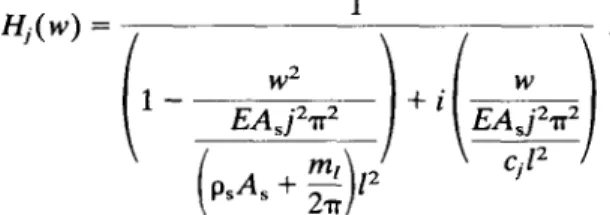
Hi(W)

W2

j2E,rr2 PSI2

(11)

The theoretical natural frequency is:

The frequency response function is:

3.3. Experiments

The arrangements of this experiment are shown in Fig. 2. The method of experiment:

(1) For lateral motion: the accelerometer is placed at point 4 and the hammer strikes the shaft from point 1 to point 15.

(2) For longitudinal motion: the hammer strikes the end of the shaft horizontally and the accelerometer is placed at points 4, 6, 8, 10 and 12.

3.3.1. Frequency response. Figures 3 and 4 show the experimental lateral and longitudinal frequency response, respectively.

3.3.2. Natural frequency.

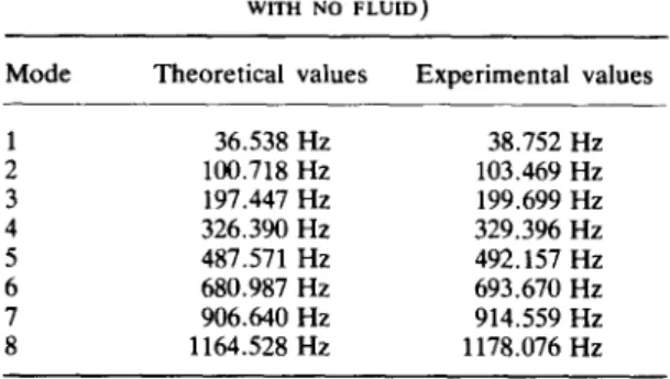
3.3.2.1. Lateral. The theoretical and experimental natural frequencies of modes l-8 are listed in Table 2 which reveals that the theoretical values of the Euler beam are close to the experimental values.

3.3.2.2. Longitudinal. Comparisons of the experimental natural frequencies of modes 1 to 3 with those of the theory are listed in Table 3. It is seen that both results stand in good agreement. 3.3.3. Mode shape. ,// “,1 ,., , ,/ Y/ H ,‘,” ,‘/j,,. .,,/

T

/,/

“‘ : / ,:

I,‘/: *,,’

;@2(*;:

34 JIH-HUA CHIN and LI-WEI LEE

HlT rmr_Fun CHa/CHl X: 693.750 Y: 495.092 curror: On

FIG. 3. The experimental frequency response for lateral vibration (shaft without fluid, B.C. free-free, measured position s = 0.4 m, exciting position s = 0.4 m).

HlTrmnsJun CHB/CHI X: 1.62Sk Y: 146.037 curror: On

FIG. 4. The experimental frequency response for longitudinal vibration (shaft without fluid, B.C. free-free, measured position s = 0.6 m, exciting position s = 0 m.

TABLE 2. THE NATURAL FREQUENCIES OF LATERAL VIBRATION OF THE SHAFC OF THE BTA DRILL (SUPPORTED HORIZONTALLY,

WITH NO FLUID)

Mode Theoretical values Experimental values 1 36.538 Hz 38.752 Hz 2 100.718 Hz 103.469 Hz 3 197.447 Hz 199.699 Hz 4 326.390 Hz 329.396 Hz 5 487.571 Hz 492.157 Hz 6 680.987 Hz 693.670 Hz 7 906.640 Hz 914.559 Hz 8 1164.528 Hz 1178.076 Hz

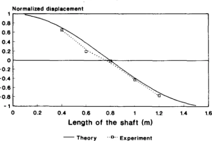
3.3.3.1. Lateral. The mode shape function of the shaft is:

+j(S) = COSh PjS + COS PjS -

CoSh @jI - COS PiI

Sinh pi, _ Sin pi/ (Sinh PjS + Sin pjS)*

TABLE 3. THE NATURAL FREQUENCIES OF LONGITUDINAL

VIBRATION OF THE SHAFT OF THE BTA DRILL (SUPPORTED HORIZONTALLY, WITH NO FLUID)

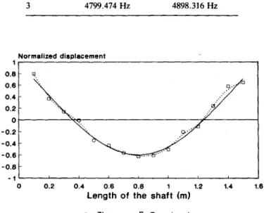
Mode Theoretical values Experimental values 1 1599.824 Hz 1615.979 Hz 2 3199.649 Hz 3255.210 Hz 3 4799.474 Hz 4898.316 Hz Normalized displacement 1 0.8 - 9 -0.2 - -0.4 - -0.6 - -0.6 - -1 0 0.2 0.4 0.6 0.6 1.2 1.4 1.6 Length of the shak (ml - Theory ‘.c.,. Experiment

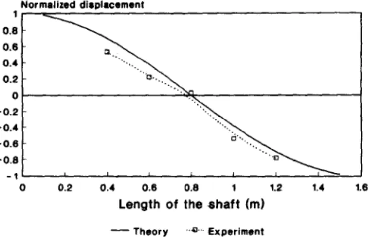
FIG. 5. The mode shape of mode 1 for lateral vibration (shaft without fluid, free-free).

experimental results are shown in Figs 5-9. It is seen that the mode shapes predicted by the theory are confirmed by experiment except the mode shape of mode 4. The reason may be that the accelerometer is placed at the node of mode 4. In the next experiment the accelerometer will be placed at point 6 to examine the results. Point 6 is a node of mode 5. It can be predicted that the mode shapes predicted by theory will be confirmed by experiments except the mode shape of mode 5 in next experiment. 3.3.3.2. Longitudinal. The mode shape function of the shaft is:

C$j(S) = COS

‘T

1

-“: :-

Length of the shalt (ml

1.2 1.4 1.6

- Theory ..w. Experiment

36 JIH-HUA CHIN and LI-WEI LEE Normalized displacement 0 0.2 0.4 0.6 0.6 1.2 1.4 1.6 Length of the shdt (m) - Theory .-a... Experiment

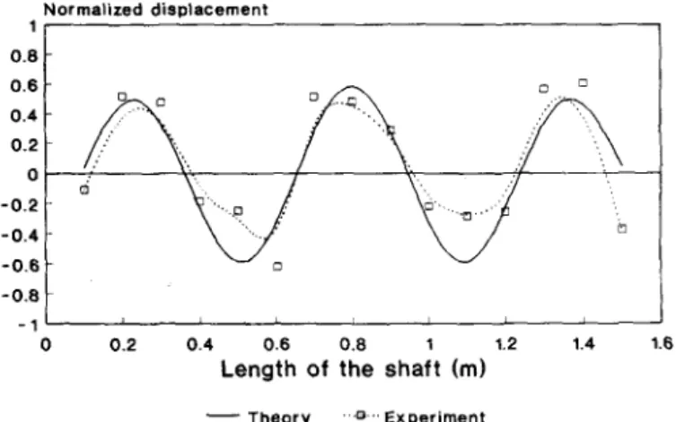
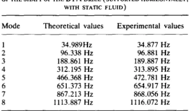
FIG. 7. The mode shape of mode 3 for lateral vibration (shaft without fluid, free-free).

Normalized displacement 1 , 0.6 0.6 - 0.4 - 0 0.2 0.4 0.6 0.8 shaflt 1.2 1.4 1.6 Length of the (m)

- Theory --e-. Experiment

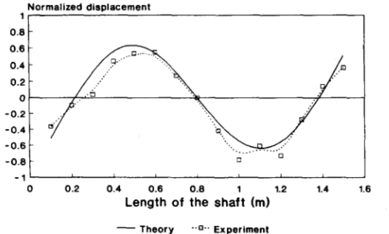
FIG. 8. The mode shape of mode 4 for lateral vibration (shaft without fluid, free-free).

Normalized displacement 0.::

-I’

0 0.2 0.4 0.6 0.8

Length of the shaflt (ml

1.2 1.4 1.6

- Theory -O-.,Experiment

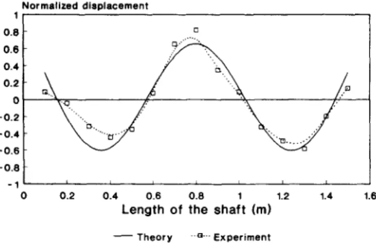
FIG. 9. The mode shape of mode 5 for lateral vibration (shaft without fluid, free-free).

The experimental mode shape of mode 1 is shown in Fig. 10. Although only five points are measured, the cosine shape can still be observed.

4. EIGENPROPERTIES OF SHAFT WITH STATIC FLUID 4.1. Lateral motion

The internal fluid influences the shaft with its mass and force (pressure) effect. Here the mass effect is examined.

BTA Deep Hole Drill Normalized dieplacemenl 0.4 - 0.2 -0.2 - -0.4 -0.8 -0.a - 0 0.2 0.4 0.6 0.8 1 1.2 1.4 1.8

Length of the shaft (ml - Theory ..a.,- Experiment

FIG. 10. The mode shape of mode 1 for longitudinal vibration (shaft without fluid, free-free).

The equation of motion of the Euler beam with static fluid:

Er, ‘$ + (p,A, + pfAf) ‘$ + Cd+ = 0

B.C.

(12)

s = 0,

a2x a3x

_s=-g=

s = I,

a*x a3x

_s=z=

the mode shape function $j(S) is the same as equation (7). Giving an impulse to the shaft, the equation of motion becomes:

EI,

‘;f +

Doing the Fourier Transform of the above equation and solving for the closed form solution, we can obtain:

The theoretical natural frequency is equal to:

38 JIH-HUA CHIN and LI-WEI LEE

The frequency response function is:

4.2. Longitudinal motion

The equation of motion:

EA, $ - (p,A, + pfAf) z - C$ = 0

B.C.

g (0,t) = 0

$

w(v) = 4(s) 4(t)

the mode shape function +j (s) is the same as equation (10). Referring to the previous section, we can obtain:

(14)

The theoretical natural frequency is:

f”=&Jz.

The frequency response function is:

4.3. Experiments

The purpose of this experiment is to examine the influence of the static fluid. The arrangements of this experiment are similar to that shown in Fig. 2 but with sealed static fluid.

The method is the same as that given in section 3.3 but with the accelerometer placed at point 6.

4.3.1. Natural frequency.

4.3.1.1. Lateral. Comparing the theoretical values of natural frequencies of modes l-8 with those of the experiment in Table 4, it is seen that the theoretical values of the Euler beam are close to the experimental values. Since the fluid term pfAf appears in the denominator within the root, the natural frequencies are expected to be lower

BTA Deep Hole Drill 39

TABLE 4. THENATURALFREQUENCIESOFLATERALVIBRATION OFTHESHAFTOFTHEBTADRILL(SUPPORTEDHORIZONTALLY,

WITH STATIC FLUID)

Mode Theoretical values Experimental values

1 34.989Hz 34.877 Hz 2 96.338 Hz 96.881 Hz 3 188.861 Hz 189.887 Hz 4 312.195 Hz 313.895 Hz 5 466.368 Hz 472.781 Hz 6 651.373 Hz 654.917 Hz 7 867.213 Hz 868.056 Hz 8 1113.887 Hz 1116.072 Hz

TABLE 5. THE NATURAL FREQUENCIES OF LONGITUDINAL VIBRATION OF THE SHAFT OF THE BTA DRILL (SUPPORTED HORIZONTALLY, WITH STATIC FLUID) (BEFORE THE EQUATION

OF MOTION BEING CORRECTED)

Mode Theoretical values Experimental values

1 1530.254 Hz 1615.979 Hz

2 3060.508 Hz 3255.210 Hz

3 4590.762 Hz 4893.316 Hz

than those of the shaft without fluid and this is indeed proven by the experimental results. This justifies the validity of the equation of motion.

4.3.1.2. Longitudinal. Comparisons of the experimental natural frequencies of modes l-3 with theoretical values are listed in Table 5. There are discrepancies, however, a check with no-fluid reveals that the fluid does not cause any change in longitudinal

2

natural frequencies. This fact can be seen from Table 6, so the term of pfAf $!$ can be neglected and the equation of motion in the longitudinal direction for this experiment can thus be modified as follows:

B.C.

a$

TABLE 6. THE EXPERIMENTAL VALUES OF THE NATURAL FREQUENCIES OF LONGITUDINAL VIBRATION OF THE SHAFT

OF THE BTA DRILL (SUPPORTED HORIZONTALLY)

Mode No fluid With static fluid

(16)

1 1615.979 Hz 1615.979 Hz

2 3255.210 Hz 3255.210 Hz

40 JIH-HUA CHIN and LI-WEI LEE

TABLET. THE NATURAL FREQUENCIES OF LONGITUDINAL VIBRATION OF THE SHAFT OF THE BTA DRILL (SUPPORTED HORIZONTALLY, WITH STATIC FLUID) (AFTER THE EQUATION

OF MOTION BEING CORRECTED AS EQUATION (16))

Mode Theoretical values Experimental values 1 1599.824 Hz 1615.979 Hz 2 3199.649 Hz 3255.210 Hz 3 4799.474 Hz 4898.316 Hz Normalized displacement 1 0.6 0.4 - 0.2

1

- _{Theory -.a.- Experiment}

FIG. 11. The mode shape of mode 1 for lateral vibration (shaft with static fluid, free-free).

The comparisons of the experimental natural frequencies of modes l-3 with those of modified theory are listed in Table 7.

4.3.2. Mode shape.

4.3.2.1. Lateral. The mode shape function of the shaft is: +j(S) = cash PjS + COS PjS - oj(sinh PUS + sin PjS)

The comparisons between the theoretical and experimental mode shapes of modes l-5 are shown in Figs 11-15. We see good agreement between the theoretical and experimental mode shapes with the exception of mode 5. This result justifies the reasoning in previous experiment.

Normalized displacement 0.6 0.4 0.2 0 -0.2 -0.4 -0.6 -0.6 0 0.2 0.4 0.6 0.8

Length of the shalt (ml

1.2 1.4 1.6

- Theory .-a-. Experiment

N o r m a l i z e d d i s p l a c e m e n t t I 0 . 8 c~ 0 . 6 c>.""". f.:

o.,o\

/...°

FIG. 13. The mode shape of mode 3 for lateral vibration (shaft with static fluid, f r e e - f r e e ) .

N o r m a l i z e d d i s p l a c e m e n t 1 0 . 8 0 . 6 0 . 4 0 . 2 0 - 0 . 2 - 0 . 4 - 0 . 6 - 0 . 8 - 1 0 E3 0 . 2 0.4 0 . 6 0 . 8 I 1.2 1.4 L e n g t h o f t h e s h a f t (m) 1.6 - - T h e o r y .-a... E x p e r i m e n t

FIt~. 14. The mode shape of mode 4 for lateral vibration (shaft with static fluid, f r e e - f r e e ) .

N o r m a l i z e d d i s p l a c e m e n t 1 0 . 8 0 . 6 o o . 0 "-... o .: -0.2 -0.4 - 0 . 6 ~ ... D ' , .." c3 . - " - 0 . 8 o - 1 I I L I I i I 0 0.2 0 . 4 0.6 0 . 8 I 1.2 1.4 1.6 L e n g t h o f t h e s h a f t (m) - - T h e o r y " ' ~ E x p e r i m e n t

Fro. 15. The mode shape o f mode 5 for lateral vibration (shaft with static fluid, f r e e - f r e e ) .

4.3.2.2.

Longitudinal.

42 JIH-HUA CHIN and LI-WEI LEE

The experimental mode shape of mode 1 is shown in Fig. 16. Again the cosine shape can be roughly seen from the five points of measurement.

5. EIGENPROPERTIES OF SHAFT WITH TOOL HEAD BUT WITHOUT FLUID

5.1. Lateral motion

The cutting head is a concentrated mass on one end of the shaft. Its influence is examined.

The equation of motion:

B.C.

s = 0, a*x a3x p-0

asZ -

s = 1, a*x --=O,E&$=m,$. _as2

The above system can be substituted by the following equivalent system:

B.C.

(17)

(18)

s = 0,

a*x

_g+Jg=o

a*x a3x

s=l, -=as’=O _as*

let

mo =

WI 4(t)

the mode shape function +j(s) is the same as equation (7).

Normalized displacement 0.4 - 0.2 o- -0.2 -0.4 -0.6 - -0.8 0 0.2 0.4 0.6 0.0 1 1.2 1.4 1.6

Length of the shaft (m) - Theory .a.. Experiment

BTA Deep Hole Drill 43 Giving an impulse to the shaft, the equation of motion becomes:

04X 02X OX 02X

EI~ ~ s 4 + p~A~ ~ - ~ + C ~ + m r S ( s - l ) ~ = h ( t ) .

Doing the Fourier Transform of the above equation and solving for the closed form solution, we can obtain:

1

H i ( w ) = . (19)

m~ j - cj - p~A~ +

2,r

The theoretical natural frequency is equal to:

= 1 /

~Elsmt.

f~ ~ psA~ + 2-- ~

The frequency response function is: M

n(Ss, Sr, W) = E ~/(Ss) IJ#](Sr) H i ( w ) . j=l

5.2. L o n g i t u d i n a l m o t i o n

The equation of motion:

02w 02w - C 0w = 0.

EA~ ~ s z - (o~A~ + pfAf) ~ - Ot (20)

B.C. O__w_w (0,t) = 0 Os 02w E A Ow (l,t) = - m I . Os Ot 2

Rearranging the above equation yields:

_ 02w O2w - A 02w - COW m t ~ ( s - l ) = O.

₍₂₁₎

44

let

JIH-HUA CHIN and LI-WEI LEE

es4 = Q(s) q(t),

the mode shape function +i(s) is the same as equation (10). Giving an axial impulse to the shaft, the equation of motion becomes:

EA, $ - psA, $ - C $ - ma(s-l) 2 = h(t).

Doing the Fourier Transform of the above equation gives:

(22)

The theoretical natural frequency is:

The frequency response function is:

5.3. Experiments

The arrangements of this experiment are similar to that shown in Fig. 2 but with tool head installed. The method is the same as that described in section 4.3.

5.3.1. Natural frequency.

5.3.1.1. Lateral. The decreases of the natural frequencies due to the tool head can be predicted by the equation of theoretical natural frequency. Comparing the theoretical values of the natural frequencies of modes l-7 with those of the experiment in Table 8, we can find the theoretical values of natural frequencies close to the experimental values and the above prediction can be proven by experimental results. Thus the equation of motion is justified.

TABLE 8. THE NATURAL FREQUENCIES OF LATERAL VIBRATION OF THE SHAI?I OF THE BTA DRILL WITH TOOL HEAD (SUP-

PORTED HORIZONTALLY, WITH NO FLUID) Mode Theoretical values Experimental values

1 35.662 Hz 35.801 Hz 2 98.305 Hz 98.048 Hz 3 192.718 Hz 185.624 Hz 4 318.572 Hz 318.327 Hz 5 475.892 Hz 480.531 Hz 6 664.675 Hz 666.543 Hz 7 884.923 Hz 868.056 Hz

TABLE 9. THE NATURAL FREQUENCIES OF LATERAL VIBRATION OF THE SHAFI OF THE BTA WITH TOOL HEAD (SUPPORTED

HORIZONTALLY, WITH NO FLUID)

Mode Theoretical values Experimental values 1 1561.504 Hz 1592.728 Hz Normalized displacement l( 0.6 - 0.6 - 0.4 - 0.2 -0.6 -

-11

FIG. 17. The mode shape of mode 1 for lateral vibration (shaft with tool head but without fluid, free-free).

5.3.1.2. Longitudinal. The comparison between the experimental and the theoretical natural frequency of mode 1 is listed in Table 9. We see good agreement between both results.

5.3.2. Mode shape.

5.3.2.1. Lateral. The mode shape function of the shaft is:

Plotting the mode shapes of modes l-5 according to the above equation and compar- ing with the experimental results given in Figs 17-21, we find that the theoretical and experimental mode shapes are in good agreement except that of mode 3. This differs from the results in the previous section. Apparently, the position of the nodes of modes 3 and 5 are shifted when the tool head is added to the shaft end.

Normalized displacement 0.: 1.1

0.6 -

0 0.2 0.4 0.6 0.6 shalt 1.2 1.4 1.6

Length of the (ml

JIH-HUA CHIN and LI-WEI LEE Normalized displacement ‘I 0.8 0 0.2 0.4 0.6 0.6 1.2 1.4 1.8 Length of the shit (m) - Theoty -a .. Experiment

FIG. 19. The mode shape of mode 3 for lateral vibration (shaft with tool head but without fluid, free-free).

Normalized displacement l- 0.8 - 0.6 - 0 0 0.2 0.4 0.6 0.8 1.2 1.4 1.6 Length of the shaflt (m) - Theory ..Q .. Experiment

FIG. 20. The mode shape of mode 4 for lateral vibration (shaft with tool head but without fluid, free-free).

FIG. 5.3.

-11

21. The mode shape of mode 5 for lateral vibration (shaft with tool head but without

2.2. Longitudinal. The mode shape function of the shaft is:

fluid, free-free).

-0.4 - -0.6 -0.6 -1 0 0.2 “.... 0.4 0.6 0.8 1 1.2 1.4 1.6

Length of the shaft (ml - Theory a.. Experiment

FIG. 22. The mode shape of mode 1 for longitudinal vibration (shaft with tool head but without fluid, free-free).

TABLE 10. THE EXPERIMENTAL NATURAL FREQUENCIES OF LATERAL VIBRATION OF THE SHAFT OF THE BTA DRILL UNDER DIFFERENT CONDITIONS

Mode No fluid With static fluid

Equipped with tool head 1 38.752 Hz 34.887 Hz 35.801 Hz 2 103.469 Hz 96.881 Hz 98.048 Hz 3 199.699 Hz 189.887 Hz 195.524 Hz 4 326.396 Hz 313.875 Hz 318.327 Hz 5 492.157 Hz 472.781 Hz 480.531 Hz 6 693.670 Hz 654.917 Hz 666.543 Hz 7 914.559 Hz 868.056 Hz 871.931 Hz

The experimental mode shape of mode 1 is shown in Fig. 22.

The comparisons of the experimental natural frequencies of the above three con- ditions of lateral vibration are shown in Table 10. We find that the conditions of the shaft with static fluid and the shaft equipped with the tool head but without fluid will reduce the natural frequencies of the shaft in the lateral direction. The effect of static fluid is more obvious than that of the tool head.

6. RESULTS AND DISCUSSION

The above investigation treats the BTA drill as a continuous beam to study its dynamics. The following conclusions can be made.

(1) There are at least seven lateral motion modes under 1000 Hz. These are far lower than those of other cutting tools. For example, Tlusty [ll] cited a long end mill with a first mode at 1400 Hz and a short end mill with a first mode at 3500 Hz. The internal cutting fluid and the tool head at the front end further reduce the natural frequencies from several Hz for mode 1 to approx. 50 Hz for mode 7. A look at Table 11 reveals that the amplitude of the lowest two modes are significant enough to influence the drilling process of which the depth of cut is in the order of millimetres.

TABLE 11. THE MAXIMAL EMPIRICAL AMPLITUDE OF MOTION (TOOL LENGTH: 1600 mm) UNIT: mm

Lateral mode Longitudinal

Mode 1 Mode 2 Mode 3 Mode 4 Mode 5 mode 1

No fluid 1.032 2.762 0.101 0.283 0.148 0.018

With fluid 4.687 1.220 0.612 1.593 0.538 0.024

48 JIH-HUA CHIN and LI-WEI LEE

(2) Lateral motion shows better agreement between theoretical and experimental results than longitudinal motion. This may be due to the fact that there are 15 striking points and five measuring points available for lateral experiment but only one striking point, the shaft end, and five measuring points available for longitudinal experiment. Further measuring points could improve the results of longitudinal experiment but each measuring point is a ground sensor seat which, when amply prepared, might change the characteristics of the tool shaft.

(3) However, the results concerning longitudinal motion are sufficient to supply knowledge of practical significance. The natural frequencies of the first longitudinal mode are higher than at least 1590 Hz and the maximal magnitude of deflection is negligible (Table 11). It was also found that the internal fluid has no effect in the longitudinal direction. This means the longitudinal motion of the tool can be neglected. The penetration effect and hence the resultant process damping may not be significant for the cutting process.

(4) Some differences between the theoretical and experimental shaft mode shape which are mainly at amplitude peaks can be seen in Figs 6 and 9. These may be caused by the suspension hindrance. Since the ideal suspension string should be very soft to allow a genuine ‘free’ motion of the shaft, this cannot be guaranteed by the actual suspension string. The deviation becomes somewhat larger in the case of a shaft with internal fluid (Figs 11-14). This is evidence that the internal fluid is not an integral part of the shaft during motion.

(5) There are significant discrepancies between theoretical and experimental mode shapes in Figs 8 and 15; examination shows that the location of the accelerometer is near the node of mode 4 in Fig. 8 and mode 5 in Fig. 15. Accelerometer seats are prepared at 0.4, 0.6, 0.8, 1.0 and 1.2 m along the tool shaft, among which 0.8 m incidentally corresponds to the node of mode 2; 0.4, 0.8 and 1.2 m correspond to the node of mode 4; while 0.6 and 1.0 m are near the node of mode 5. If the accelerometer seats were prepared at places other than the nodes of all possible motion modes, better agreement could be expected. On the contrary, the suspension strings should be fixed on the node to reduce possible suspension hindrance. In addition, the mass of the accelerometer should be as small as possible. There is an accelerometer with 0.1 g mass, but which is not available owing to an international export regulation.

(6) The tool head can be treated as a concentrated mass on the shaft end. Its influence is less than that of the internal fluid, but it causes the mode shape to be less symmetrical. The head side becomes more reluctant in dynamics and the nodes of mode 3 are shifted (compare Figs 19 and 7). Since the disposition of the cutting lips are not symmetrical, the asymmetric cutting force might amplify this effect to give a complicated head motion.

7. CONCLUSIONS

The shaft of a BTA deep hole drill is long enough to claim its own dynamics which may influence the cutting process taking place at the tool head. This effect has not been rigorously studied in the past. This paper established the equations for lateral and longitudinal motion based on the Euler beam theory. Effects of the cutting head and internal fluid were included. Solutions were found for free-free boundary conditions. Theoretical natural frequencies and mode shapes were obtained. Three series of exper- iments were performed. Satisfactory agreements between theoretical and experimental results confirmed the validity of the Euler beam approach and the proposed equations. In addition, the studies reveal the following facts: (1) the lateral natural frequencies are far lower than the longitudinal natural frquencies. This means that the lateral vibrational behavior of the shaft is most likely to influence the cutting process; (2) the longitudinal natural frequencies are not influenced by the static internal fluid. Since their natural frequencies are almost over 1600 Hz, the longitudinal vibrational behaviors may have little influence upon the cutting process; (3) the mass effect of internal fluid on the lateral natural frequencies is slightly larger than the effect of the cutting head.

However, the pressure effect of the internal fluid is not covered in this study. This remains to be examined in the future; and (4) the cutting head may shift the node position of the shaft mode shape.

Acknowledgement-This research was supported by the National Science Council of the Republic of China under Grant No. NSC-82-0401-E-009-140.

REFERENCES

[l] J.-H. CHIN, J.-S. Wu and R. S. YOUNG, The computer simulation and experimental analysis of chip monitoring for deep hole drilling, ASME J. Engng Znd. 115, 184-192 (1993).

[2 ]B. J. GRIFFITHS, Modelling complex force systems, Part 1: The cutting and pad forces in deep drilling,

ASME J. Engng Ind. 115, 169-176 (1993).

[3] F. ISMAIL, M. A. ELBESTAWI, R. Du and K. URBASIK, Generation of milled surfaces including tool dynamics and wear, ASME J. Engng Ind. 115, 245-252 (1993).

[4] S. CHANDRASHEKHAR, T. S. SANKAR and M. 0. M. OSMAN, A stochastic characterization of the machine tool workpiece system in BTA deep hole machining-Part I. Mathematical modelling and analysis, Adv. Manufact. Processes, 2(1/2), 37-69 (1987).

[5] S. CHANDRASHEKHAR, T. S. SANKAR and M. 0. M. OSMAN, A stochastic characterization of the machine tool workpiece system in BTA deep hole machining-Part II. Response analysis and evaluation of the tool tip motion, Adv. Manufact. Processes, 2(1/2), 71-104 (1987).

(61 J. CORNEY and B. GRIFFITHS, A study of the cutting and burnishing operation during deep hole drilling and its relationship to drill wear, Znr. J. Prod. Res. 14, l-9 (1976).

[7] M. M. EL-KHABEERY, S. M. SALEH and M. R. RAMADAN, Some observations of surface integrity of deep drilling holes, Wear 142, 331-349 (1991).

[8] K. SAKUMA, K. TAGUCHI and A. KATSUKI, Study on deep-hole-drilling with solid-boring tool-The burnishing action of guide pads-and their influence on hole accuracies, Bull. JSME 23, 1921-1928 (1980).

[9] K. SAKUMA, K. TAGUCHI and A. KATSUKI, Study on deep-hole boring by BTA system solid boring tool-behaviour of tool and its effect on profile of machined hole, Bull. Jpn. Sot. Prec. Engng 14, 143-148 (1980).

[lo] K. SAKUMA, K. TAGUCHI and A. KATSUKI, Self-guiding action of deep-hole-drilling tools, Ann. CIRP 30, 311-315 (1981).

[ll] J. TLUS~, Dynamics of high-speed milling, ASME J. Engng Znd. 108, 59-64 (1986). APPENDIX

The equipment used in the experiments: 1. Machine tool:

SAN SHING SK26120 heavy duty precision lathe. 2. Hammer:

Hammer: PCB 086B05 SN5163 Range: O-5000 lb

Amnlifier: PCB model 480DO6 Dower unit. 3. Accelerometer:

Accelerometer: TEAC 6012 Weight: 0.3 g

Amplifier: TEAC SA620. 4. Spectrum analyzers: Microlink and Signal Doctor

5. The Deep Hole Drill: (a) Drill head:

Type: SANDVIK 420.6-0014D 18.91 70 Mass: 0.030205 kg

Mass moment of inertia J,: 1.420 x 10e6 kg.m* (b) Drill tube: Type: SANDVIK 420.5-800-2 Length: 1.6 m Internal diameter: 11.5 mm External diameter: 17.0 mm Material: JIS SNCM 21 Density p.: 7860 kg/m3 Young’s modulus E: 2.06 x 10” Pa Shear modulus G: 8.1 x lOi Pa 6. Fluid:

Type: R68

Density pr: 866 kg/m3