一個控制細微粒及奈米微粒排放的電極線-平板型濕式靜電集塵器

(1)

國

立

交

通

大

學

環境工程研究所

博

士

論

文

一個控制細微粒及奈米微粒排放的

電極線-平板型濕式靜電集塵器

A Wire-in-Plate Wet Electrostatic Precipitator for Controlling

Fine and Nanosized Particle Emission

研究生：林冠宇

指導教授：蔡春進教授

(2)

一個控制細微粒及奈米微粒排放的

電極線-平板型濕式靜電集塵器

A Wire-in-Plate Wet Electrostatic Precipitator for Controlling

Fine and Nanosized Particle Emission

研究生：林冠宇

Student：Guan-Yu Lin

指導教授：蔡春進

Advisor：Chuen-Jinn Tsai

國立交通大學

環境工程研究所

博士論文

A thesis

Submitted to Institute of Environmental Engineering National Chiao Tung University

in Partial Fulfillment of the Requirements for the Degree of

Doctor of Philosophy in

Environmental Engineering August 2010

Hsinchu, Taiwan, Republic of China

中華民國九十九年八月

(3)

一個控制細微粒及奈米微粒排放的

電極線-平板型濕式靜電集塵器

學生：林冠宇　　　

指導教授：蔡春進

國立交通大學環境工程研究所

摘要

本研究設計並開發一個高效率電極線-平板型濕式靜電集塵器用以控制細微粒及奈米微粒污染物。本集塵器之寬為 75 mm，有效微粒沈降長度及氣膠通道間隙分別為 48 mm 及 9.0 mm。本濕式靜電集塵器之收集板表面經噴砂處理後塗敷 TiO2奈米微粒，以提高表面親水性，用以取代親水性薄膜的設計；電暈放電電極由三條黃金電極線(直徑為 100μm)所構成；一個氣體脈衝閥用以連續且規律的清潔附著在電極線表面之粉塵，使集塵器維持最佳的集塵效率。本濕式靜電集塵器之設計目的在於解決以下傳統乾式靜電集塵器在使用上之問題：粉塵沈降於收集板表面及放電電極上使集塵效率下降、背電暈及粉塵再揚起。最後，我們在起始乾淨條件下及經過高濃度粉塵負荷後進行濕式靜電集塵器集塵效率測試，並與乾式靜電集塵器之測試結果做比較。實驗結果顯示當施加電壓為4.3 kV、氣膠流量為 5 L/min（微粒停留時間為 0.39 s）時，本濕式靜電集塵器在起始乾淨狀況下對16.8-615 nm 電移動度粒徑之奈米微粒去除效率為96.9-99.7 %。在相同操作條件下經過 1.2±0.06 g/plate 之 TiO2高粉塵濃度負荷後，濕式集塵器對於16.8-615 nm 之玉米油微粒之去除效率仍可維持在 94.7-99.0 %。本研究首先建立了一個拉式數值模式來推估靜電集塵器對粒徑分佈為 0.1≦dp≦10 μm 之微粒的集塵效率。微粒的充電及運動方程式係利用四階 Runge-Kutta 法來求解，以

(4)

求得微粒的帶電量及微粒移動軌跡。比對結果發現，模擬出的收集效率與 Huang and Chen (2002)及 Chang and Bai (1999)的實驗值相符，誤差範圍分別為 0.68-14.57 %及

1.49-12.46 %。但此模式僅適用於推估靜電集塵器對 dp≧100 nm之微粒的集塵效率，無法有效計算出部分充電效應對奈米微粒收集效率的影響。為了準確預估單極電極線-平板靜電集塵器對奈米微粒(dp≦100 nm)的收集效率，本研究建立了一個2 維數值歐拉模式來模擬電場、離子濃度分佈，及微粒充電量。集塵器內部的流場係利用SIMPLER 方法來計算之，而電場強度及離子濃度分佈則利用 Poisson 方程式及對流擴散方程式來求解。帶電微粒的濃度分佈及微粒去除效率分別利用對流擴散方程式及Fuch 充電理論進行計算。

針對6-100 nm 之奈米微粒，本研究模擬之微粒收集效率與 Huang and Chen (2002)

的實驗數據比對結果發現，模擬值與實驗值吻合(氣膠流量: 100 L/min, 施加電壓: -15.5~-21.5 kV)。進一步比對模擬的收集效率值與濕式靜電集塵器(Lin et al. 2010)的收集效率實驗值結果發現，模擬值與集塵器對單徑分佈、粒徑為10 及 50 nm 的食鹽微粒及多徑分佈、粒徑分佈範圍為5.23-107.5 nm 之銀微粒的去除效率實驗值相符(氣膠流量: 5 L/min, 施加電壓: +3.6~+4.3 kV)。本單極電極線-平板型濕式靜電集塵器在高濃度粉塵負荷下可有效的去除細微粒及奈米微粒。預期本濕式靜電集塵器可作為高效率微粒去除設備及奈米微粒採樣器。本研究建立的數值模式可用於設計大型的單極平板濕式靜電集塵器，以解決傳統乾式靜電集塵器在實際操作上所面臨的問題。

(5)

A Wire-in-Plate Wet Electrostatic Precipitator for Controlling

Fine and Nanosized Particle Emission

Student: Guan-Yu Lin

Adviser:Dr. Chuen-Jinn Tsai

Institute of Environmental Engineering

National Chiao Tung University

ABSTRACT

In this study, an efficient parallel-plate single-stage wet electrostatic precipitator (wet ESP) with a width of 75 mm, effective precipitation length of 48 mm and gap of 9.0 mm was designed and tested to control fine and nanosized particles without the need of rapping. The collection plates are made of sand-blasted copper plates coated with TiO2 nanopowder instead

of hydrophilic membranes. Three gold wires (diameter: 100 µm) were used as the discharge electrodes and a pulse jet valve was used to regularly purge the wires. The design of the present wet ESP is aimed at solving the problems of traditional dry ESPs: reduction of the collection efficiency due to particle deposition on the discharge electrodes and collection electrodes, back corona, and particle re-entrainment. The collection efficiency at initially clean and heavy particle loading conditions was tested and compared to a similar dry ESP.

Experimental results showed that when the wet ESP was initially clean, the particle collection efficiency ranged from 96.9-99.7% for particles ranging from 16.8 to 615 nm in electrical mobility diameter at an aerosol flow rate of 5 L/min (residence time of 0.39 sec) and an applied voltage of 4.3 kV. After heavy loading with TiO2 nanopowder about 1.2±0.06

(6)

reduce only slightly to 94.7-99.0 % for particles from 16.8 to 615 nm in diameter.

In order to predict collection efficiency for particles with 0.1≦dp≦10 μm, a numerical

model based on Lagrangian method was developed. The equation of particle charging and particle motion were solved by using the fourth order Runge-Kutta integration to obtain particle charges and trajectory. The simulated particle collection efficiencies based on Lagrangian method were shown to agree reasonably with the experimental data in Huang and Chen (2002) and Chang and Bai (1999) with deviation of 0.68-14.57 % and 1.49-12.46 %, respectively. This model, which can’t be used to predict partial charging effect on nanoparticle collection efficiency, is appropriate to be used to predict collection efficiency of ESPs for particles with dp≧100 nm

In order to predict nanoparticle (dp≦100 nm) collection efficiency in single-stage

wire-in-plate ESPs accurately, the electric field, the ion concentration distribution, and the particle charge were obtained by a 2-D numerical model based on the Eulerian method. Laminar flow field was solved by using the Semi-Implicit Method for Pressure-Linked Equation (SIMPLER Method), while electric field strength and ion concentration distribution were solved based on Poisson and convection-diffusion equations, respectively. The charged particle concentration distribution and the particle collection efficiency were calculated based on the convection-diffusion equation with particle charging calculated by Fuchs diffusion charging theory.

The simulated collection efficiencies of 6-100 nm nanoparticles were compared with the experimental data of Huang and Chen (2002) for a wire-in-plate dry ESP (aerosol flow rate: 100 L/min, applied voltage: -15.5~-21.5 kV). Good agreement was obtained. The simulated particle collection efficiencies were further shown to agree with the experimental data obtained in the study for a wire-in-plate wet ESP (Lin et al. 2010) (aerosol flow rate: 5 L/min, applied voltage: +3.6~+4.3 kV) using monodisperse NaCl particles of 10 and 50 nm in diameter, and polydisperse Ag particles of 5.23-107.5 nm in diameter.

(7)

The present single-stage wire-in-plate wet ESP was found to remove fine and nanosized particle effectively under heavy loading conditions. It is expected that the present wet ESP could be used as efficient particle removal equipment or a nanoparticle sampler. The present model could facilitate the design and scale-up of the single-stage wire-in-plate wet ESP to control fine and nanosized particles without the typical problems associated with dry ESPs.

(8)

LIST OF TABLES

Table 2.1 Arrangement of literature reviews in experimental studies of wet ESPs. ... 14 Table 2.2 Arrangement of literature reviews in numerical studies of particle collection

efficiencies in wire-in-plate ESPs. ... 15 Table 3.1 Characteristics of the test particles ... 25 Table 4.1 Comparison of different models for particle charging by field, diffusion, and

combined charging. ... 55 Table 4.2 Ion molecular weight, ion mobility, and the corresponding ion diffusion

coefficient used in previous researches... 64 Table 4.3. Combination coefficient of positive ion with 50 and 10 nm NaCl particles

calculated by using different ion molecular weights shown in Table 1 based on Fuchs theory. ... 76 Table 4.4 Typical design parameter for ESPs (http://yosemite.epa.gov/oaqps/EOGtrain.nsf/ 83 DisplayView/SI_412A_0-5?OpenDocument)... 83

(11)

LIST OF FIGURES

Figure 3.1 Schematic diagram of the parallel-plate wet ESP. Plexiglass plates (M), enter piece (C), frosted glass plate (FG), sand-blasted copper plate (G), overflowing reservoir (OR), collecting reservoir (CR), golden wire (GW), liquid inlet (LI), liquid outlet (LO), aerosol inlet (AI), aerosol outlet (AO), pulse jet valve (PJ), air hole (AH)...17 Figure 3.2 SEM image of micromorphological characteristic of the frosted copper plate

coated with TiO2 nanopowder. (a) X 70,000, (b) X 100,000. ...20

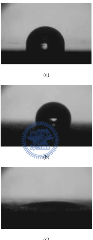
Figure 3.3 Water contact angle on three copper plate surfaces. (a) smooth surface, (b) sand-blasted surface, and (c) sand-blasted surface coated with TiO2 nanopowder.21

Figure 3.4 Experimental setup for particle collection efficiency and particle loading tests. ....26 Figure 3.5 Experimental setup for monodisperse NaCl particle collection efficiency...27 Figure 3.6 Calculation domain (a) the single-stage wire-in-plate dry ESP (Huang and Cheng

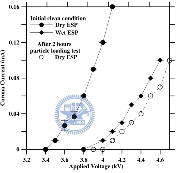
2002), (b) the single-stage wire-in-plate wet ESP (Lin et al. 2010). (unit: m)...32 Figure 4.1 Corona current as a function of applied voltage in the dry and wet ESPs. ...42 Figure 4.2 Collection efficiency of the present wet ESP for corn oil particles at the aerosol

flow rate 5 and 10 L/min and the applied voltage of 4.3 kV. Each test was repeated 6 times. ...43 Figure 4.3 Collection efficiency of the present wet ESP for corn oil particles under different

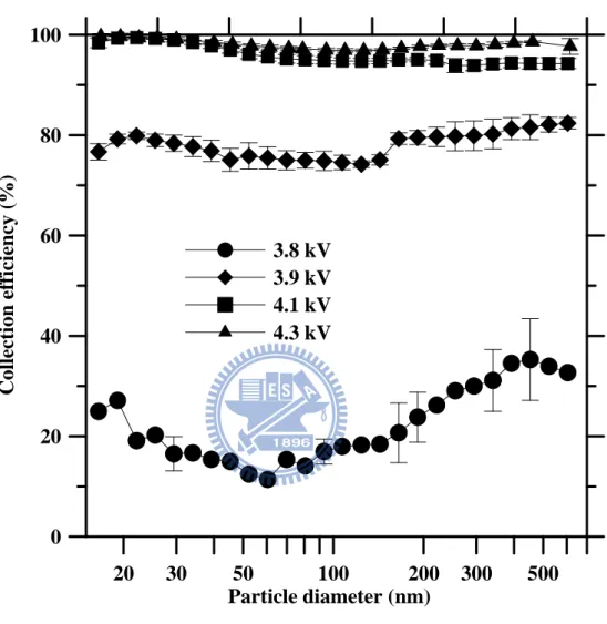
applied voltages. The aerosol flow rate is fixed at 5 L/min. Each test was repeated 6 times. ...46 Figure 4.4 Collection efficiency of the present wet ESP for corn oil particles under different

applied voltages. The aerosol flow rate is fixed at 10 L/min. Each test was repeated 6 times. ...47 Figure 4.5 Electrostatic precipitation and diffusive deposition efficiencies of the

polydisperse corn oil particles in the present wet ESP when the aerosol flow rate and the applied voltage are 5 L/min and 4.3 kV, respectively. Each test was repeated 6 times. ...48 Figure 4.6 Collection efficiency for corn oil particles in the dry ESP at different TiO2

nanopowder loadings. The applied voltage and aerosol flow rate are 4.3 kV and 5 L/min, respectively. ...51 Figure 4.7 Particle reentrainment test in dry ESPs. The aerosol flow rate and applied

voltage were 5 L/min and 4.3 kV. ...52 Figure 4.8 Collection efficiency for corn oil particles in the wet ESP at different TiO2

nanopowder loadings. The applied voltage and aerosol flow rate are 4.3 kV and 5 L/min, respectively. ...53 Figure 4.9 Comparison of the simulated particle trajectory between the present numerical

(12)

open symbol: the numerical results in Goo and Lee (1997)). ...56 Figure 4.10 Comparison of the simulated particle charging between the present numerical

results and those in Goo and Lee (1997) (Line: the present numerical results; open symbol: the numerical results in Goo and Lee (1997)). ...57 Figure 4.11 Comparison of particle collection efficiency in the single-stage wire-in-plate

dry ESP between numerical results and experimental data in Huang and Chen (2002) at the aerosol flow rate of 100 L/min...60 Figure 4.12 Comparison of particle collection efficiency in the single-stage wire-in-plate

dry ESP between numerical results and experimental data in Chang and Bai (1999) at an aerosol flow rate of 109 L/min and an applied voltage of 27.0 kV...61 Figure 4.13 Comparison of Corona current as a function of applied voltage between

theoretical results and experimental data in the ESP...65 Figure 4.14 Comparison of electric field strength and ion concentration distribution

between numerical results and analytical solutions in a wire-in-tube ESP for (a) positive ions, and (b) negative ions. ...66 Figure 4.15 Electric potential distribution at the applied voltage of +3.7 kV in the wet ESP.

(Note: The scale in y direction is magnified 4.5 times relative to that in x direction.)...67 Figure 4.16 Ion concentration distribution at the applied voltage of +3.7 kV in the wet ESP.

(Note: The scale in y direction is magnified 4.5 times relative to that in x direction.)...68 Figure 4.17 Comparison of particle collection efficiency in the single-stage wire-in-plate

dry ESP between numerical results and experimental data in Huang and Chen (2002) at the aerosol flow rate of 100 L/min...72 Figure 4.18 Number concentration distribution of 6 nm particles carrying 0 and 1 charges in

the single-stage wire-in-plate dry ESP (Huang and Chen 2002) when the applied voltage and air flow rate was -15.5 kV and 100 L/min, respectively. (a) 0 charge, (b) 1charge. ...73 Figure 4.19 Comparison of particle collection efficiency in the single-stage wire-in-plate

wet ESP between numerical results and experimental data at the air flow rate of 5 L/min. ...77 Figure 4.20 Number concentration distribution of 50 nm particles carrying 0-4 charges in

the single-stage wire-in-plate wet ESP when the applied voltage and air flow rate was +3.7 kV and 5 L/min, respectively. (a) 0 charge, (b) 1charge, (c) 4 charges. (Note: The scale in y direction is magnified 4.5 times relative to that in x direction...78 Figure 4.21 Collection efficiencies of the polydisperse silver particles in the present wet

(13)

+3.7-+3.9kV, respectively. Each test was repeated 6 times. ...80 Figure 4.22 Turbulent flow field in the simulated pilot scale wet ESP, (a) simulated result

calculated by using SIMPLER algorithm (Patankar 1980), and using (b) the CFD commercial code, Star CCM...84 Figure 4.23 Collection efficiencies of particles in the pilot scale wet ESP under different

design parameters. The applied voltage was 70 kV. ...85 Figure 4.24 Comparison of the collection efficiency for particles with 5≦dp≦100 nm in

ESPs which have 3, 6, or 9 discharge wires (diameter=2.5 mm). (a) The ESPs have 3 and 6 wires, (b) The ESP have 6 and 9 wires. ...86

(14)

LIST OF SYMBOLS

A total collection area (m2)

a radius of particles (m)

Cc Cunningham slip correction factor

CD empirical drag coefficient

Cin(dp) particle inlet concentration (cm-3)

Cout(dp) outlet concentration (cm-3) for particle of diameter dp

i

c _{mean thermal speed of the ions (m/s)} dp particle diameter (nm)

D0 turbulent dispersion coefficient within the turbulent core of the

flow (m2_/s)

DH hydraulic diameter (m)

Di diffusion coefficient of ions (m2/s)

DB Brownian diffusion coefficient of particles (m2/s)

Deddy Eddy diffusivity of a particle (m2/s)

E electric field strength (V/m)

Ec corona initiating electric field (V/m)

Eave average electric field strength (V/m)

Ex electric field strength in x direction (V/m)

Ey electric field strength in y direction (V/m)

e elementary electrical charge 1.6×10-19

f wire roughness factor fr friction factor

GIN first iterate correction to the flux 0.26.

h distance from the wall to the interface between the region of a linearly increasing dispersion coefficient and that of a constant dispersion coefficient (m)

I total current per discharge wire (A)

Jp average current density at the collection plate (A/m2)

KE constant of proportionality

Kn Knudsen number

k turbulent kinetic energy (J/s-kg)

kc constant 0.4~0.6

kb Boltzmann constant J/K 1.38×10-23

l wire length (m)

(15)

Mi molecular weights of ions (kg/mol)

Mair molecular weights of air (kg/mol)

Na Avogadro number 1/mol 6.023×1023

Ni ion number concentration (m-3)

Np,q concentration of particles carrying q elementary charges (m-3)

Np,0,total(y) inlet uncharged particle number concentration (m-3)

Np,q,outlet(y)

outlet number concentration of particles carrying q elementary charges (m-3)

P0 pressure (atm) 1 (atm)

Q air flow rate (m/s)

q number of charges carried by particles qsat saturation charge (C)

r distance between particles and ions center (m) ra apsoidal distance (m)

Re Reynolds number based on the hydraulic diameter Rep particle Reynolds number

reff equivalent cylinder radius (m)

rc wire radius (m)

Sc generation of particles with q-1 charges.

sx half wire to wire spacing (m)

sy wire to plate spacing (m)

T temperature (K)

T0 temperature (K) 293 (K)

u air velocity in x direction (m/s)

u* _{velocity distribution of a fully developed turbulent flow (m/s)}

uave average air velocity (m/s)

up particle velocity in x direction (m/s)

v air velocity in y direction (m/s) vp particle velocity in y direction (m/s)

V potential (Volt)

V0 applied voltage (kV) 3.6-4.3

Vc corona onset voltage (V)

VTE particle migration velocity (m/s)

VTE,k average migration velocity of particles (m)

Wloaded quantity of particles in the ESP per plate (g)

(16)

Wtotal total particle dispersed by the Jet-O-Mizer (g)

Wex particles in the excess flow (g)

Zi ion mobility (m2/s-V)

ZP particle electrical mobility (m2/s-V)

αq combination coefficient of ions for particles carrying q

elementary charges (m3/s)

ηtotal(dp) particle collection efficiency of the wet ESP

λion mean free path of ions (nm)

δ relative density of air

δr radius of the limiting sphere (m)

ρair air density (kg/m3)

ρc ion density at the boundary of the ionized sheath (A･sec/m-3)

ρi space charge density (C/m3)

κd dielectric constant of particle (salt) 6.2

ε turbulent dissipation rate (J/s-kg)

ε0 permittivity of free air (F/m) 8.85×10-12

ξ striking probability

ξp turbulent dispersion coefficient within the turbulent core of the

flow (m2/s)

 _{electrostatic potential between the particle and the ion} μair viscosity (kg/m-s)

(17)

CHAPTER 1 INTRODUCTION

1.1 Motivation

In recent year, the applications of nanomaterials are increasing rapidly in many industries including textile, optics, electronics, medical devices, biosensors, and environmental remediation (Smith et al. 2007). During manufacturing and shipping of nanomaterials, nanoparticles could be released into environment posing adverse effects on aquatic species and human health (Griffitt et al. 2007; Oberdörster et al. 2005). Thus, efficient control of nanoparticle emissions effectively has become an important research topic.

Electrostatic precipitators (ESPs), including dry and wet types, have been widely used to remove particles emitted from various industrial processes. ESPs are capable of handing large flow rates of exhaust gas with low electrical power consumption because of it’ low pressure drop through the collection chamber (USEPA 1999). When particles are introduced into a single-stage ESP, they are charged by diffusion and field charging mechanisms and are collected by electrostatic forces on the collection electrodes (Hinds 1999). In a well-designed dry ESP, the collection efficiency for micron and submicron particles can reach up to 95% as shown in several experimental (Huang and Chen 2002; Marek et al. 2005) and numerical studies (Oglesby and Nichols 1978; Yoo et al. 1997; Goo and Lee 1997). However, aerosol penetration was found to increase with increasing operation time due to the deposition of particles on both the discharge wires and collection electrodes. Huang and Chen (2003) constructed a laboratory-scale, single-stage, wire-plate dry ESP to investigate the loading effect of particles on the collection efficiency. Their results showed that the aerosol penetration for fine cement particles of 0-600 nm in diameter increased after 120 min of particle loading due to the reduction of the ion current. The maximum penetration increase of

(18)

4 % (from 3.5 to 7.5 %) occurred at 300 nm. In addition to the decrease in collection efficiency from the accumulated dust cake, back corona also reduced the efficiency by decreasing the particle charging ratio and migration velocity (Chang and Bai 1999). Furthermore, dry ESPs can not be used to control sticky or oily particles, which are difficult to remove from the collection electrodes by rapping (Altman et al. 2001).

The objective of this study was to develop a wire-in-plate single-stage wet ESP to enhance the collection efficiency of fine and nanosized particles. The design of the present wet ESP was aimed at solving the problems of the traditional dry ESPs: reduction of the collection efficiency due to particle deposition on the discharge electrodes and collection electrodes, back corona, and particle re-entrainment.

1.2 Objective

Wet ESPs have been developed to solve the problems associated with the traditional dry ESPs. Previous works on particle collection efficiency of wet ESPs include the experimental studies of Lungren et al. (1995), Kim et al. (2000), Pasic et al. (2001), Bayless et al. (2004) and Saiyasitpanich et al. (2006; 2007). However, most of the researchers focused on investigation of collection efficiency for particles with diameter (dp) of 0.1-10 μm. The

nanoparticle collection efficiency after heavy particle loading is still rarely discussed. Moreover, in order to enhance the uniformity of the water film on the collection electrode surfaces, high scrubbing water flow rate was used in previous researches (Lungren et al. 1995; Saiyasitpanich et al. 2006, 2007), which resulted in thick water film and would reduce the strength of the electric field because of the resistivity of water. Thus, hydrophilicity of the collection plate surfaces should be increased to diminish the scrubbing water flow rate used in wet ESPs.

To predict particle collection efficiency in ESPs, many researchers developed numerical model including Goo and Lee (1997), Yoo et al. (1997), Park and Kim (2000; 2003), Park and

(19)

Chun (2002), Talaie (2001; 2005) and Li and Christofides (2006). However, previous numerical model was found to over-predict the collection efficiency for particles with dp≦100 nm. This is because charging models were not adopted appropriately to calculate

particle charges. Besides, no researchers have ever developed a numerical model to predict nanoparticle collection efficiency accurately in the wet ESP. That is, an accurate numerical model which can be used to facilitate design of an efficient wet ESP for nanoparticle control needs to be developed.

The objectives of this study are summarized below:

1. To use both numerical and experimental methods to investigate the collection efficiencies of fine and nanosized particles in the single-stage wire-in-plate wet ESP and determine the optimum operation conditions.

2. To conduct collection efficiency by using high concentration of TiO2 nanopowder to

examine heavy particle loading effect on collection efficiency of both dry and wet ESP. 3. To compare numerical particle collection efficiencies calculated by using the Lagrangian

and Eulerian methods with experimental data and determine the applicability of each method for predicting the particle collection efficiency.

1.3 Content of this thesis

In chapter 2, previous experimental studies on wet ESPs for particle control are reviewed. The numerical models for predicting particle collection efficiency based on the Lagrangian and the Eulerian methods in ESPs are also discussed.

In chapter 3, the method to increase the hydrophilicity of the collection plates is introduced. Then the experimental methods for particle collection efficiency in the present wet ESP under initial clean and heavy loading conditions are presented. Next is the description of numerical methods for predicting the flow field, the electric field strength, and the ion concentration distribution. Charging models for predicting particle charges in the

(20)

transition and continuum regimes are described. Finally, the methods to solve charged particle concentration distribution and particle trajectory are presented.

In chapter 4, particle collection efficiency in the present wet ESP under initial clean and different operation conditions are discussed. Then the heavy particle loading effect on particle collection efficiency in the present wet ESP is compared with that of the dry ESP experimentally. Subsequently, the numerical results based on Lagrangian and Eulerian methods are compared with the experimental data published in the previous researches (Chang and Bai 1999; Huang and Chen 2002) and obtained for the present wet ESP. Finally, the numerical results for the parametric study of a pilot scale wet ESP are presented. In chapter 5, conclusions of this thesis are drawn and future work is recommended.

(21)

CHAPTER 2 LITERATURE REVIEW

2.1 Experimental studies on wet ESPs for particle control

Wet ESPs have been developed to control a wider variety of particulate pollutants and exhaust gas conditions compared to dry ESPs, especially for particles that are sticky, corrosive, or have high resistivity (Altman et al. 2001a; Altman et al. 2001b). The periodic or continuous scrubbing water flow, used to wash the collection electrode surfaces, was found to prevent particle re-entrainment caused by rapping, which occurs in dry ESPs (USEPA 2003). The traditional methods to distribute water uniformly on the collection plate surfaces include vapor condensation or spraying (Altman et al., 2001b; Bayless et al., 2004). In the vapor condensation method, moisture in the gas condenses to form water film on the collection plate surfaces due to the temperature differential between the cold surface and the hot gas. In the spraying method, water droplet is emitted by nozzles at the top or bottom of ESPs to wash the collection plates. However, aqueous mist used in these two methods will result in sparkover to reduce electric field strength and particle collection efficiency (Bayless et al. 2004).

Lungren et al. (1995) invented a wire-in-tube wet ESP in which the charging electrode consisted of a tapered section, a rod and four discs to enhance particles charging efficiency. Scrubbing water was first introduced onto a diamond-shaped plate, which was used to equalize the water flow, and then flowed into the inner surface of the collection electrode to remove the collected particles. They found that the opacity of the flue gas was reduced from 35 to 0 % in the pilot unit when the applied voltage was increased from 30 to 75 kV. However, the collection efficiency for different particle diameters and particle loadings was not discussed. Similar types of wire-in-tube wet ESPs were used to control the emissions of incinerator flue gas (Kim et al. 2000) and diesel particulate matter (Saiyasitpanich et al. 2006;

(22)

10-1000 nm diesel particles was measured to be from 92 to 69 % when the gas velocity was from 1.38 to and 5.61 m/s (or the corresponding residence time from 0.4 to 0.1 sec) (Saiyasitpanich et al. 2007), respectively.

However, the collection efficiency under heavy particle loading conditions for long time periods was not studied. Moreover, the previous study used a high flow rate of scrubbing water (4.44-6.22 L/min/m2 of collection area), which resulted in a thick water film, thus decreasing the electric field strength due to water’s resistivity.

To improve the uniformity of the liquid film over the collection electrodes without having to supply the scrubbing water at high flow rate, Pasic et al. (2001) invented a membrane electrostatic precipitator which used hydrophilic membranes made of corrosion resistant woven fibers as the collection electrodes. The tensile apparatuses were needed to stretch the membranes during operation of the wet ESP to prevent channeling effect due to uneven surfaces. In the bench scale test, Bayless et al. (2004) compared the membrane-based and steel plate wet ESPs for the collection efficiency of fly ash, iron oxide and calcium carbonate having particle sizes of 20-25, 1-5 and 2-3 μm in diameter, respectively. The collection efficiency of the membrane-based wet ESP was found to be higher than the steel plate wet ESP. In the pilot scale test, the membrane wet ESP was used to remove iron-oxide particles with the peak gas velocity of 4 m/s or the corresponding residence time of 1.9 sec. The collection efficiency of particle mass was approximately 96 % for particles from 1 to 5 μm in diameter. However, the collection efficiency of submicron particles under heavy particle loading conditions was not discussed. In addition, membranes may be expensive and not all have uniform wetting and corrosion-resistant properties, which must be carefully determined for optimal use in specific field applications (Bayless et al. 2004).

(23)

2.2 Numerical model for predicting collection efficiency of ESPs

In ESPs, particles are collected by electrostatic forces, and thus the electric field strength and particle charge are very important factors influencing the collection efficiency of ESPs. The conventional theory used to predict particle collection efficiency is based on the Deutsch-Anderson equation, which is shown as follows:

) exp( 1 Q A V_TE     (2.1) p air c ave TE d C qeE V  3  (2.2)

where VTE is particle migration velocity (m/s), A is the total collection area (m2), Q is the air

flow rate (m/s), q is the number of elementary units of charge, e is the elementary electrical charge (1.6×10-19 C), Eave is the average electric field strength (V/m), Cc is the Cunningham

slip correction factor, μair is the viscosity (kg/m-s), and dp is the particle diameter (m). In

order to predict collection efficiency more accurately, Matt and Ohnfeldt (1964) and White (1982) presented a modified Deutsch-Anderson equation as follows:

c c k k TE Q A V ) exp( 1  ,   (2.3)

where VTE,k is the average migration velocity of particles (m), kc is a constant (0.4~0.6). The

above semi-empirical equations can not predict collection efficiency precisely because the following assumptions were made: (1) Particles are assumed to reach their saturation charge during the collection process. (2) Particles migration velocity is not affected by air velocity and nonuniform distribution of the electric field. (3) The effects of particle reentrainment,

(24)

uneven gas flow distribution, and back corona on collection efficiency are not taken into consideration.

Many researchers developed numerical models based on charging model for continuum regime (Kn=2λi/dp1, λi : mean free path of ions, dp: particle diameter) to predict collection

efficiency of the wire-in-plate dry ESPs for particles ranging from 0.3-10 μm in diameter. Good agreement between experimental data and numerical results was obtained (Goo and Lee 1997; Park and Kim 2000, 2003; Park and Chun 2002; Talaie 2001, 2005). For example, a numerical model based on Lagrangian method with turbulent electrohydrodynamic (EHD) flow field was developed to predict particle collection efficiency and further validated with experimental data of Kihm (1987) (Goo and Lee 1997). The particle charging rate was calculated by using combined charging model of Fuchs model (1947) for diffusion charging and Pauthenier and Moreau-Hanot’s model (1932) for field charging (The combined charging model shown in section 3.2.4 was also used in the present study to predict the charge for particles with dp≧100 nm). The calculated results were found to be lower than the

experimental data at the applied voltage of 6.5~13 kV for 4 μm particles. The deviation between the calculated values and the experimental data is probably due to the difficulty in estimating exact charging properties of particles, the inlet conditions of flow and particles, and the experimental error.

The effects of the EHD flow and turbulent diffusion on the collection efficiency of particles in a wire-cavity plate dry ESP was further studied by using a numerical model based on Eulerian method (Park and Kim, 2000; 2003). Particle charges were obtained by solving White’s equation (1967), which is given by

ave p d d whitee d E q ₀ 2 1 3 _     (2.4)

(25)

where κd is the dielectric constant of particles, ε0 is the permittivity of free air (F/m). Good

agreement between experimental and computational data of collection efficiency was obtained for 4.5 μm Al2O3 particles when the applied voltage and air velocity were 7.5~15 kV

and 0.5~1 m/s, respectively.

Park and Chun (2002) developed a numerical model to investigate the effect of turbulent dispersion on particle collection efficiency without considering the nonuniform distribution of electric field and ion concentration in a wire-in-plate dry ESP. The eddy diffusivity of a particle is given as follows:

h y D_eddy _p , 0≦y≦h (2.5) p eddy D  , h≦y≦sy (2.6) h u p * 4 . 0   (2.7) y s h0.1 (Oron et al., 1988) (2.8)

where ξp is the turbulent dispersion coefficient within the turbulent core of the flow (m2/s), h

is the distance from the wall to the interface between the region of a linearly increasing dispersion coefficient and that of a constant dispersion coefficient (m), sy is the wire to plate

spacing (m), u* is the velocity distribution of a fully developed turbulent flow (m/s), which is defined as

(26)

where uave is the average air velocity (m/s), f r is the friction factor, which is given by

_f _₀_.₀₇₉₁_Re0.25 (2800<Re<105) (2.10)

where Re is the Reynolds number based on the hydraulic diameter as follows:

air H ave airu D Re    (2.11)

where ρairis the air density (kg/m3), DH is the hydraulic diameter (m). The above method for

calculating turbulent dispersion coefficient of particles was adopted in the present parametric study (in turbulence flow case). To calculate particle charges, Cochet equation (1961) was used, which is given by

ave p d d p i p i Cochet d E d d e q ₀ 2 2 2 1 / 2 1 2 2 1                                          (2.12)

The predicted collection efficiency was validated with published experimental data of Riehle and Löffler (1993) and good agreement was found for limestone particles in the size range of 0.3~10 μm at an applied voltage of 25 kV, a mean air velocity of 1 m/s, and a turbulent dispersion coefficient of 50 cm2/s. The collection efficiency was found to increase with increasing turbulent dispersion coefficient for particles below 1 μm. For particles larger than 1μm, the increase of turbulent dispersion coefficient led to a decrease of collection efficiency due to the effect of dispersing the particles back to the flow. The author also noted that a complete model should necessarily include a realistic particle charging model, an electrostatic

(27)

field strength distribution, and a more realistic flow field.

Except for the effect of EHD and the turbulent dispersion coefficient, the effect of polydisperse particle loading on the particle collection efficiency was also taken into consideration in Talaie et al. (2001), who developed a mathematical model based on Eulerian method to predict the collection efficiency of a double-stage wire-in-plate dry ESP. The particle charging rate was calculated by using White’s equation (1967). The numerical values were in good agreement with the experimental data of Leonard (1982) for 3.5 μm oleic acid drops.

As discussed above, the numerical models for predicting collection efficiency for particles in the size range of 0.3-10 μm in wire-in-plate ESPs have been well-developed. For particles with 100≦dp≦200 nm, the numerical model of Yoo et al. (1997) based on Fuchs

diffusion charging model (1947) and the field charging model of Pauthenier and Moreau-Hanot (1932) was able to predict the particle collection efficiency accurately. However, the combined charging model used by Yoo et al. (1997) was found to over-predict particle charge for particles with dp≦100 nm in Lawless (1996), who concluded that 100 nm

was the limit of applicability of the combined charging model.

In the transition regime (Kn≈1), Fuchs model (1963), which was used by Zhuang et al. (2000) and Li and Christofides (2006) to predict particle charge in ESPs, was shown to be accurate for particles with dp>30 nm (Adachi et al. 1985; Pui et al. 1988). However, the

numerical model could not predict the experimental collection efficiency accurately for 30<dp<400 nm because the flow field and the non-uniform ion concentration distribution were

not calculated in Zhuang et al. (2000). In the work of Li and Christofides (2006), non-uniform electric field and ion concentration were not considered either and simulated particle collection efficiencies were not compared with experimental data. Therefore, the applicability of the previous models (Yoo et al. 1997; Zhaung et al. 2000; Li and Christofides 2006) for

(28)

For particles with dp<30 nm, experimental data (Huang and Chen 2002) and numerical

results (Yoo et al. 1997; Zhaung et al. 2000; Li and Christofides 2006) showed that a fraction of particles was uncharged and penetrated through ESPs, resulting in decreasing collection efficiency as dp was decreased from 30 nm to 5 nm. This is called the partial charging effect.

Marlow and Brock’s model (1975) was shown to provide accurate prediction of particle charge for dp<30 nm (Pui et al. 1975). However, Marlow and Brock’s model has not been

applied to examine the partial charging effect on the collection efficiency of the ESP. The combined charging model used in Yoo et al. (1997) over-predicted particle charge in the transition regime, as compared to the experimental data of Fjeld and MacFarland (1986), leading to an overestimation of collection efficiency for particles below 30 nm. The Fuchs model (1963) used in Zhuang et al. (2000) and Li and Christofides (2006) also over-predicted particle charge for dp<30 nm, which also led to an overestimation of the collection efficiency.

In the traditional dry ESPs, particle collection efficiency, especially for nanoparticle, decreases with increasing operation time due to particle deposition on discharge electrodes and collection electrodes (Huang and Chen 2003), back corona (Chang and Bai 1999), and particle re-entrainment (USEPA 2003). In order to solve typical problems associated with dry ESPs, wet ESPs were developed to control fine and nanoparticle effectively (Saiyasitpanich et al. 2006; Lin et al. 2010). Saiyasitpanich et al. (2006) compared measured and calculated collection efficiency by using Deutsch equation in a wire-in-tube wet ESP for particles in the size range of 20~700nm. The particle charging was calculated by solving Cochet equation (1961) and Robinson equation, which is given by

                          T k t N e c d K e K T k d K d E e q b i i p E E b p E p ave d d Robinson ₂ ₄ ₂ ln 1 ₂ 3 2  2   (2.13)

(29)

is the ion number concentration (m-3), kb is the Boltzmann’s constant (N·m/K), and T is the

temperature (K). The comparison revealed that the predicted values based on Deutsch equation underestimated the measured values.

Huang and Chen (2002) investigated aerosol penetration for particles in the size range of 7-100 nm by using a single-stage and a two-stage wire-in-plate dry ESP. A significant increase aerosol penetration was found for particles below 20 and 50 nm in the single- and two-stage dry ESP, respectively. Their experimental data could serve as a good benchmark for validating the simulation models for the nanoparticle collection efficiency in ESPs.

The above literature reviews for previous experimental and numerical studies were arranged in Table 2.1 and 2.2, respectively. In summary, according to the above discussions, an efficient wet ESP should be further designed and developed for controlling fine and nanosized particles. The optimal operation conditions for collecting nanoparticle in wet ESPs, and the collection efficiency of submicron particles under heavy particle loading conditions are needed to be investigated.

For predicting nanoparticle collection efficiency in ESPs by using numerical methods, the existing models can’t predict collection efficiency very well because the electric field and ion concentration distribution were not simulated, or charging models were not adopted appropriately to calculate particle charges. Thus, a numerical model using appropriate charging model to calculate particle charges requires to be developed for predicting nanoparticle collection efficiency accurately in ESPs.

(30)

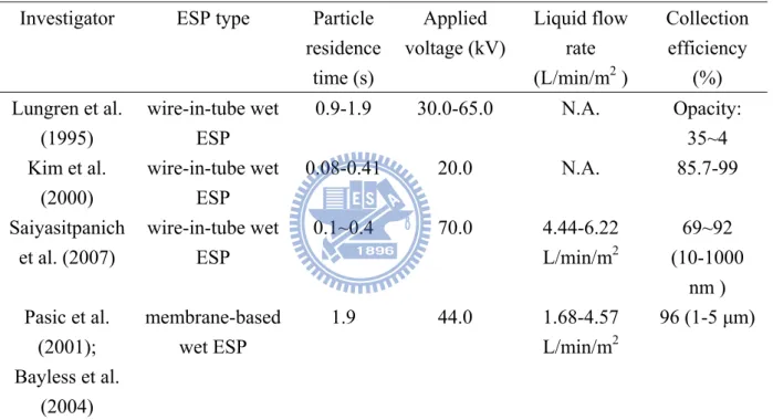
Table 2.1 Literature reviews in experimental studies of wet ESPs.

Investigator ESP type Particle

residence time (s) Applied voltage (kV) Liquid flow rate (L/min/m2 ) Collection efficiency (%) Lungren et al. (1995) wire-in-tube wet ESP 0.9-1.9 30.0-65.0 N.A. Opacity: 35~4 Kim et al. (2000) wire-in-tube wet ESP 0.08-0.41 20.0 N.A. 85.7-99 Saiyasitpanich et al. (2007) wire-in-tube wet ESP 0.1~0.4 70.0 4.44-6.22 L/min/m2 69~92 (10-1000 nm ) Pasic et al. (2001); Bayless et al. (2004) membrane-based wet ESP 1.9 44.0 1.68-4.57 L/min/m2 96 (1-5 μm)

(31)

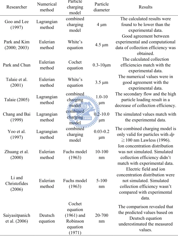
Table 2.2 Literature reviews in numerical studies of particle collection efficiencies in wire-in-plate ESPs. Researcher Numerical method Particle charging model Particle diameter Results

Goo and Lee (1997) Lagrangian method combined charging model 4 μm

The calculated results were found to be lower than the

experimental data. Park and Kim

(2000; 2003)

Eulerian method

White’s

equation 4.5 μm

Good agreement between experimental and computational data of collection efficiency was

obtained. Park and Chun Eulerian

method

Cochet

equation 0.3-10μm

The calculated collection efficiencies match with the

experimental data. Talaie et al. (2001) Eulerian method White’s equation 3.5 μm

The numerical values were in good agreement with the

experimental data. Talaie (2005) Lagrangian method combined charging model 1.0-10 μm

The secondary flow and the high particle loading result in a decrease of collection efficiency. Chang and Bai

(1999) Lagrangian method combined charging model 0.2-10.0 μm

The simulated values match with the experimental data. Yoo et al. (1997) Lagrangian method combined charging model 0.03-0.2 μm

The combined charging model is only valid for particles with dp

≧100 nm Lawless (1996). Zhuang et al. (2000) Eulerian method Fuchs model (1963) 10-100 nm

Ion concentration distribution was not simulated. Simulated collection efficiency didn’t match with experimental data. Li and Christofides (2006) Eulerian method Fuchs model (1963) 5-100 nm

Electric field and ion concentration distribution were

not simulated. Simulated collection efficiency wasn’t compared with experimental

data. Saiyasitpanich et al. (2006) Deutsch equation Cochet equation (1961) and Robinson equation (1971) 20-700 nm

The comparison revealed that the predicted values based on

Deutsch equation underestimated the measured

(32)

CHAPTER 3 METHODS

3.1 Experimental method

3.1.1 The present parallel-plate wet ESP

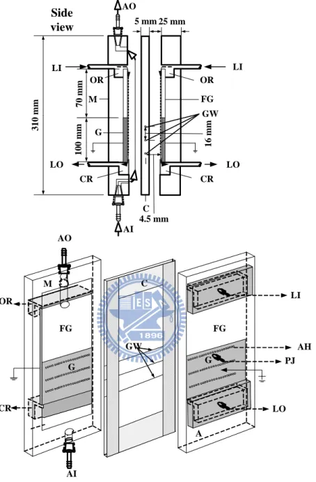
The collection electrodes of the present parallel plate wet ESP were designed based the parallel-plate wet denuder in Tsai et al. (2008). As shown in Figure 3.1, the wet ESP consists of two plexiglass plates (M) on which a copper plate (G) (100 mm in length, 75 mm in width and 3.0 mm in thickness) was attached to the inner surface. A copper plate was used as collection electrode because of its high conductivity and ease with sandblasting. In order to make scrubbing water film flow uniformly on the collection electrodes (G) at low flow rates, a frosted glass plate (FG, 70 mm in length, 75 mm in width and 3.0 mm in thickness) coated with TiO2 nanopowder (Degussa AEROXITE TiO2 P25, Anatase, 20 nm) is attached to the

inner surface (M) above the copper plate. Between the collection electrodes, a center piece (C) is sandwiched to form a 9 mm gap between the electrodes. On the center piece, three gold discharge wires (GW) (99% purity, 100 μm in diameter, Surepure Chemetals Inc.) spaced at 16 mm in the flow direction are fixed. These gold wires were used as discharge wires due to their long lifetime of more than 6 months (Asbach 2004). Two overflowing (OR) and collection reservoirs (CR) for continuous scrubbing water flow are installed at the top and bottom of the ESP, respectively. A pulse jet valve (Bag Filter Enterprise Co. Ltd., Taiwan) was used to generate pulse jet passing through 3 rows of small holes (diameter: 1.0 mm, 24 holes on each row) on the collection plates. The discharge wires were cleaned every 5 minutes with an instantaneous pressure of 2.95 atm (3.05 kg/cm2) and the instantaneous air flow rate passing through all 24 holes per wire was calculated to be 11 L/s. Pulse duration was about 0.5 sec. During pulse jet cleaning, the scrubbing water flow was stopped for two minutes to prevent sparking over due to the water mist generated by the pulse jet.

(33)

LI LI LO LO AI AO M FG OR OR CR CR G LO LI A C GW M AO AI OR CR G PJ AH G FG FG G GW C Side view 31 0 m m 25 mm 100 mm 70 m m 5 mm 4.5 mm 16 mm

Figure 3.1 Schematic diagram of the parallel-plate wet ESP. Plexiglass plates (M), enter piece (C), frosted glass plate (FG), sand-blasted copper plate (G), overflowing reservoir (OR), collecting reservoir (CR), golden wire (GW), liquid inlet (LI), liquid outlet (LO), aerosol inlet (AI), aerosol outlet (AO), pulse jet valve (PJ), air hole (AH).

(34)

In order to increase the hydrophilicity of the collection plates, which will enhance the uniformity of the water film and reduce the scrubbing water flow rate, the copper plate surfaces were first sand blasted to an average depth of 61.0 μm and then coated with TiO2

nanopowder (Degussa P25) based on the method described in Tsai et al. (2008). The surfaces were first sonicated with DI water (18.2 MΩ-cm) and then dried by purging with compressed air. 0.5 g of TiO2 nanopowder was well dispersed in 50 ml DI water by ultrasonication and

then applied onto the sand blasted surfaces. 30 min later, the excess solution was removed, and the plates were calcinated at 300 °C for 90 min to facilitate thermal bonding of the TiO2

nanopowder onto the copper plate surfaces.

Tap water was used as the scrubbing liquid for the collection electrodes. Two peristaltic pumps (Model MP-1000, Eyela Co., Japan) were used to continuously pump water into and out of the overflow and collection reservoirs. The appropriate scrubbing water flow rate, important to water film thickness and uniformity (Tsai et al. 2008), was determined in this study. The goal was to minimize the flow rate in order to decrease the water waste and film thickness (which decreases the electric field due to water’s resistivity), while also ensuring the film is uniform.

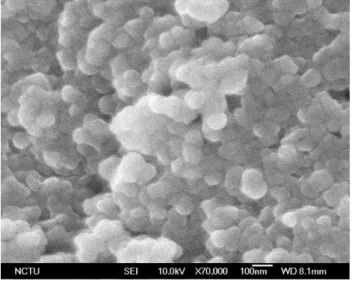
To determine the hydrophilicity of the coated surfaces, the morphology of the TiO2

nanopowder coated on the frosted copper plate was first determined by SEM, and then the water contact angle was measured by using a Contact Angle System (FTA125, First Ten Angstroms, VA). As shown in Figure 3.2, there is a porous surface in our case which is not the same as the water-repellent leaves with epicuticular wax crystals in combination with papillose epidermal observed by Barthlott and Neinhuis (1997). When the water contact angle was measured, we found the frosted surface coated with TiO2 nanopowder sucked in the water

droplet forcing the droplet to spread out quickly. The contact angle was measured to be only 6.0±4.2°, which is very small compared to 104.03±1.73° and 117.17±2.83° for the smooth copper plates and uncoated sand-blasted copper plates, respectively, as shown in Figure 3.3. It

(35)

is certain that hydrophilicity can be achieved by this porous morphology to enhance the uniformity of the scrubbing water film.

Particle collection efficiency experiments were conducted at different aerosol flow rates and applied voltages under initially clean conditions to determine the optimum operation conditions. TiO2 nanopowder was then used to create heavy loading conditions for comparing

(36)

(a)

(b)

Figure 3.2 SEM image of micromorphological characteristic of the frosted copper plate coated with TiO2 nanopowder. (a) X 70,000, (b) X 100,000.

(37)

(a)

(b)

(c)

Figure 3.3 Water contact angle on three copper plate surfaces. (a) smooth surface, (b) sand-blasted surface, and (c) sand-blasted surface coated with TiO2 nanopowder.

(38)

3.1.2 Particle collection efficiency experiment and loading test

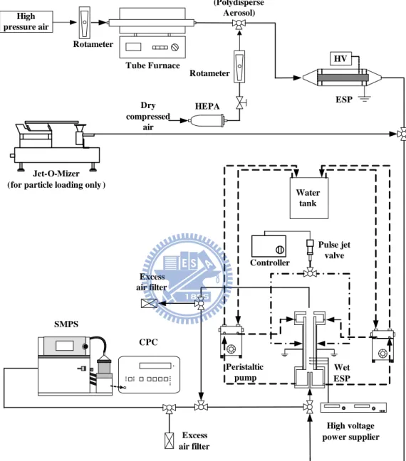
The particle collection efficiency experiments under initially clean conditions were conducted at aerosol flow rates of 5 and 10 L/min (corresponding to residence times of 0.39 and 0.19 seconds, respectively, over the total precipitation length of 48 mm, which is assumed to be three times the wire spacing) with applied voltages ranging from 3.8 to 4.3 kV. The experiment under each operation condition was tested for 6 to 8 hours. The experimental setup is shown in Figure 3.4. Polydisperse liquid corn oil particles (density of 0.9 g/cm3) and silver particles (density of 10.49 g/cm3) were generated by the evaporation-condensation technique (Scheibel et al. 1982) at an oven temperature of 260 and 1050 °C, respectively. Two rotameters were used to control carrier gas and cooling air flow rates to obtain the desired particle diameter and concentration. Before being introduced into the present wet ESP, all charged particles were removed using a wire-in-tube ESP allowing only zero-charged particles to enter the wet ESP. To generate an electric field and corona ions, high positive voltage was supplied to the corona wires using a high voltage D.C. power supplier (Model SL150, Spellman High Voltage Electronics Corporation, NY, USA). The voltage and corresponding corona current were read directly from the power supplier. A scanning mobility particle sizer (SMPS, model 3081, TSI Inc.) coupled with a condensation particle counter (CPC, model 3022, TSI Inc.) was used to measure the size distribution of the polydisperse particles. The characteristics and number size distribution of the test aerosols are shown in Table 3.1, respectively. The particle collection efficiency of the wet ESP, ηtotal(dp), was

calculated by the following equation:

% 100 ) ( ) ( ) ( )(%) (    p in p out p in p total d C d C d C d  (3.1)

where Cin(dp)is the particle inlet concentration (cm-3) and Cout(dp) is the outlet concentration

(39)

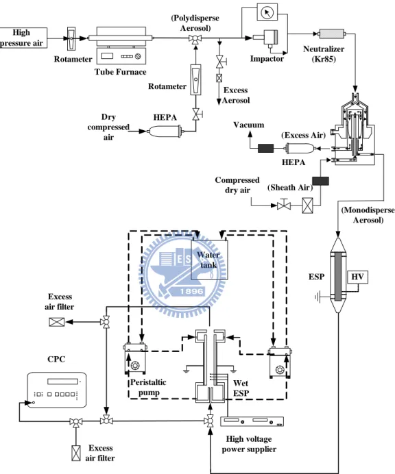
The particle collection efficiency experiment for monodisperse NaCl particle (particle density=2200 kg/m3) was also conducted in this study. The experimental setup is shown in Figure 3.5. Test particles were generated by the evaporation-condensation technique in an oven temperature at temperature of 650 to 700 ℃. The generated particles were then passed through a nano-DMA (differential mobility analyzer, TSI Model 3085) to obtain monodisperse particles with dp of 10 and 50 nm. The experiment was conducted at an aerosol

flow rate of 5 L/min and at an applied voltage of +3.6~+4.3 kV. A condensation particle counter (CPC, model 3022, TSI Inc.) was used to measure particle number concentration. For 10 and 50 nm particles, the inlet concentration of the ESP was measured to be 1.2×109 (m-3) and 6.6×109 (m-3), respectively.

To study particle loading effect on the collection efficiency and possible particle reentrainment after particle loading, Degussa P25 TiO2 nanopowder (resistivity of 0.75×106

Ω·cm) (Salah et al. 2004) was dispersed by a Jet-O-Mizer (Model 000, Fluid Energy Processing and Equipment Co., Hatfield, UK) at an aerosol flow rate of 5.67~56.62 L/min corresponding to a mass loading rate of 0.1-100 g/hr as shown in Figure 3.4. The particles that penetrated through the ESP (Wout, g) and the particles in the excess flow (Wex, g) were

measured by weighing the filters at the outlet of the wet ESP and the excess flow. After loading for two hours, the quantity of particles in the ESP per plate, Wloaded (g), was then

calculated to be 1.2±0.06 g/plate by the following equation:

2 excess outlet total loaded W W W W    (3.2)

where Wtotal (g) is the total particle dispersed by the Jet-O-Mizer. In order to examine the

collection efficiency of the present wet ESP for nanosized particles after 0.5~2 hr of heavy TiO2 particle loading, corn oil particles were used instead of TiO2 nanopowders (P25) because

(40)

very few particles below 100 nm were generated by standard dispersive technique as found in Tsai et al. (2009). A small-scale powder disperser (SSPD, model 3433, TSI Inc.) was also used to disperse the TiO2 nanopowder for conducting the loading test (size distribution is

shown in Table 3.1). However, the mass concentration was too low to generate the desired heavy loading condition. Therefore, corn oil particles generated from the evaporation-condensation technique were used to test the collection efficiency after heavy TiO2 particle loading.

To examine possible redispersion of particles into gas stream after heavy TiO2

nanoparticle loading in the dry ESP, a particle reentrainment test was conducted. After two hours of loading, clean air at a flow rate of 5 L/min was introduced into the dry ESP when the applied voltage was 4.3 kV. The scanning mobility particle sizer (SMPS, model 3081, TSI Inc.) was used to measure the reentrained particle size distributions at 135 second sampling interval.

(41)

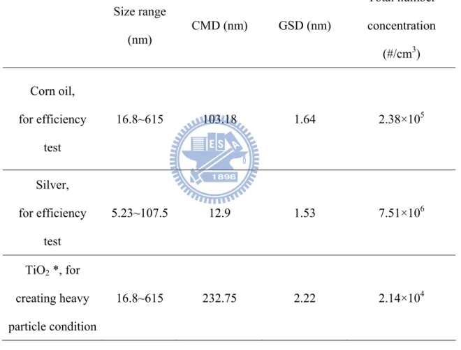
Table 3.1 Characteristics of the test particles Size range (nm) CMD (nm) GSD (nm) Total number concentration (#/cm3) Corn oil, for efficiency test 16.8~615 103.18 1.64 2.38×105 Silver, for efficiency test 5.23~107.5 12.9 1.53 7.51×106 TiO2 *, for creating heavy particle condition 16.8~615 232.75 2.22 2.14×104

(42)

Controller HEPA (Polydisperse Aerosol) ESP HV Excess air filter High voltage power supplier Peristaltic pump Dry compressed air Rotameter Tube Furnace High pressure air Rotameter Jet-O-Mizer (for particle loading only )

SMPS CPC Water tank Wet ESP Pulse jet valve Excess air filter

(43)

Tube Furnace High pressure air Rotameter Compressed dry air Vacuum HEPA (Excess Air) (Sheath Air) (Monodisperse Aerosol) HEPA (Polydisperse Aerosol) Dry compressed air Rotameter _Excess Aerosol Neutralizer (Kr85) Impactor ESP HV Excess air filter High voltage power supplier Peristaltic pump CPC Water tank Wet ESP Excess air filter

(44)

3.2 Numerical method

3.2.1 Flow field

The calculation domains for the dry ESP of Huang and Chen (2002) and the wet ESP (Lin et al. 2010) are shown as the hatched areas in Figures 3.6 (a) and (b), respectively. The dimensions of the present wet ESP were described in the previous experimental method section. The wire-in-plate dry ESP in Huang and Chen (2002) was 300 mm in length, 120 mm in width, and 76 mm in height. Three discharge wires had the diameter of 0.3 mm. The wire to wire spacing and wire to plate spacing was 42 and 60 mm, respectively.

A total of 19,368 (269 in x-direction, 72 in y-direction) non-uniform rectangular girds were used in each of the calculation domains. The average grid size was about 62.5 and 372 μm in x and y direction. The smallest size of 2.35 and 1.94 μm was assigned near the wall of the collection plate of the ESP in Huang and Chen (2002) and the present wet ESP, respectively. It was found that increasing the number of girds from 269×72 to 269×92 only resulted in a slight decreasing of particle diffusion loss from 38.5 to 37.6 % for 10 nm particles in the present wet ESP. Thus, a fixed number of grid of 269×72 was used in the present simulation. The total number of iterations to reach convergence was about 10000 for solving the flow field.

The laminar flow field model was used in both cases because the flow Reynolds numbers based on the hydrodynamic diameter were 130.5 and 1124.4 in the wet ESP (Lin et al. 2010) and the dry ESP (Huang and Chen 2002), respectively, which were all smaller than 2000 (Hinds, 1999). The governing equations for the 2-D Navier-Stokes equations are

                           2 2 2 2 y u x u x P y u v x u u _air air   (3.3)

(45)

                           2 2 2 2 y v x v y P y v v x v u _air air   (3.4)

and the continuity equation is

0       y v x u (3.5)

where u and v (m/s) is the air velocity in x and y direction, respectively, and P is the pressure (Pa). The Navier-Stokes and continuity equations were discretized by means of the finite volume method and solved by the SIMPLER algorithm (Semi-Implicit Method for Pressure-Linked Equations) (Patankar, 1980).

3.2.2 Electric field and ion concentration distribution

The governing equation, Poisson’s equation, for the electric potential distribution in the ESP was written as follows

0 2 2 2 2  _i y V x V __      (3.6)

where V is the potential (Volt), ρi is the space charge density (C/m3).

The space charge density ρi in equation (3.6) were calculated by convection-diffusion

equation for ion concentration distribution as follows

_                   2 2 2 2 ) ( ) ( y x D y Z E v x Z E u _i _i i i i y i i i x i       (3.7)

(46)

where Di is the ion diffusion coefficient (m2/s), Zi is the ion mobility (m2/s-V)), Ex and Ey is

the local electric field at x and y direction (Volt/m), respectively, which can be calculated as

x E x V     (3.8) y E y V     (3.9)

Equations (3.6) and (3.7) were discretized by using the finite volume method and solved by the same computer code used in the flow field simulation. About 100000 iterations were needed to reach convergence. In equation (3.6), the sink term of the ion quenching of particles was neglected because the predicted ion concentration was much higher than the particle number concentration in this study. For example, when the applied voltage was +3.7 kV and -15.5, the average ion number concentration was calculated to be 2.26×1014 and 1.86×1014 (m-3) in the dry and wet ESP, respectively, which was four orders of magnitude higher than the particle concentration. Similarly, in equation (3.7), the source term of the corona current generated by charged particles was neglected, either. To solve Equations (3.6) and (3.7), the ion density at the discharge wire surface must be calculated first as (McDonald et al. 1977)

3 2 1 0 , 10 ) ( 9 30 2 _          c c i p x i r f r Z J s     (3.10)

where sx is the half wire to wire spacing (m), rc is the wire radius (m), f is the wire roughness

factor, δ is the relative density of air, and Jp is theaverage current density at the plate (A/m2).

(47)



2



₀



 

₁



3 0 ₁₉₂ 16s V V s E Z J _c _y y i p        (3.11)







2 1 2 1 . 0 12 9V V_cs_yE  s_yE  



(3.12) c eff x c r r s V E ln 2 1   (3.13) c eff c c c r r E r V  ln (3.14)  y eff s r  4 for 2.0 x y s s (3.15)            c c _TP_r P T TP P T f E 0 0 0 0 6 ₀_.₀₃ 10 3 (3.16)

where V0 is the applied voltage (V), Vc is the corona onset voltage (V), reff is the equivalent

cylinder radius (m), Ec is the corona initiating electric field (V/m), T0=293 (K), P0=1 (atm).

After obtaining Jp, the total current I (A) per discharge wire is calculated as (McDonald et al.

1977)

I J_p4s_xl (3.17)

(48)

Symmetric line Collection plate Calculation domain Aerosol inlet 0.06 0.042 0.3 3 Discharge wires OD=3×10-4 (a) Symmetric line Collection plate Calculation domain Aerosol inlet 0.0045 0.008 0.1 3 Discharge wires OD=10-4 (b)

Figure 3.6 Calculation domain (a) the single-stage wire-in-plate dry ESP (Huang and Cheng 2002), (b) the single-stage wire-in-plate wet ESP (Lin et al. 2010). (unit: m)

(49)

3.2.3 Particle collection efficiency based on Eulerian method

The governing equation of the concentration of particles carrying q elementary charges, Np,q, is p c q p q p B q p p y q p q p p x q p _S _S y N x N D y N Z E vN x N Z E uN                        2 , 2 2 , 2 , , , , ) ( ) ( (3.18)

where ZP is the particle electrical mobility (m2/s-V), which is defined by Zp qeCc/3airdp,

DB is the Brownian diffusion coefficient for particles (m2/s), Sc is the source term, which

represents the generation of particles with q-1 charges. In the turbulent flow case, DB is

replaced by Deddy (m2/s) calculated by equations (2.5)-(2.11) as described in section 2.2. In

equation (3.18), the source term Sc and sink term Sp are given by (Adachi et al. 1985; Aliat et

al. 2009) i q p q c N N S  _₁ _, _₁ (3.19) i q p q p N N

S  _, for particles with q elementary charges (3.20)

where αqis the combination coefficient of ions for particles carrying q elementary charges

(m3/s), which is given by (Fuchs, 1963)

 







                      _  r a b i r i b r b r r i q dx T k x a a D c T k T k c           / 0 2 2 / exp 4 exp 1 exp (3.21)

一個控制細微粒及奈米微粒排放的電極線-平板型濕式靜電集塵器

國

立

交

通

大

學

環境工程研究所

博

士

論

文

一個控制細微粒及奈米微粒排放的

電極線-平板型濕式靜電集塵器

A Wire-in-Plate Wet Electrostatic Precipitator for Controlling

Fine and Nanosized Particle Emission

研 究 生：林冠宇

指導教授：蔡春進 教授

一個控制細微粒及奈米微粒排放的

電極線-平板型濕式靜電集塵器

A Wire-in-Plate Wet Electrostatic Precipitator for Controlling

Fine and Nanosized Particle Emission

研 究 生：林冠宇

Student：Guan-Yu Lin

指導教授：蔡春進

Advisor：Chuen-Jinn Tsai

國 立 交 通 大 學

環境工程研究所

博 士 論 文

中華民國九十九年八月

一個控制細微粒及奈米微粒排放的

電極線-平板型濕式靜電集塵器

學生：林冠宇

指導教授：蔡春進

國立交通大學環境工程研究所

摘要

A Wire-in-Plate Wet Electrostatic Precipitator for Controlling

Fine and Nanosized Particle Emission

Student: Guan-Yu Lin

Adviser:Dr. Chuen-Jinn Tsai

Institute of Environmental Engineering

National Chiao Tung University

ABSTRACT

TABLE OF CONTENTS

LIST OF TABLES

LIST OF FIGURES

LIST OF SYMBOLS

CHAPTER 1

INTRODUCTION

CHAPTER 2

LITERATURE REVIEW

CHAPTER 3

METHODS







 











 

 







研究生：林冠宇

指導教授：蔡春進教授

研究生：林冠宇

國立交通大學

博士論文

學生：林冠宇　　　