國立交通大學
經營管理研究所
博
士 論 文
No. 130
國際能源價格衝擊對台灣總體經濟活動之影響
Effects of International Energy Price Shocks on
Macroeconomic Activities in Taiwan
研 究 生:葉芳瑜
指導教授:胡均立 教授
國
立
交
通
大
學
經營管理研究所
博
士 論 文
No. 130
國際能源價格衝擊對台灣總體經濟活動之影響
Effects of International Energy Price Shocks on
Macroeconomic Activities in Taiwan
研 究 生:葉芳瑜
研究指導委員會:胡均立 教授
丁 承 教授
林介鵬 教授
指導教授:胡均立 教授
中
華 民 國 九十九 年 六 月
國際能源價格衝擊對台灣總體經濟活動之影響
Effects of International Energy Price Shocks on
Macroeconomic Activities in Taiwan
研 究 生: 葉芳瑜 Student: Fang-Yu Yeh
指導教授: 胡均立 Advisor: Dr. Jin-Li Hu
國 立 交 通 大 學
經 營 管 理 研 究 所
博 士 論 文
A Dissertation Proposal
Submitted to Institute of Business and Management College of Management
National Chiao Tung University in Partial Fulfillment of the Requirements
for the Degree of Doctor of Philosophy in
Business and Management May 2010
Taipei, Taiwan, Republic of China
國際能源價格衝擊對台灣總體經濟活動之影響
Effects of International Energy Price Shocks on
Macroeconomic Activities in Taiwan
研究生:葉芳瑜
指導教授
:胡均立
教授
國立交通大學經營管理研究所博士班
中文摘要
台灣為一能源有限且能源進口依存度高達99.32 %的海島型經濟體。隨著國 際能源價格不斷攀高,國際能源價格的變動對台灣總體經濟活動之影響將值得深 入研究。本論文利用線性與非對稱的架構去評估國際能源價格(原油、煤炭、天 然氣)與台灣總體經濟變數(工業生產指數、股價、利率、失業率、進口值與出口 值等)之間的關係。利用 Tsay (1998) 所提出的多變量門檻模型結合非對稱動態調 整過程加以分析,以能源價格變動當作一個門檻變數區分為能源價格上漲與下跌 狀態,檢視在不同狀態下國際能源價格衝擊對台灣總體經濟活動的影響,進一步 利用衝擊反應分析與變異數分解去評估能源價格波動對台灣總體經濟之衝擊。研 究結果顯示:(1)油價的最適門檻值 2.48%,其次為天然氣價格門檻值 0.87%,最 小為煤價門檻值0.22%;(2)當油價大於門檻值時,油價對於工業生產值上的解釋 能力更甚於利率;(3)當天然氣價格小於門檻值時,天然氣價格分別在股價與失 業率上面都具有較大的解釋能力;(4)煤價衝擊與天然氣價格衝擊均對於台灣總 體經濟活動而言具有延遲的負面影響。 關鍵詞:能源價格衝擊、總體經濟活動、多變量門檻誤差修正模型、衝擊反應分 析、變異數分解Effects of International Energy Price Shocks on
Macroeconomic Activities in Taiwan
Student: Fang-Yu Yeh Advisor: Dr. Jin-Li Hu
Institute of Business and Management
National Chiao Tung University
Abstract
Taiwan is an island with limited domestic energy resources and its imported energy ratio is over 99.32%. As international energy prices keep rising, the impacts of this on Taiwan’s economic activities have been an important issue of research. This paper applies a linear and asymmetric model to estimate the effects of international energy price shocks (including oil, coal, and natural gas prices) on Taiwan’s macroeconomic activity (such as industrial production, stock price, interest rate, unemployment rate, imports and exports). We apply a multivariate threshold error correction model by Tsay (1998) to analyze the empirical data. By separating energy price changes into the decrease and increase, the energy price change as a threshold variable can analyze different impacts of energy price changes and their shock on industrial production. The variance decomposition and the impulse response functions are also employed to analyze the short-run dynamics of the variables. The preliminary findings are: (1) The optimal threshold levels are that the highest level is oil price at 2.48%, the next highest is natural gas price at 0.87%, and the lowest level is coal price at 0.22%. (2) If the change is above the threshold
levels, then a change in oil price explains industrial production better than the interest rate. (3) If the change is below the threshold levels, then it appears that the change in natural gas price better explains stock prices and the unemployment rate than the interest rate. (4) Both oil price shock and natural gas shock have a delayed negative impact on macroeconomic activities.
Keywords: Energy Price Shocks; Macroeconomic Activity; Multivariate Threshold Error Correction (MVTEC) Model; Impulse Response Analysis; Variance Decomposition
Acknowledgements
First, I would like to express my deep and sincere gratitude to my thesis advisor, Prof. Jin-Li Hu, for his direction, assistance, and guidance for almost six years. He is the most erudite and kindest person I have ever met. His warm encouragement and help made me feel confident to fulfill my desire and to overcome every difficulty I encountered.
Next, I would express special thanks to Prof. Cherng G. Ding and Prof. Chieh-Peng Lin for providing detailed instructions and suggestions for this dissertation. I would also like to express my gratitude to Prof. Hsien-Chang Kuo, Prof. Wun-Hua Chen, Prof. Shih-Mo Lin, and Prof. Yung-Ho Chiu for their valuable comments which have enriched this dissertation for a great extent. For the administrative assistance, I would like to thank the Ms. Hsiao, Ms. Wang, Ms. Liao, Ms. Hsieh in the Ph.D. program for their patience handling the process throughout my graduate studies.
In addition, I would heartily thankful to my betrothed and best friend, Dr. Cheng-Hsun Lin, for his sincere supervision, fruitful guidance and valuable advice throughout my academic work. At the last stage of my academic work, he always been there every time, taken my weakness and made me strong. His considerate and caring are not sufficient to express my gratitude with only a few words. For the next journey in my life, I expect that I will be your shelter thru the raging storm and you will be the wings that guide my broken flight. As you said that time will take away our youth but our love and promise will never be changed.
Finally, I would like to share my pleasure of graduation to my lovely family, Chen-Nan Yeh, Pi-Ju Shih, Mei-Chun Yeh, Shu-Wei, Yeh. Words are inadequate to express my thanks to you. Your wisdom, patience, and selfless concern for me are my greatest engine of growth. Special thanks should be given to others who accompany me but not being mentioned for their friendship and kindness during my years in NCTU. This thesis is dedicated to my parents and I’ll love you forever.
Table of Contents
Chinese Abstract ...i
English Abstract ...ii
Acknowledgements ...iv
Table of Contents ...vi
List of Tables...vii
List of Figures...viii
Chapter 1 Introduction... 1
1.1 Research Background ... 1
1.2 Research Motivation and Purpose ... 5
1.3 Organization of the Dissertation ... 7
Chapter 2 Literature Review ... 9
2.1 Impact of Oil Price on GDP... 9
2.2 Impact of Oil Price on Other Macroeconomic Variables... 11
2.3 Price Effects of Natural Gas and Coal ... 15
Chapter 3 Methodology ... 21
3.1 Unit Root Tests... 22
3.1.1 Augmented Dickey Fuller (ADF) Test ... 22
3.1.2 Kwiatkowski, Phillips, Schmidt, and Shin (KPSS) Test ... 24
3.2 Cointegration Analysis... 26
3.3 Multivariate Threshold Error Correction (MVTEC) Model ... 28
3.4 Impulse Response Analysis... 31
3.5 Variance Decomposition ... 36
Chapter 4 Empirical Results... 38
4.1 Data Description ... 38
4.2 One-regime VAR analysis... 39
4.2.1 Results of Tests for Unit Roots and Cointegration ... 39
4.2.2 Results of the Variance Decomposition... 42
4.2.3 Results of the Impulse Response Analysis ... 45
4.3 Two-regime VAR analysis ... 48
4.3.1 Estimating the Threshold Levels and the Delay of Threshold Variables. 48 4.3.2 Results of the Variance Decomposition in the MVTEC Model ... 49
4.3.3 Results of the Impulse Response Analysis in the MVTEC Model... 54
4.3.4 Results of the Parameter Stability Tests ... 59
Chapter 5 Preliminary Conclusions and Policy Implications... 63
References ... 67
List of Tables
Table 2.1 An Overview of Previous Studies of the Impacts of Energy Price Shocks on
Industrial Production and Macroeconomics Activities, 1999-2009...17
Table 4.1 Definitions of Variables...39
Table 4.2 Results of Unit Root Tests...40
Table 4.3 Results of the Johansen Cointegration Tests ...42
Table 4.4 Variance Decompositions of Forecast Error Variance in One-regime VAR Model (12 Periods Forward) ...43
Table 4.5 Results of Threshold Effect Tests...48
Table 4.6 Variance Decomposition Results Using Oil Price Changes as Threshold Variable (12 Periods Forward)...50
Table 4.7 Variance Decomposition Results Using Coal Price Changes as Threshold Variable (12 Periods Forward)...51
Table 4.8 Variance Decomposition Results Using Natural Gas Price Change as Threshold Variable (12 Periods Forward) ...53
List of Figures
Figure 1.1 World Marketed Energy Price, 1983-2009... 1 Figure 1.2 World Marketed Energy Use by Fuel Type, 1980-2030... 3 Figure 1.3 The Co-movement Between Domestic Energy Price Index and WTI Oil
Price Index, 1971-2008... 4 Figure 1.4 Research Flow Chart ... 8 Figure 3.1 Methodology Flow Chart ...21 Figure 4.1 Impulse Responses from One Standard Deviation Shock of Energy Price
Change in the Linear VAR Model (12 Periods Forward). ...46 Figure 4.2 Impulse Responses from One Standard Deviation Shock of Energy Price
Change in the Regime One VAR Model (12 Periods Forward). ...55 Figure 4.3 Impulse Responses from One Standard Deviation Shock of Energy Price
Change in the Regime Two VAR Model (12 Periods Forward) ...56 Figure 4.4 Plots of the CUSUM and CUSUM of Square Test in Regime Ono. ...61 Figure 4.5 Plots of the CUSUM and CUSUM of Square Test in Regime Two. ...62
Chapter 1 Introduction
1.1 Research Background
Energy price shocks are generally acknowledged to have important effects on both the economic activity and macroeconomic policy of industrial countries. Huge and sudden rises in energy prices increase inflation and reduce real money balances with negative effects on consumption and output. Among the most acute supply shocks hitting the world economies since World War II are sharp increases in the price of oil and other energy products. Figure 1.1 shows the annual average energy price (oil price, natural gas price, and coal price) from 1983 to 2009.
Figure 1.1 World Marketed Energy Price, 1983-2009
0 50 100 150 200 250 1983 1984 1984 1985 1986 1987 1988 1989 1990 1991 1992 1993 1994 1995 1995 1996 1997 1998 1999 2000 2001 2002 2003 2004 2005 2006 2006 2007 2008 US D ollars per Barrel \ M etric T on
Oil price (WTI) Natural gas price (Russia) Coal price (Australia) invaded Kuwait Asian financial crisis OPEC production restraint Iraq War Hurricane shut down production Yukos Bankruptcy and Strikes in Nigeria
Coal price Oil price Gas price increase Saudi production Iraq
Since the 1970s, oil price in the world market has experienced fluctuations including sharp rises during the first and second oil crises. During the periods of 1973-1974 and 1978-1979, when the Organization of Petroleum Exporting Countries (OECD) first imposed an oil embargo and the Iranian revolution disrupted oil supplies, the prices of a barrel of oil increased from $3.4 to $30. In 1990, prices rapidly rose from $16 to $26 after the Gulf War. Finally, due to a decline from the Asian financial crisis in 1999, prices fell from $20.28 to $11.13. Since 2000, oil prices have continued an upward trend with repeated fluctuations. In particular, oil price volatility in the crude oil market has risen during 2004 to 2008. By March 13, 2008, the oil price had spiked to a historical high of $110.21 per barrel (West Texas Intermediate (WTI) spot). Recently, the WTI oil future prices averaged $76 per barrel in October 2009 on the New York Mercantile Exchange (NYMEX). This is an increase of just over 8 percent for this month. EIA (2009) estimates that the January 2010 WTI futures contract consistent with this volatility was $61 per barrel at the lower limit and $104 per barrel at the upper limit for the 95 percent confidence interval.
Higher prices of oil driving demand for other energy have made natural gas and coal more competitive (see Figure 1.2). From 1986 to 1999, natural gas prices averaged $1.87 per million cubic feet (mcf), with a standard deviation of $0.24 per year (Kliesen, 2006). Since 2001, natural gas prices began to rise noticeably. Natural gas prices in both real and nominal dollars were at record-high levels by 2005. In 2008, natural gas prices averaged approximately $9 per mcf. Because price-setting is based on production costs and applications for rate increases move slowly through the bureaucratic process, natural gas volatility is quite small. On average, natural gas price variability is 3%-4%.
Natural Gas (average 106.3) Coal (average 123.2) Nuclear (average42.7) Renewables (average 26.9) 0 50 100 150 200 1980 1989 1998 2007 2016 2025 Year Quadrillion Btu
Figure 1.2 World Marketed Energy Use by Fuel Type, 1980-2030
Sources: Energy Information Administration, International Energy Annual 2006
Coal is similarly the primary factor for industrial revolution in the world. In 2006 coal was the world’s fastest-growing used fuel with global consumption rising by 5% per annum. The monthly average coal price reached a record high of $208.55 per mcf in 2008. Coal prices saw severe fluctuations during 2003 to 2009.
At the regional level, oil is of particular importance to many Asian economies as most are net importers of this energy product. Because Taiwan is an island with limited indigenous energy resources and energy imports are over 99.32% in 2008, Taiwan has been identified as one of six Asian economies (including Japan, Philippines, Singapore, South Korea, Taiwan, and Thailand) that are considered to be easily subjected to world oil price fluctuation (Aoyama and Berard, 1998). Figure 1.3 illustrates the co-movement of Taiwan’s domestic energy prices indices (including fuel oil, coal, natural gas, gasoline, and diesel oil) with fluctuations of the WTI oil price index since 1971. We observe that the former variables are linked to the latter’s trend.
0 50 100 150 200 250 300 1971 1975 1979 1983 1987 1991 1995 1999 2003 2007 U S Do ll ars p er B arre l
WTI Gasoline Diesel Oil Fuel Oil Coal Natural Gas
Figure 1.3 The Co-movement Between Domestic Energy Price Index and WTI Oil Price Index, 1971-2008
Domestic energy price-setting is relatively affected by projected world oil prices in the past several years. Jiménez-Rodríguez and Sánchez (2005) report that oil price increases have a direct impact on economy activity for oil-importing countries. Indeed, rising oil prices are interpreted as an indicator of an increase in scarcity and that means oil will be less available on the domestic market. This phenomenon is expected to keep the domestic energy price at high levels over the near term.
World oil shocks not only directly affect domestic energy prices, but also imply the importance of domestic renewable industry development. To expedite domestic energy diversity as well as improve environment quality, a number of Taiwan’s factories have developed a renewable industry since 1998. Through Taiwan’s innovative pattern of learning-by-doing which borrows much production knowledge from its
semiconductor production, the renewable industry such as photovoltaic is currently in the value inflow stage (Hu and Yeh, forthcoming). Compared to other countries, Taiwan ranks as the fourth largest solar cell producing country in the world. The empirical analysis of this dissertation highlights the status of its importance.
In sharp contrast to the volume of studies examining the link between oil price shocks and macroeconomic variables, there is currently not much existing literature on quantitative analyses of coal-price or gas-price shocks. There are also few analyses on the relationship between oil price shocks and financial markets such as the stock market. Market participants want a framework that identifies how energy price changes affect the stock market and labor market.
1.2 Research Motivation and Purpose
As energy prices play a critical role in influencing economic growth and economic activities, this phenomenon excites the research interest of this dissertation to address a linkage analysis of international energy prices and macroeconomic variables in Taiwan with linear and non-linear frameworks. Our research is motivated by the following reasons.
First, most studies (e.g., Burbidge and Harrison, 1984; Gisser and Goodwin, 1986; Mork, 1989; Hooker, 1996; Hamilton, 1996; Bernanke et al., 1997; Hamilton, 2003; Hamilton and Herrera, 2004) show that oil price shocks have a significantly negative impact on industrial production. However, little is known about the relationship between other energy prices and economy activities. For this reason, researchers may refocus their attention on the issue of natural gas price and coal price and their impact on economic activities.
Sadorsky, 1999; Papapetrou, 2001; Hu and Lin, 2008) already consider the asymmetrical relation in terms of the impact of an oil price change or its volatility on industrial production and stock returns. However, these studies arbitrarily use zero as a cutoff point and distinguish oil price changes into up (increase) and down (decrease). This shows that the traditional approaches using predetermined value(s) as a demarcation point are rather unreasonable. They neglect the asymmetrical relation to accurately gauge varying degrees of impacts of energy price change (or volatility) on macroeconomy. To solve the neglected phenomenon, we implement rigorous econometric methods to refine the true relation.
Third, early studies about the macroeconomic consequences of energy price shocks focus on developed economies. Recent studies examine other research samples such as European countries (e.g., Mork et al, 1994; Papapetrou, 2001; Cunado and Pérez de Gracia, 2003; Jiménez-Rodríguez, 2008; Bjørnland, 2009) and Asian countries (e.g., Chang and Wong, 2003; Cunado and Pérez de Gracia, 2005; Huang et al., 2005). However, few studies investigate the relationship between energy price and macroeconomy for Taiwan. In contrast to these studies, this dissertation assesses the dynamic effect of energy price shocks on the macroeconomy in Taiwan.
Based on the aforementioned argument, the purposes of this dissertation contain two parts: The first purpose is to examine the effects of energy price shocks (including crude oil, natural gas and coal) on Taiwan’s industrial production from a linear perspective. Energy prices do not affect industrial production in isolation, but through the perceived effect on the macroeconomy. Therefore, we further analyze the dynamic relationship between energy price shocks and major macroeconomic variables (including stock price, interest rate, unemployment rate, exports and imports) by applying a vector error correction (VECM) model. Next, the variance decomposition (VDC) and the impulse response functions (IRF) are employed to capture the effects of
energy price shocks on the macroeconomy. The results find how each variable responds to shocks by other variables of the system and explore the response of a variable to a shock immediately or with various lags.
The second purpose focuses on the impacts of an energy price change and the shock on the macroeconomy from an asymmetric perspective. According to Sadorsky (1999), the energy price adjustment may not immediately impact macroeconomic variables. An economic threshold for an energy price impact is the amount of price increase beyond which an economic impact on industrial production and stock prices is palpable. Huang et al. (2005) propose that a change in oil price explains the macroeconomic variables better than the shock caused by the oil price if an oil price change exceeds the threshold levels. Therefore, we apply the multivariate threshold error correction model by Tsay (1998) to analyze the relevant data. By separating energy price changes into decrease (down) and increase (up), the energy price changes as the threshold variable can analyze different impacts of energy price changes on industrial production. In particular, we assess the impact of energy price fluctuations on the Taiwan economy. The impulse response and the variance decomposition analysis now follow.
1.3 Organization of the Dissertation
This dissertation is organized in the following manner as Figure 1.4 shows: Chapter 1 states the motivation and purposes for this study. Chapter 2 reviews the related literature. Chapter 3 gives a brief introduction of research methods. Chapter 4 presents the empirical results of energy price shocks with the linear (one-regime) VECM model and the multivariate threshold error correction (two-regime) model and discusses the result. Chapter 5 concludes with a brief review of the principal findings and a discussion of directions for further study.
Chapter 1 Introduction Research Background
Research Motivation and Purpose Organization of the Dissertation
Chapter 2 Literature Review Impact of oil price on GDP
Impact of oil price on the other macroeconomic variables
Price effects of natural gas and coal
Chapter 3 Methodology Unit Root Tests
Cointegration Analysis
Multivariate Threshold Error Correction Model Impulse Response Analysis
Variance Decomposition
Chapter 4 Empirical Results Asymmetric behavior between energy price and macroeconomic variables
Energy prices shocks and macroeconomic variables changes
Chapter 5 Concluding Remarks
Chapter 2 Literature Review
Since the 1970s many studies have examined the relationship between energy prices and the macroeconomy especially for oil price shocks. However, there is an inconsistent conclusion in the literature with different estimation procedures and data. According to the different energy prices used by researchers, previous studies can be divided into three streams of research: the impact of oil price on GDP, the impact of oil price on other macroeconomic variables, and the natural gas and coal price effect. A survey of the literature on the effects of energy price shocks on macroeconomy now follows.
2.1 Impact of Oil Price on GDP
There are extensive studies that explore the relationship between oil prices and economic activity. In a pioneer work, Hamilton (1983) using Granger causality examines the impact of oil price shocks on the United States economy, indicating that oil price increases partly account for every United States recession. A given oil price increase seems to have had a smaller macroeconomic effect after 1973 than an increase of the same magnitude would have had before 1973. Since then, many researchers extend and reinforce Hamilton’s basic findings using different estimation procedures on new data (e.g., Burbidge and Harrison, 1984; Gisser and Goodwin, 1986; Mork, 1989; Hooker, 1996; Hamilton, 1996; Bernanke et al., 1997; Hamilton, 2003; Hamilton and Herrera, 2004). These studies conclude that there is a significant negative correlation between increases in oil prices and the subsequent recessions in the United States, but that oil price changes have different impacts on economies over time.
Following declines in oil prices during the global energy crisis of the 1980s, the impact from an energy price change and its shock on economic activities disappeared. Some researchers argue that the instability observed in this relationship and the past linear specification have led to the misrepresentation of the measure. Gradually, attention has shifted to asymmetric oil price shocks on economic activities (Mork, 1989; Mork et al., 1994; Lee and Ratti, 1995; Lee et al., 1995; Hamilton 1996; Ferderer, 1996).
By separating oil price changes into negative and positive, Mork (1989) finds that there is an asymmetrical relationship between oil price and real output. When the oil price is increasing, the increase in the cost of production and the decrease in the cost of resource allocation often offset each other. Alternatively, a decrease in oil price will decrease the cost of production. These two forces have a correspondingly significant impact on GDP. Mory (1993) follows Mork’s (1989) measures and presents that positive oil price shocks Granger-cause the macroeconomic variables. Mork et al. (1994) again confirm that an oil price shock induced inflation reduces real balances for seven industrialized countries.
Besides examining the direct effects of oil price changes, some researchers try to use the variable of their volatility to investigate their shock on certain macroeconomic variables. Lee et al. (1995) examine the impact of an oil price change on aggregate economic activities by using a generalized autoregressive conditional heteroskedasticity (GARCH) model. They find that an oil shock in a price stable environment is more likely to have greater effects on GDP growth than those occurring in a price volatile environment. In the same way, Hamilton (1996) points out that the key question is whether the oil price increase is big enough to reverse any decreases observed in the immediate previous quarters. Both Lee et al. (1995) and Hamilton (1996) conclude that there is a negative relationship between increases in oil prices and real output in the
U.S. economy. In the same vein, Hamilton (2003) reports evidence of non-linearity with three earlier pieces of literature (Mork, 1989; Lee et al., 1995; Hamilton, 1996), indicating that oil price increases are much more important than oil price decreases and the formulation of Lee et al. (1995) has the best work.
Jiménez-Rodríguez and Sánchez (2005) use the multivariate VAR model to examine the effects of oil price shocks on real GDP growth in eight OECD countries. They find that oil price increase has a larger impact on GDP growth than oil price declines. A brief summary of the relationship between oil price and GDP is shown in Jones et al. (2004). First, most studies offer that the recessionary movements of GDP are largely attributable to oil price shocks. Second, asymmetric specifications of oil price shocks are found. Third, detailed empirical studies have proposed that a considerable reallocation of labor occurs after oil price shocks.
2.2 Impact of Oil Price on Other Macroeconomic Variables
In addition to exploring the relationship between oil price shocks and GDP, some economists have emphasized the relationship between oil price shocks and other macroeconomic variables. The related issues can be divided into three parts.
The first part is related to the macroeconomic level. Several models (e.g., Rasche and Tatom, 1981; Bruno and Sachs, 1982, Hamilton, 1983) and diverse episodes for oil price shocks (e.g., Davis, 1986; Carruth et al., 1998; Ferderer, 1996) present that an oil shock is one of the important influences on the macroeconomy. The directions for the causal relationship between oil price and macroeconomy can be concluded in four parts. First, oil price changes significantly impact economic activity (e.g., Papapetrou, 2001; Ewing et al., 2006; Jiménez-Rodríguez, 2008; Farzanegan and Markwardt, 2009). Second, there is an asymmetric correlation between oil price and the macroeconomy (e.g., Loungani, 1986; Mork, 1989; Lee et al., 1995; Hamilton, 2003; Cunado and Pérez
de Gracia, 2003; Cunado and Pérez de Gracia, 2005; Jiménez-Rodríguez, 2009). Third, some researchers show effects of oil price shocks at a disaggregate level. For example, Davis and Haltiwanger (2001) analyze the effects of oil shocks on plant level employment. Edelstein and Kilian (2007) examine the effects of oil shocks on U.S. non-residential fixed investment expenditures. Finally, because of the government’s tight monetary policy, economic activity does not originate from an oil price change (e.g., Bernanke et al., 1997; Balke et al., 2002; Hamilton and Herrera, 2004).
Hooker (1996) argues that oil price shocks promote directly to recession remains in some dispute, in part due to the correlation between oil prices and economic activity seems to be much weaker in data obtained since 1985. As can be seen from the aforementioned studies, there are some main channels for oil price shocks to influence economic activities, including consumer price index (e.g., Cunado and Pérez de Gracia, 2005; Jiménez-Rodríguez, 2009; Bjørnland, 2009), stock price (e.g., Park and Ratti, 2008; Apergis and Miller, 2009), exchange rate (e.g., Farzanegan and Markwardt, 2009; Jbir and Zouari-Ghorbel, 2009), and unemployment rate (e.g., Bjørnland, 2009; Jiménez-Rodríguez, 2009). In addition, both Ferderer (1996) and Hooker (1996) suggest interest rates as a channel for oil price shocks to influence economic activity. Impulse response analysis shows that an oil price shock works primarily through the interest rate. There is also a strongly asymmetric response of the short-term interest rate to positive and negative oil price shocks and a modestly asymmetric response from the long-term rate. Park and Ratti (2008) prove that an increase in real oil price is associated with a significant increase in the short-term interest rate in the U.S. and eight out of thirteen European countries with one or two months. For a comprehensive survey of empirical results on the macroeconomic consequences of oil price shocks, see Jones et al. (2004).
The second part is related to stock markets. An increase in oil price causes expected earnings to decline, and this will bring about an immediate decrease in stock prices if the stock market is efficient. If the stock market is not efficient, then there may be lags in adjustment to oil price changes. There are several representative studies about the impact of oil price on stock prices (or stock returns). Those mainly with research data include the United States, United Kingdom, Japan, and Canada. Kaneko and Lee (1995) use a VAR model to estimate the relationship between energy price change and aggregate economic activities (including industrial production growth, inflation, stock prices, and exchange rate) in the U.S. and Japan, and they find that Japanese stock prices are affected by oil price shocks. Jones and Kaul (1996) further investigate the reaction of stock prices to oil price shocks and what may justify these movements. By using a cash-flow/dividend valuation model (i.e., Campbell, 1991), they find that oil prices can predict stock returns and output on their own.
Sadorsky (1999) considers the relationship between oil price shocks and stock returns using a four-variable VAR model. He discovers that oil price movements can explain more of the forecast error variance of stock returns than can interest rates. Beyond that, he shows an asymmetric effect on stock returns from oil price shocks. Increases in the price of oil have a significant effect on reducing stock prices, but not vice versa. There seems to be an asymmetric relation between oil price change (or its volatility) and economic activities (i.e., output, stock returns, and interest rates). This argument is once again re-confirmed by Ciner’s (2001) and Hamilton’s (2003) studies.
Some studies (e.g., Lo and MacKinlay, 1990; Kaul and Seyhum, 1990; Sadorsky, 2003; Park and Ratti, 2008) use the volatility of oil price changes to test its relationship with stock returns. They propose that an increased volatility of oil prices significantly depresses real stock returns. In addition, El-Sharif et al. (2005) provide further background to previous findings on the link between oil prices and measures of stock
market performance. Later studies (e.g., Cong et al., 2008; Park and Ratti, 2008; Apergis and Miller, 2009; Bjørnland, 2009) document the diverse relationship between oil price movements and stock prices. Both Huang et al. (1996) and Cong et al. (2008) find no evidence of the impact of an oil price change on stock returns. However, Park and Ratti (2008) show that the effect of oil price shocks on stock returns is contemporaneous in the U.S. and thirteen European countries. Bjørnland (2009) indicates that following a 10% increase in oil prices, Norway’s stock returns increase by 2.5%. Apergis and Miller (2009) also find that different oil market structural shocks play a significant role in explaining the adjustments in stock returns.
The third part involves the labor market. Several studies address the question of whether there is a correlation between oil price and the labor market. A clear negative relationship between oil prices and employment is reported by Rasche and Tatom (1981), Hamilton (1983), Keane and Prasad (1996), Uri (1996), Raymond and Rich (1997), among others. Keane and Prasad (1996) further indicate that oil price increases reduce employment in the short run, but tend to increase total employment in the long run. The labor market responses may be quicker than previously thought in the shorter run. These results imply a possible substitution between energy and labor in the aggregate production function. Due to the substitute and complimentary abilities among different sectors of the labor market, there is a positive relationship between oil price increases and employment in the long run. Nevertheless, both Loungani (1986) and Kandil and Mirzaie (2003) argue for no evidence that changes in oil prices influence employment growth.
An oil price decrease depresses demand for some sectors, and unemployed labor is not immediately shifted elsewhere (Hamilton, 2003). However, oil price changes impact unemployment when the changes in oil prices persist for a long time as adjustments in employment (Keane and Prasad, 1996). Davis (1986) offers separate
time trends before and after 1974 in his unemployment equations. He finds that the estimated time trend coefficients are small and often statistically insignificant with most of the upward trend in unemployment over these samples. Carruth et al. (1998) present an asymmetrical relationship among unemployment, real interest rates, and oil prices, meaning that oil price increases cause employment growth to decline more than oil price decreases cause employment growth to increase. Davis and Haltiwanger (2001) focus on how oil price movements influence the unemployment rate over time. They use the structural VAR models to measure oil price by a weighted average of real oil prices. The results find an oil price shock can explain 25% of the cyclical variability in employment growth from 1972 to 1988. The long-run relationship result is similar to Keane and Prasad (1996). Lardic and Mignon (2008) summarize six transmission channels of increasing oil prices (i.e., reduction of potential output, increased money demand, inflation including second round effects, negative terms of trade effects for oil importing countries, negative demand side impacts, and structural changes). They also show that a long-lasting oil price increase can thus change the production structures and have an impact on unemployment.
2.3 Price Effects of Natural Gas and Coal
Most studies show the effect of oil price shocks, but rarely consider the effect of natural gas or coal price shocks. Coal and natural gas are the two main alternative sources of energy. There are three effects of changing natural gas price controls: on regional economic activity (e.g., Leone, 1982), on inflation (e.g., Ott and Tatom, 1982), and on the distribution of income between households and suppliers (e.g., Stockfisch, 1982). These results find that the presumed effects of natural gas decontrol (higher price, higher inflation, and falling real incomes) are not expected to be significant. Hickman et al. (1987) examine the correlation between natural gas price and industrial
production. They indicate that a 10% increase in natural gas price affects the same effect on real GDP growth. A permanent $1 increase in natural gas prices will reduce real GDP growth by 0.1 percentage points per year (the Economics and Statistics Administration, 2005).
Jin et al. (2009) examine the effects of energy prices and energy conservation on economic growth for the postwar U.S. economy. They use a five-variable VAR model that consists of real GDP, real capital, real energy prices, labor, and the Divisia energy consumption index. The Divisia index is constructed using expenditures on three major energy resources (i.e., oil, coal, and natural gas). They find that energy prices have significant negative effects on real economic growth and oil price shocks are greater than other resources. These results are consistent with earlier findings in Hamilton (1983) and Burbidge and Harrison (1984). Lutz and Meyer (2009) observe that a stabilizing effect via international trade and domestic structural change on the GDP of oil importing countries with a permanent oil price increase occurs. At least for Germany, it is not negatively influenced by higher oil and natural gas prices, even though a strong structural divergence can be observed.
Researchers have begun to analyze the causality relationship between coal consumption and economic growth in recent years. Yang (2000) shows a causality relationship between coal consumption and economic growth in Taiwan. Yoo (2006) finds that bidirectional causality running from GDP to coal consumption exists in South Korea. Both Li et al. (2008) and Li et al. (2009) cover that there is unidirectional causality between coal consumption and GDP in China and Japan. However, there are few studies specifically addressing coal price with economic growth. Table 2.1 briefly summarizes the aforementioned and existing literature about the effects of energy price changes on macroeconomic activities.
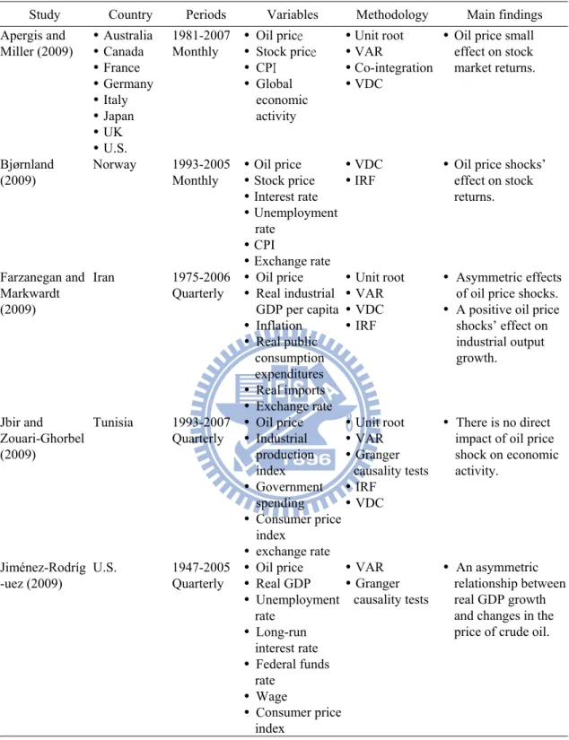
Table 2.1 An Overview of Previous Studies of the Impacts of Energy Price Shocks on Industrial Production and Macroeconomics Activities, 1999-2009.
Study Country Periods Variables Methodology Main findings Apergis and Miller (2009) Australia Canada France Germany Italy Japan UK U.S. 1981-2007 Monthly Oil price Stock price CPI Global economic activity Unit root VAR Co-integration VDC
Oil price small effect on stock market returns. Bjørnland (2009) Norway 1993-2005 Monthly Oil price Stock price Interest rate Unemployment rate CPI Exchange rate VDC IRF
Oil price shocks’ effect on stock returns. Farzanegan and Markwardt (2009) Iran 1975-2006 Quarterly Oil price Real industrial GDP per capita Inflation Real public consumption expenditures Real imports Exchange rate Unit root VAR VDC IRF Asymmetric effects of oil price shocks. A positive oil price
shocks’ effect on industrial output growth. Jbir and Zouari-Ghorbel (2009) Tunisia 1993-2007 Quarterly Oil price Industrial production index Government spending Consumer price index exchange rate Unit root VAR Granger causality tests IRF VDC There is no direct impact of oil price shock on economic activity. Jiménez-Rodríg -uez (2009) U.S. 1947-2005 Quarterly Oil price Real GDP Unemployment rate Long-run interest rate Federal funds rate Wage Consumer price index VAR Granger causality tests An asymmetric relationship between real GDP growth and changes in the price of crude oil.
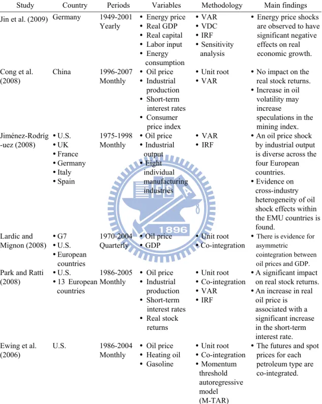
Table 2.1 An Overview of Previous Studies of the Impacts of Energy Price Shocks on Industrial Production and Macroeconomics Activities, 1999-2009 (Continued)
Study Country Periods Variables Methodology Main findings Jin et al. (2009) Germany 1949-2001
Yearly Energy price Real GDP Real capital Labor input Energy consumption VAR VDC IRF Sensitivity analysis
Energy price shocks are observed to have significant negative effects on real economic growth. Cong et al. (2008) China 1996-2007 Monthly Oil price Industrial production Short-term interest rates Consumer price index Unit root VAR No impact on the real stock returns. Increase in oil volatility may increase speculations in the mining index. Jiménez-Rodríg -uez (2008) U.S. UK France Germany Italy Spain 1975-1998 Monthly Oil price Industrial output Eight individual manufacturing industries VAR IRF
An oil price shock by industrial output is diverse across the four European countries. Evidence on cross-industry heterogeneity of oil shock effects within the EMU countries is found. Lardic and Mignon (2008) G7 U.S. European countries 1970-2004 Quarterly Oil price GDP Unit root Co-integration
There is evidence for asymmetric
cointegration between oil prices and GDP. Park and Ratti
(2008) U.S. 13 European countries 1986-2005 Monthly Oil price Industrial production Short-term interest rates Real stock returns Unit root Co-integration VAR IRF A significant impact on real stock returns. An increase in real oil price is associated with a significant increase in the short-term interest rate. Ewing et al. (2006) U.S. 1986-2004 Monthly Oil price Heating oil Gasoline Unit root Co-integration Momentum threshold autoregressive model (M-TAR)
The futures and spot prices for each petroleum type are co-integrated.
Table 2.1 An Overview of Previous Studies of the Impacts of Energy Price Shocks on Industrial Production and Macroeconomics Activities, 1999-2009 (Continued)
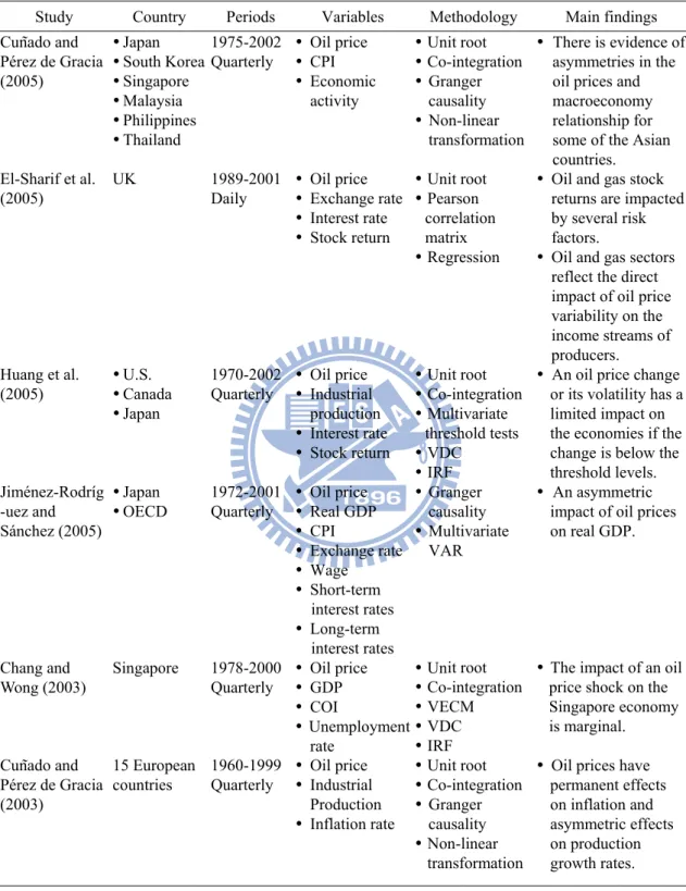
Study Country Periods Variables Methodology Main findings Cunado and Pérez de Gracia (2005) Japan South Korea Singapore Malaysia Philippines Thailand 1975-2002 Quarterly Oil price CPI Economic activity Unit root Co-integration Granger causality Non-linear transformation There is evidence of asymmetries in the oil prices and macroeconomy relationship for some of the Asian countries. El-Sharif et al. (2005) UK 1989-2001 Daily Oil price Exchange rate Interest rate Stock return Unit root Pearson correlation matrix Regression
Oil and gas stock returns are impacted by several risk factors.
Oil and gas sectors reflect the direct impact of oil price variability on the income streams of producers. Huang et al. (2005) U.S. Canada Japan 1970-2002 Quarterly Oil price Industrial production Interest rate Stock return Unit root Co-integration Multivariate threshold tests VDC IRF
An oil price change or its volatility has a limited impact on the economies if the change is below the threshold levels. Jiménez-Rodríg -uez and Sánchez (2005) Japan OECD 1972-2001 Quarterly Oil price Real GDP CPI Exchange rate Wage Short-term interest rates Long-term interest rates Granger causality Multivariate VAR An asymmetric impact of oil prices on real GDP. Chang and Wong (2003) Singapore 1978-2000 Quarterly Oil price GDP COI Unemployment rate Unit root Co-integration VECM VDC IRF
The impact of an oil price shock on the Singapore economy is marginal. Cunado and Pérez de Gracia (2003) 15 European countries 1960-1999 Quarterly Oil price Industrial Production Inflation rate Unit root Co-integration Granger causality Non-linear transformation
Oil prices have permanent effects on inflation and asymmetric effects on production growth rates. Notes: VDC denotes the variance decomposition; IRF denotes the impulse response functions.
Table 2.1 An Overview of Previous Studies of the Impacts of Energy Price Shocks on Industrial Production and Macroeconomics Activities, 1999-2009 (Continued)
Study Country Periods Variables Methodology Main findings Hamilton (2003) U.S. 1949-2001 Quarterly Oil price GDP Non-linear regression model
Oil price increases are much more important than oil price decreases. Sadorsky (2003) U.S. 1984-2000 Monthly Oil price Industrial production Interest rate Exchange rate CPI Unit root Ordinary least squares regression The conditional volatilities of oil prices, the term premium, and the consumer price index each have a significant impact on the conditional volatility of technology stock prices.
Balke et al. (2002) U.S. 1965-1997 Monthly Oil price GDP CPI Interest rate Unit root Quasi-VAR IRF Negative and positive oil price shocks have asymmetric effects on output and interest rates. Davis and Haltiwanger (2001) U.S. 1972-1988 Monthly Oil price Job creation rate Job destruction rate Employment growth rate
Panel VAR Oil shocks account for 20-25% of the variability in employment growth. Employment growth responds asymmetrically to oil price ups and downs. Papapetrou (2001) Greece 1989-1999 Monthly Oil price Stock return Industrial production Industrial employment growth rate Unit root Co-integration VDC IRF
Oil price changes affect economic activity and employment. Sadorsky (1999) U.S. 1947-1996 Monthly Oil price Stock return Interest rate Unit Root Generalised autoregressive conditional heteroskedastic (GARCH) model Oil price movements explain a larger fraction of the forecast error variance in real stock returns than do interest rates. Oil price volatility shocks have asymmetric effects on the economy. Notes: VDC denotes the variance decomposition; IRF denotes the impulse response functions.
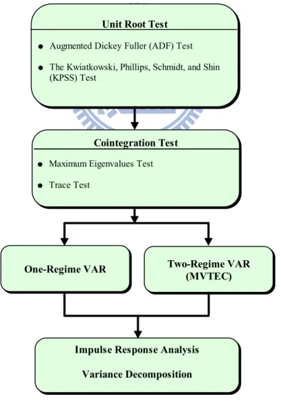
Chapter 3 Methodology
To more clearly express the econometric methodology, we outline the research process in Figure 3.1. The first step is to check the variables either stationarity or non-stationarity. The second step is to test the non-stationarity sequences are integrated of the same order and residual sequence is stationary. The traditional one-regime VAR model and the multivariate threshold error correction model will be introduced. Finally, impulse response function (IRF) and variance decomposition (VDC) track the dynamic relationship between macroeconomic variables within VAR models.
Cointegration Test
Maximum Eigenvalues Test Trace Test
Unit Root Test
Augmented Dickey Fuller (ADF) Test The Kwiatkowski, Phillips, Schmidt, and Shin (KPSS) Test
Two-Regime VAR (MVTEC) One-Regime VAR
Impulse Response Analysis Variance Decomposition
3.1 Unit Root Tests
Some economic or financial time series variables have non-stationary characteristic if the data generating process of time series variables have random walk. Therefore, the first step is to check the variables either stationarity or non-stationarity.
A time series is a set of y observations, each one being recorded at a specific t
time t with stochastic process. A stationary series can be defined as one with a constant mean, constant variance and constant autocovariances for each given lag. The stationarity or otherwise of a series can strongly influence its behavior and properties. A change or an unexpected change in a variable to the system will gradually die away.
On the other hand, a non-stationary series necessarily has permanent components. The mean and variance of non-stationary series are time-dependent and the sample correlogram dies away slowly in finite samples. There is no long-run mean to which the series returns.
According to Granger and Newbold (1974), the use of non-stationary data leads to spurious regression. Its result may have higher coefficient of determinant and much significant t value. If standard regression techniques are applied to non-stationary data, the result could be a regression that ‘looks’ good under standard measures (significant coefficient estimates and a high R2, but which is really valueless). There is a reason why the concept of non-stationarity is important and why it is essential that variables that are non-stationarity be treated differently from those that are stationarity. We adopt two applicable unit root methods for examining the existence of unit roots.
3.1.1 Augmented Dickey Fuller (ADF) Test
Dickey and Fuller (1979) consider a autoregressive process AR(1) model
1 1
t t t
y =a y− + , where the disturbances, ε εt, are assumed to be white noise, conditional on past y , and the first observation, t y , is assumed to be fixed. By subtracting 1 yt−1
from both sides of the equation, we can rewrite the model as follows: ∆ =yt γyt−1+ , εt where γ = − . The unit root test is equivalent to testinga1 1 γ = , that is, that there 0 exists a unit root. The standard t-statistic for γˆ can be used to testγ = , but with the 0 Dickey-Fuller critical values.
However, simple unit root test described above is valid only if the series is an AR(1) process. If the series is correlated at higher order lags, the assumption of white noise disturbances is violated. Dickey and Fuller (1981) make a parametric correction for higher order correlation by assuming that the
{ }
yt follows an AR(p) process and extending model as follows:0 1 1 2 2 1 1
t t t p t p p t p t
y =a +a y− +a y− + +… a y− − + +a y− +ε (1) By adding and subtracting a yp t p− +1 from both sides of the equation then the differenced form is:
0 1 1 2 2 2 2 ( 1 ) 1 1
t t t p t p p p t p p t p t
y =a +a y− +a y− + +… a − y− + + a − +a y− + − ∆a y− + +ε (2) Next, add and subtract (ap−1+a yp) t p− +2 to obtain:
0 1 1 2 2 ( 1 ) 2 1
t t t p p t p p t p t
y =a +a y− +a y− + −… a − +a ∆y− + − ∆a y− + +ε (3) Continuing in this fashion, we get:
0 1 1 2 p t t i t i t i y a γy− β y− + ε = ∆ = + +
∑
∆ + , (4) where 2 1 p i i a γ = ⎛ ⎞ = − −⎜ ⎟ ⎝∑
⎠ and p i j j i a β = =∑
In Eq. (4), the coefficient of interest isγ . If γ = , the equation is entirely in first 0 differences and so has a unit root. Three ADF test actually consider three different regression equations that can be used to test for the presence of a unit root:
1 1 2 p t t i t i t i y γy− β y− + ε = ∆ = +
∑
∆ + (5)0 1 1 2 p t t i t i t i y a γy− β y− + ε = ∆ = + +
∑
∆ +(6) 0 1 2 1 2 p t t i t i t i y a γy− a t β y− + ε = ∆ = + + +
∑
∆ + . (7) The differences between the three regressions concerns the presence of the deterministic elements a0 and a t2 . Without an intercept and time trend belongs in Eq. (5); with only the intercept belongs in Eq. (6); and with both an intercept and trend belongs in Eq. (7). If the coefficients of a difference equation sum to one, at least one characteristic root is unity. If Σ = and ai 1 γ = , the system has a unit root. 03.1.2 The Kwiatkowski, Phillips, Schmidt, and Shin (KPSS) Test
It is a well-established empirical fact that standard unit root tests fail to reject the null hypothesis of a unit root for most aggregate economic time series. In general, most of the standard unit root tests suffer from three problems. First, several approaches have severe size distortions when the moving average polynomial of the first differences series has a large negative autoregressive root (Schwert, 1989). Second, the testing statistics have low power when the root of the autoregressive polynomial is close to unity (DeJong et al., 1992; Kwiatkowski et al., 1992). Third, conducting the unit root tests often implies the selection of an autoregressive truncation lag, k, which is strongly related to the size distortions and the extent of power loss (Ng and Perron, 1995). Many studies (DeJong et al., 1989; Diebold and Rudebusch, 1991; DeJong and Whiteman, 1991; Phillips, 1991) suggest that, in trying to decide by classical methods whether economic data are stationary or integrated, it would be useful to perform tests of the null hypothesis of stationarity as well as tests of the null hypothesis of a unit root. The Kwiatkowski, Phillips, Schmidt, and Shin (KPSS) test provides a straightforward test of the null hypothesis of stationarity against the alternative of a unit root.
Kwiatkowski et al. (1992) propose a test of the null hypothesis that an observable series is stationary around a deterministic trend. The series is expressed as the sum of deterministic trend, random walk, and stationary error, and the test is the LM test of the hypothesis that the random walk has zero variance. The KPSS statistic is based on the residuals from the OLS regression of yt on the exogenous variablesxt:
t t t y =x′δ ε+
The Lagrange Multiplier (LM) statistic can be defined as:
2 2 1 ˆ / T t t LM S σε = =
∑
,where S is a cumulative residual function (i.e., t
1 ˆ , 1, 2, , t t i i S ε i T = =
∑
= … ). We pointout that the estimator of δ used in this calculation differs from the estimators for δ used by detrended GLS since it is based on a regression involving the original data and not on the quasi-differenced data. Finite sample size and power are considered in a Monte Carlo experiment.
Prior to performing the Johansen co-integration method, we need to determine the appropriate number of lag length of the VAR model. The Bayesian information criterion (BIC) (Schwarz, 1978) is employed. The test criteria to determine appropriate lag lengths and seasonality are the multivariate generalizations of the BIC. The BIC criterion is a purely statistical technique and allows data themselves to select optimal lags. Given any two estimated models, the model with the lower value of BIC is the one to be preferred. The selection of lag order of ∆yt i− can be used by the Bayesian information criterion (BIC):
BIC=-2*ln(L)+k*ln(n) (8)
where n is the number of observations, k is the number of free parameters to be estimated and L is the maximized value of the likelihood function for the estimated model. The BIC penalizes free parameters more strongly than does the Akaike
information criterion (AIC) (Akaike, 1969).
3.2 Cointegration Analysis
The co-integration theory is defined that a linear combination of non-stationary variables is stationary (Engle and Granger, 1987). Although the Engle and Granger (1987) procedure is easily implemented, it does have two important defects. The first one is that such method has no systematic procedure for the separate estimation of the multiple cointegrating vectors. Another serious defect of the Engle and Granger (1987) procedure is that it relies on a two-step estimator. The coefficient a is obtained by 1
estimating a regression using the residuals from another regression. The error terms introduced by the researcher in first step is carried into second step. Fortunately, the Johansen co-integration method has been developed and can avoid two problems.
The Johansen co-integration method is provided by Johansen (1988) and Johansen and Juselius (1990). This procedure applying maximum likelihood estimators circumvent the low-power of using Granger two-step estimators and can estimate and test for the presence of multiple cointegrating vectors. Moreover, this test allows the researcher to test restricted versions of the cointegrating vectors and speed of adjustment parameters.
Let yt denotes the (n× vector1) (y y1 , 2 ,t t...,ynt). The maintained hypothesis is that y follows a VAR(P) in levels and all of the elements for t y are I(1) process. t
1 +A2 + +Ap + ,t 1, 2, , A ε t T = = t t-1 t-2 t-p y y y … y … (9) where εti i d. . .∼ N(0, )Ω .
Eq. (10) can be put in a more usable form by subtracting yt−1 from each side to obtain:
1 2
(A I) +A + +Ap + ,εt t 1, 2, ,T
Now add and subtract (A1−I)y to obtain: t-2
1 2 1
(A I) +(A A I) + +Ap + ,εt t 1, 2, ,T
∆ =yt − yt-1 + − yt-2 … yt-p = … (11)
Continuing in this fashion, we obtain: 1 1 p t i π π ε − = ∆ =yt
∑
∆yt-i+ ∆yt-p+ (12) where 1 p i i I A π = ⎛ ⎞ = −⎜ − ⎟ ⎝∑
⎠ 1 i i j j I A π = ⎛ ⎞ = −⎜ − ⎟ ⎝∑
⎠Suppose we obtained the matrix π and order the n characteristic roots such thatλ λ1> 2 > > . If the variables in ... λn y are not cointegrated, the rank of t π is
zero and all these characteristic roots will equal zero. Similarly, since ln(1) 0= , each of the expressions ln(1−λi) will equal zero if the variables are not cointegrated.
Suppose that each individual variable y is it I(1) and linear combinations of y t
are stationary. That implies π can be shown as
π αβ= ′
where β is the matrix of cointegrating parameters, and α is the matrix of the speed of adjustment parameters. The number of cointegrating relations relies on the rank of π , and the rank of π is:
(1) rank( ) nπ = , λ is full rank means that all components of y is a stationary t
process.
(2) rank( ) 0π = , λ is null matrix meaning that there is no cointegration relationships. (3) 0 rank( ) r n< π = < , the variables for y are cointegrated and the number of t
cointegrating vectors is r.
The test for the number of characteristic roots that are insignificantly different from unity can by conducted using the following two test statistics:
(1) Trace test: 1 ˆ ( ) n ln(1 ) trace i i r r T λ λ = + = −
∑
− , 0: rank( ) H π ≤ , r 1: rank( ) H π > rwhere λˆi is the estimated values of the characteristic roots (also called eigenvalues) obtained from the estimated π matrix, r is the cointegrating vector, and T is the
number of usable observations. The statistic tests the null hypothesis that the number of distinct cointegrating vectors is less than or equal to r against a general alternative. If there is no cointegrating vector, it should be clear that λtrace equals zero when allλˆi =0. The further the estimated characteristic roots are from zero, the more negative is ln(1−λˆi) and the larger the λtrace statistic.
(2) Maximum eigenvalues test: max( ,r r 1) Tln(1 ˆr 1)
λ + = − −λ+
0
H : there are r cointegrating vectors
1
H : there are r+ cointegrating vectors 1
The statistic tests the null that the number of cointegrating vectors is r against the alternative of r+ cointegrating vectors. If the estimated value of the characteristic 1 root is close to zero, λmax will be small. The critical values of the λtrace and λmax statistics follows a chi-square distribution in general.
3.3 Multivariate Threshold Error Correction (MVTEC) Model
The threshold autoregressive (TAR) model is first developed by Tong (1978). The TAR model assumes that different regimes can be determined based on the threshold variable. Hence, TAR models in which the process is piecewise linear in the
threshold space. Tsay (1998) generalizes the univariate threshold principle of Tsay (1989) to a multivariate framework. He use predictive residuals to construct a test statistic for detecting threshold nonlinearity in a vector time series and propose a procedure for building a multivariate threshold model.
At the beginning, we consider the univariate TAR model which is also referred to as SETAR (self-exciting TAR). The SETAR(1) can be formed as:
0,1 1,1 1 1 0,2 1,2 1 1
yt =(φ +φ y )(1t− −I z[ t− >c]) (+ φ +φ y ) [t− I zt− > + (13) c] εt where εt is a white noise process, zt−1= yt−1, and c represents the threshold value.
( )
I ⋅ is an index function, which equals to one if the relation in the brackets holds, and equals to zero otherwise. Eq. (13) can be treated as a multivariate threshold VAR(1). Consider a k-dimensional time series yt =( , ,y1t … y ′kt) and assume there is a cointegration relationship among these variables, then yt follows a multivariate threshold error correction model (MVTEC) with threshold variable z and delay d and t
can be expressed as:
1 1 1 ,1 1 2 2 1 ,2 1 ( )(1 [ ]) ( ) [ ] (14) p t i t d i p t i t d t i I z c I z c α β θ φ α β θ φ ε − − = − − = = + + − > + + + > +
∑
∑
t t-i t-i y y ywhere α1 and α2 are the constant vectors below and above the threshold value, respectively. p and d are the lag length of y and delay order of t z , respectively. t
Both p and d are nonnegative integers. θt−1 is an error correction term. The threshold variable is assumed to be stationary and have a continuous distribution. Model (14) has two regimes and is a piecewise linear model in the threshold space zt d− .
Given observations
{
yt, zt}
, wheret= … , we have to detect the threshold 1, ,nnonlinearity ofy . Assuming p and d are known, the Eq. (14) can be re-written as: t
Xt εt, t h 1, ,n
′ = Φ +′ ′ = +
t
where max( , )h= p d , Xt =(1, y ,′t−1 …y ,tt p′−− θt−1)′ is a (pk+ -dimensional regressor, 1) and Φ denotes the parameter matrix. If the null hypothesis holds, then the least squares estimates of (15) are useful. On the other hand, the estimates are biased under the alternative hypothesis. Eq. (15) remains informative under the alternative hypothesis when rearranging the ordering of the setup. For Eq. (15), the threshold variable zt d− assumes values in S =
{
zh+ −1 d,…zn d−}
. Consider the order statistics ofS and denote the ith smallest element of S by z . Then the arranged regression based ( )i
on the increasing order of the threshold variable zt d− is
( ) ( )
Xt i d+ εt i d+ , i 1, ,n h
′ = ′ + ′ = −
t(i)+d
y Φ … , (16) where ( )t i is the time index of z . Tsay (1998) use the recursive least squares ( )i
method to estimate (16). If y is linear, then the recursive least squares estimator of t
the arranged regression (16) is consistent, so the predictive residuals approach white noise. Consequently, predictive residuals are uncorrelated with the regressor Xt i d( )+ .
Let Φm be the least squares estimate of Φ of Eq. (16) with i= …1, ,m; i.e., the
estimate of the arranged regression using data points associated with the m smallest values of zt d− . Tsay (1998) suggests a range of m (between 3 n and 5 n ). Different values of m can be used to investigate the sensitivity of the modeling results with respect to the choice. It should be noted that the ordered autoregressions are sorted by the variablezt d− , which is the regime indicator in the MVTEC model. Let
( 1) ˆ ( 1) ˆet m′ + +d =yt(m+1)+d-Φ′ ′µXt m+ +d (17) and 1/ 2 ( 1) ( 1) ( 1) ( 1) ˆt m d ˆet m d / 1 Xt m dV Xm t m d η + + = + + ⎡⎣ + ′ + + + + ⎤⎦ , (18)
where V = m1X( ) X( ) 1
m i t i d t i d
−
= + ′ +
⎡Σ ⎤
⎣ ⎦ is the predictive residual and the standardized
predictive residual of regression (16). These quantities can be efficiently obtained by the recursive least squares algorithm. Next, consider the regression
( ) ( ) ( ) 0
ˆt l d Xt l d wt l d, l m 1, ,n h
η + = ′ + Ψ + ′ + = + … − , (19) where m denotes the starting point of the recursive least squares estimation. The 0
problem of interest is then to test the hypothesis H0:Ψ = versus the alternative 0
1: 0
H Ψ ≠ in regression (19). The ( )C d statistic is therefore defined as:
{
1}
( ) ( 1) ln So ln S
C d = n p m kp− − − − × − , (20) where the delay d implies the test depends on the threshold variable zt d− , and
0 ( ) ( ) 1 0 1 ˆ ˆ So n h t l d t l d l m n h m η η − + + = + ′ = − −
∑
and 0 1 ( ) ( ) 1 0 1 ˆ ˆ S n h wt l dwt l d l m n h m − + + = + ′ = − −∑
,where ˆwt is the least squares residual of regression (19). Under null hypothesis the yt is linear and some regularity conditions, C(d) is asymptotically a chi-squared random variable with (k pk+ degree of freedom. 1)
3.4 Impulse Response Analysis
Impulse response function (IRF) tracks the dynamic relationship between macroeconomic variables within VAR models. It is an essential tool in empirical causal analysis and policy effectiveness analysis. In applied work it is often of interest to know the response of one variable to an impulse in another variable in a system that involves a number of other variables as well, or how long these effects require to take place. By imposing specific restrictions on the parameters of the VAR model the shocks can be attributed an economic meaning.