利用快取增加IPv6下的封包分類效能

全文

(1)利用快取增加 IPv6 下的封包分類效能 Performance Improvement of Packet Classification with Caching for IPv6. 研究生：何凱元. Student：Ho Kai-Yuan. 指導教授：陳耀宗博士. Advisor：Dr. Yaw-Chung Chen. 國立交通大學資訊工程系碩士論文. A Thesis Submitted to Department of Computer Science and Information Engineering College of Electrical Engineering and Computer Science National Chiao Tung University in partial Fulfillment of the Requirements for the Degree of Master in Computer and Information Science June 2004 Hsinchu, Taiwan, Republic of China. 中華民國九十三年六月 i.

(2) 利用快取增加 IPv6 下的封包分類效能研究生：何凱元. 指導教授：陳耀宗博士. 國立交通大學資訊工程學系中文摘要封包分類技術，是將封包依照其標頭的內容，將封包分類成不同的類別。封包分類目前應用在網路安全、網路服務分級、路由搜尋、流量分散等項目上。而目前的封包分類方式，可分為軟體及硬體實做兩種。而目前大部分的封包分類方式，在網路環境升級成 IPv6 後，由於標頭內容大幅增長，使得分類效能下降，整體網路效能大幅下滑。在本篇論文中，我們提出使用快取方式，來增進封包分類在 IPv6 下的效率。我們對不同的快取記憶體容量、記憶體架構、以及快取內容的替換選擇方式等項目做了測試。在我們的實驗中，當快取記憶體的大小為 1024 格的情形下，快取的命中率可以達到 9 成以上，大幅增加封包分類的效率。. ii.

(3) Performance Improvement of Packet Classification with Caching for IPv6. student：Ho Kai-Yuan. Advisors：Dr. Yaw-Chung Chen. Department of Computer Science and Information Engineering National Chiao Tung University ABSTRACT Packet classification is a technique that classifies flows into different class by the headers in packets. Packet classification is applied in network security, QoS, routing, load balancing, and etc. Currently, algorithms of packet classification are categorized into hardware or software solutions. Almost packet classification implementations can not be efficient enough when the network environment is upgraded to IPv6 because the much longer fields in the header. In this thesis, we proposed that use a cache memory to improve performance of packet classification in IPv6. We also simulated the performance under different cache sizes, architectures, replacement policies, and etc. According to the simulations, our schemes can achieve hit rates more than 90% when cache size is more than 1024 in 4-way associative cache memory architecture.. iii.

(4) Table of Contents 中文摘要 .........................................................................ii ABSTRACT................................................................... iii Table of Figures and Tables ............................................vi CHAPTER 1 INTRODUCTION .....................................1 CHAPTER 2 BACKGROUND .......................................3 2.1 Related work......................................................................................3. CHAPTER 3 RANDOM BIT-SELECTION ...................4 3.1 Overview ...........................................................................................4 3.2 Sample of traffic data ........................................................................4 3.3 Range of selection .............................................................................6 3.3.1 shortened protocol number ...........................................................................7. 3.4 Preparation for experiment................................................................7. CHAPTER 4 CACHE ARCHITECTURE FOR IPV6 HEADER CACHING ......................................................8 4.1 Overview ...........................................................................................8 4.2 The structure of cache memory .........................................................8 4.2.1 Parameters of cache memory ........................................................................8 4.2.2 Fields in cache memory ................................................................................9. 4.3 Replacement policies.......................................................................10 4.3.1 LRU.............................................................................................................10 4.3.2 LFU .............................................................................................................10 4.3.3 Random .......................................................................................................10. 4.4 Associativity ....................................................................................11 4.4.1 Full associativity ......................................................................................... 11 4.4.2 N-way associativity..................................................................................... 11. 4.5 Hash functions.................................................................................12 4.5.1 Hash function I............................................................................................12 iv.

(5) 4.5.2 Hash function II ..........................................................................................13 4.5.3 Hash function III .........................................................................................14 4.5.4 Collision analysis ........................................................................................15. 4.6 Dealing with rule updates................................................................15. CHAPTER 5 MEASUREMENTS.................................16 5.1 Simulation of random bit-selection .................................................16 5.1.1 Experimental procedure ..............................................................................16 5.1.2 Types of range.............................................................................................16 5.1.3 Experimental result .....................................................................................16. 5.2 Simulation of IPv6 header caching .................................................21 5.2.1 Miss ratios...................................................................................................21 5.2.2 Misclassification ratios ...............................................................................24 5.2.3 Hardware complexity..................................................................................26. CHAPTER 6 CONCLUSIONS .....................................27 CHAPTER 7 FUTURE WORK.....................................28 7.1 IPv6 protocol chain problem ...........................................................28 7.2 Special layer-4 protocol processing ................................................28 7.3 Use of flow label .............................................................................29. REFERENCES ..............................................................30. v.

(6) Table of Figures and Tables Table 3.1 Analysis of sample 1 and sample 2…………………..5 Figure 3.1 Analysis of traffic samples (in packets)…………….5 Figure 3.2 Analysis of traffic samples (in flows)……………….6 Figure 4.1 Structure of a Cache entry…………………………..9 Figure 4.2 Hash function I.…………………………………....13 Figure 4.3 Hash function III…………………………………..14 Table 4.1 Collision analysis of the three hash functions………15 Table 5.1 Random bit-selection evaluation on sample 1 (number of collisions)…………………………………………………..18 Table 5.2 Random bit-selection evaluation on sample 1 (in collision ratios)………………………………………………..18 Figure 5.1 Random bit-selection evaluations on sample 1……19 Table 5.3 Random bit-selection evaluation on sample 2 (number of collisions)…………………………………………………..19 Table 5.4 Random bit-selection evaluation on sample 2 (in collision ratios)………………………………………………..20 Figure 5.2 Random bit-selection evaluations on sample 2……20 Table 5.5 Miss rates with different replacement policies and vi.

(7) associativities (# of entries=65536)…………………………...22 Figure 5.3 Miss times with different replacement policies and associativities (# of entries=65536)…………………………...22 Table 5.6 Miss Rates with different associativities and cache sizes (Replacement policy: LRU)……………………………..23 Figure 5.4 Miss Ratios with different associativities and cache sizes (Replacement policy: LRU)……………………………..23 Figure 5.5 Miss ratios with different replacement policies and cache sizes (Replacement policy: LRU)………………………24 Table 5.7 Misclassification ratios with different replacement policies and associativities (# of entries=65536)……………...25. vii.

(8) CHAPTER 1 INTRODUCTION There are a number of services that required packet classification, such as access control of firewall, QoS (Quality of Service), DiffServ (Differentiated quality of Service), and policy based routing. The packet classification process determines which flow a packet belongs to based on one or more fields in the packet header. Performance of packet classification affects the network throughput very obviously. With increasing speed of current network environment, for decreasing packet sizes of some real time network applications such as online games, it is very important to deliver high speed and low latency packet classification functionality at low cost. The problem of packet classification is a generalization of the one-dimensional IP route lookup problem, but is much harder and requires much more resources to perform. It has been well established that memory access delays limit the classification speeds. As memory speeds have not kept pace with the rest of the hardware advances, classification speeds are limited by memory access latency. Memory access latencies are about 50 to 60 ns in DRAM, 5 to 20 ns in SRAM, and 1 to 2 ns in on-chip SRAM. Even with on-chip SRAM to store the classification table, the classification process can only afford about 4 memory lookups at 40Gbps. To be compatible with current high speed network, we have an idea of caching the recently matched flows. The process of packet classification must be executed 1.

(9) only on a cache miss. Cost of cache is reasonable, and cache has been widely used in modern computer architecture for many years. In this thesis, we try to evaluate cache performance with real IPv6 traffic, and we propose hash functions to compress IPv6 flow ID in order to save cache space. Finally, we evaluate miss rate and misclassification rate for our hash function.. 2.

(10) CHAPTER 2 BACKGROUND 2.1 Related work We identify a flow by the 5-tuple: <Source Address, Destination Address, Source Port, Destination Port, Protocol>. We call the 5-tuple <SA, DA, SP, DP, protocol> “Flow ID”. Source and destination addresses in IPv4 are 32-bit long. But in IPv6, the fields are 128-bit long. Source and destination ports are 16-bit long, and protocol is 8-bit long. A flow ID is 104-bit long in IPv4, 296-bit long in IPv6. There have been a number of related studies in this area. Recent studies show that the arrival of a packet on an Internet link implies a very high probability of the arrival of another packet with the same flow identifier. Various packet classification algorithms have been proposed in the last few years, and Gupta et. al presented a survey for various classification algorithms. Studies for packet classifications based on flow identifier show similar improvement as route lookup by using a cache. Our studies differ from the above and we focus on the following: 1.Cache performance for IPv6 protocol 2.Hash functions for representation of IPv6 flow ID. 3.

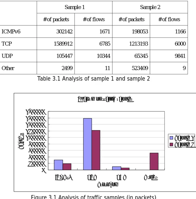
(11) CHAPTER 3 RANDOM BIT-SELECTION 3.1 Overview Random bit-selection is a simple hash function to generate variable-length bit string. Random bit-selection can be implemented simply with hardware lines, and its time complexity is constant.. 3.2 Sample of traffic data There is still too few IPv6 traffic available, so we use the traffic data provided by MAWI Working Group. MAWI (Measurement and Analysis on the WIDE Internet) Working Group Traffic Archive (http://tracer.csl.sony.co.jp/mawi/) is a working group that has carried out network traffic measurement, analysis, evaluation, and verification from the beginning of the WIDE Project. The WIDE Project carries out research activities through the use of the actual network, but simply operating the network alone does not qualify as research. The traffic samples were captured by tcpdump in binary format of tcpdump. We use the sample of the date 2004/03/13 from WIDE-Bone6 as sample 1. There are 2 million packets, 3507 distinct addresses, 18811 distinct flows in the sample 1. We also use the sample of the 2004/05/18 from 6Bone as sample 2. There are 2 million packets, 2518 distinct addresses, 17016 distinct flows in the sample 2. The default buffer size setting in tcpdump was too small to recognize all IPv6 extension headers. So some packets with IPv6 extension headers were recognized as “Other” protocol.. 4.

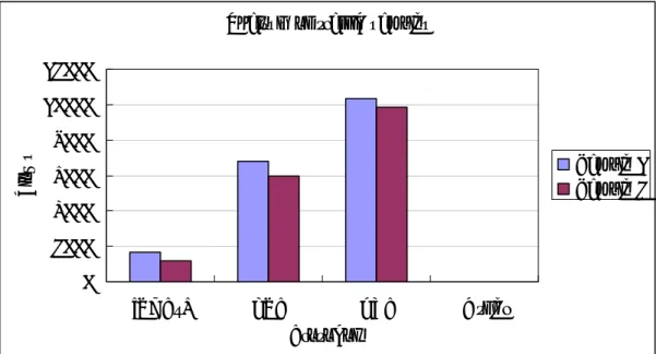
(12) Analysis data of the 2 samples is listed in Table 3.1, Figure 3.1 and 3.2.. Sample 1 # of packets ICMPv6. Sample 2. # of flows. # of packets. # of flows. 302142. 1671. 198053. 1166. TCP. 1589912. 6785. 1213193. 6000. UDP. 105447. 10344. 65345. 9841. Other. 2499. 11. 523409. 9. Table 3.1 Analysis of sample 1 and sample 2. Packets. Analysis of traffic samples 1800000 1600000 1400000 1200000 1000000 800000 600000 400000 200000 0. Sample 1 Sample 2. ICMPv6. TCP. UDP. Other. Protocol. Figure 3.1 Analysis of traffic samples (in packets). 5.

(13) Analysis of traffic samples 12000 10000. Flows. 8000 Sample 1 Sample 2. 6000 4000 2000 0 ICMPv6. TCP. UDP. Other. Protocol. Figure 3.2 Analysis of traffic samples (in flows). 3.3 Range of selection In order to improve the efficiency of random bit-selection, we have to determine the range of selection that is representative. Because the IPv6 addresses can be separated into two parts as prefix and MAC, we can use only one part in our random bit-selection to simplify the process of selection and shorten the execution time of simulation. We designed 5 types of range for random bit-selection. The types of range are listed below: Type 1: Prefixes of SA/DA, SP, DP, protocol (168 bits) Type 2: Full SA/DA, SP, DP, protocol (296 bits) Type 3: Full SA/DA, SP, DP, but no protocol (288 bits) Type 4: Prefixes of SA/DA, SP, DP, but no protocol (160 bits) Type 5: MAC parts of SA/DA, SP, DP, shortened protocol number (162 bits). 6.

(14) 3.3.1 shortened protocol number There are only 3 major layer-4 protocols in IPv6: ICMPv6, TCP, and UDP. We represent the protocols as 0,1, and 2 instead of original protocol number. In order to reduce meaningless bits in our selection, shortened protocol number is useful.. 3.4 Preparation for experiment To simplify the experiment, we convert the original binary traffic samples to human readable tcpdump text format. And, to collect the flow ID from the samples, we convert the tcpdump text format to another text file with a simple program written in Perl. The two steps simplify the traffic data and save disk space. Evaluation programs also can be simplified because of the simplified traffic data.. 7.

(15) CHAPTER 4 CACHE ARCHITECTURE FOR IPV6 HEADER CACHING 4.1 Overview IPv6 is the next-generation layer-3 protocol in the Internet. One of the main features of IPv6 is the 128-bit long IP address with extension headers. The address fields in IPv6 are 4 times as long as IPv4. The longer fields make the whole processing time longer. So, packet classification will be one of the performance bottlenecks in IPv6 environment because of the longer IP address. The fastest method of packet classification is by using a Ternary CAM (TCAM) that uses a linear amount of parallelism to match flows in constant time. But TCAMs are expensive, and updates to the CAM are slow. To place 128-bit addresses in TCAMs is also very tricky. So, we have an idea of caching the recently matched flows. Cost of cache memory is reasonable. Cache memory is also widely used in current computer architecture.. 4.2 The structure of cache memory 4.2.1 Parameters of cache memory There are three major parameters of cache memory: number of entries, associativity, and replacement policy. Total size of the cache memory is proportional to number of entries. Associativity decides the number of candidates when 8.

(16) replacement occurs. Replacement policy decides the method to choose a victim to be replaced. All the three major parameters affect the performance of cache memory and hardware complexity.. 4.2.2 Fields in cache memory. Index. TS/Counter. Tag. Result. Figure 4.1 Structure of a Cache entry Index: Position of the entry in the memory. Length of index is variable with the number of entries and associativity. Index is generated by a variable-length hash function such as random bit-selection. Length of index = log2(Number of entries/Associativity) This is between 1 and 4, for associativity. Tag: A checksum-like field to check whether the two flows are identical. Tag is generated by a hash function and must be independent of index to avoid misclassification. When the index and tag fields of two flows are the same, they are judged to be identical. Length of tag is 32-bit. TS/Counter: Recent access record of this entry. The meaning of this field is decided by the replacement policy. For LRU, this field is used to store recent access time represented as a timestamp (TS); for LFU, it is used to count recent access times. Length of TS or counter is determined by the range of timestamp (LRU) or the maximum value of counter (LFU). If the associativity is direct-mapping or full associativity, or replacement policy is random, this field can be ignored. Result: The rule number or action for this flow. Length of result is determined by the range of rule number, or number of possible actions.. 9.

(17) By the way, valid bit is not necessary. If all fields of an entry are zero, the entry is accepted as invalid. So we reset the cache memory in initialization.. 4.3 Replacement policies 4.3.1 LRU LRU=Least Recently Used, the entry with oldest last accessed time will be replaced. Each cache entry includes a field called timestamp (TS) to record the last access time of this entry. To simplify the TS field, we use a 32-bit packet serial number instead of original floating-point number timestamp. Entry with oldest serial number will be replaced.. 4.3.2 LFU LFU=Least Frequently Used, the entry with least accessed count will be replaced. Each cache entry includes a small counter. Cache hits on an entry increment the entry’s counter up to a certain limit. Cache miss decrements the counter down to zero. The victim is chosen with the value in counter field. Entry with least counter value will be replaced.. 4.3.3 Random The victim to be replaced is randomly chosen. We use a random number generator to generate an integer number between 0 and associativity N-1, and the victim is decided by the generated random number. There is no extra field such as timestamp or counter needed for random replacement. 10.

(18) 4.4 Associativity The number of candidates to be replaced depends on the associativity. Associativity is an important parameter for cache memory because it affects the practical performance and hardware complexity.. 4.4.1 Full associativity In full associativity, all the entries in the cache memory are candidates. The performance of full associativity is already known as best, but the hardware cost is very high because a large amount of logic gates are needed to compare in parallel. In full associativity, index field is ignored when matching a flow or replacing an entry.. 4.4.2 N-way associativity In N-way associativity, the number of candidates to be replaced is equal to N. When N equals to 1, it is called directed-mapping. Because there is only one candidate to be replaced in direct-mapping, the replacement policy does not affect the result.. 11.

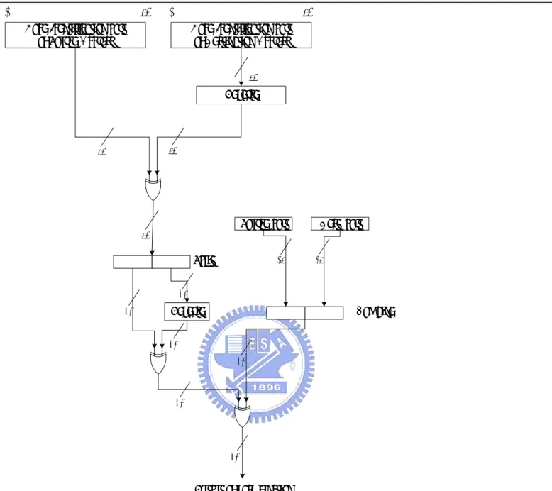
(19) 4.5 Hash functions We designed three hash functions to generate the field “Tag” in cache memory. We also tested the three hash functions with the two traffic samples.. 4.5.1 Hash function I The figure of hash function I is shown as Figure 4.2. The protocol field is ignored in ours hash functions. If the layer-4 protocol is neither TCP nor UDP, we set the source port and destination port number to zero. The hash function can be implemented directly with XOR gates, combine function, split function, and reverse function. Reverse, split and combine function can be simply implemented with only hardware lines. So the total delay of hash function I is three times XOR gate delay.. 12.

(20) 1. 64. 1. 64. Node Identification part of Source Address. Node Identification part of Destination Address 64. Reverse. 64. 64. Source port. Dest. port. 64. Split. 16. 16. 32 32. Reverse. Combine. 32 32. 32. 32. Output of hash function. Figure 4.2 Hash function I. 4.5.2 Hash function II The hash function II is very similar to I, but the port number will be set to 65535 if layer-4 protocol is neither TCP nor UDP. So the figure of hash function II is omitted.. 13.

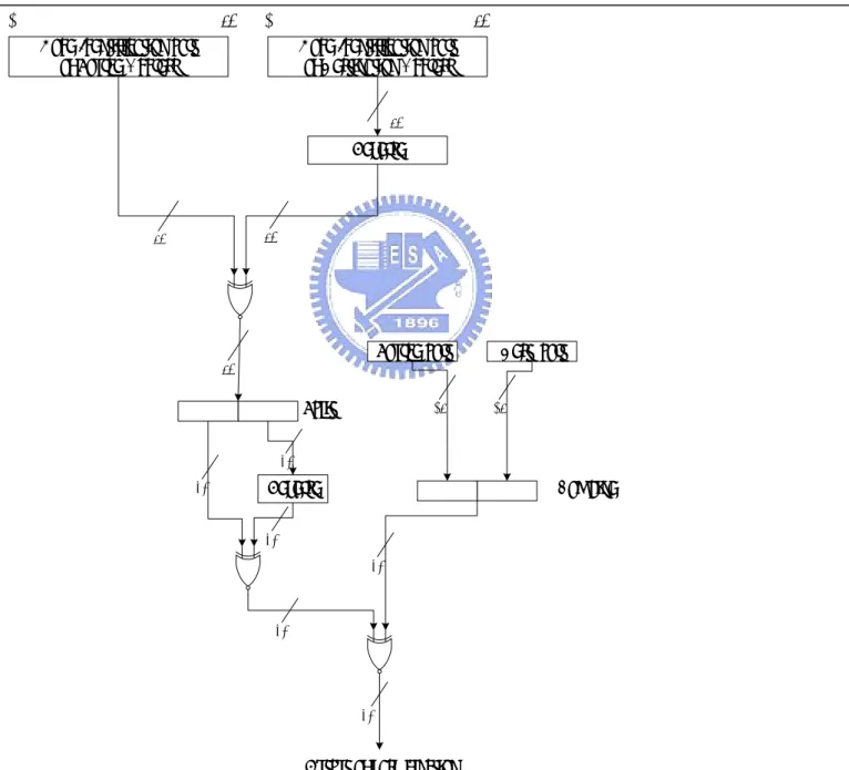
(21) 4.5.3 Hash function III The figure of hash function III is shown in Figure 4.3. The hash function III is similar to I and II, but the XOR gates in II are replaced with XNOR gates. Same as II, port number will be set to 65535 if layer-4 protocol is neither TCP nor UDP. So the total delay of hash function III is three times XNOR gate delay.. 1. 64. 1. 64. Node Identification part of Source Address. Node Identification part of Destination Address 64. Reverse. 64. 64. Source port. Dest. port. 64. Split. 16. 16. 32 32. Reverse. Combine. 32 32. 32. 32. Output of hash function. Figure 4.3 Hash function III 14.

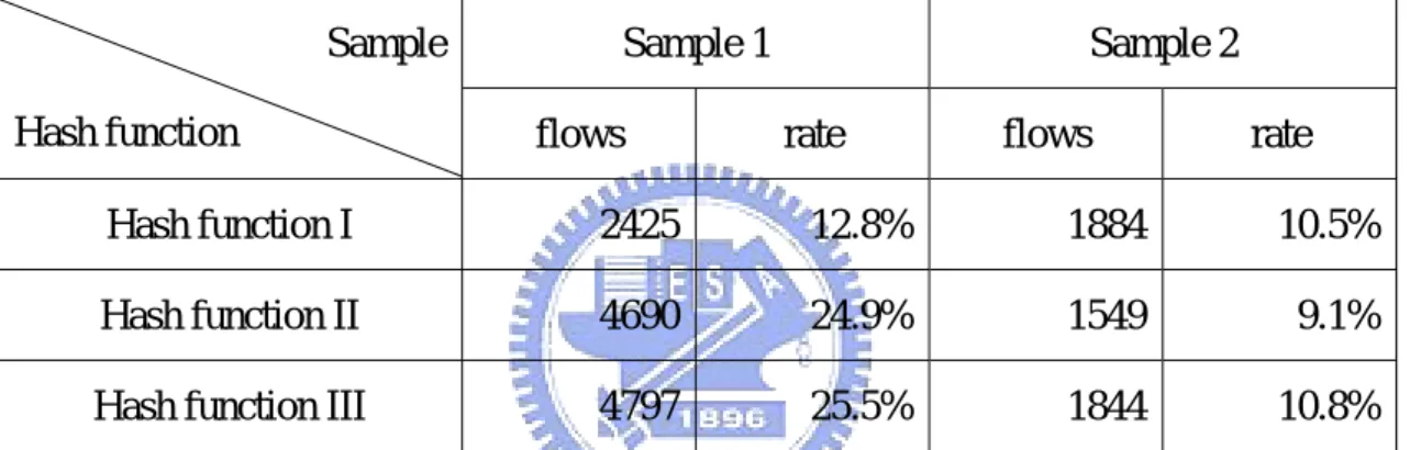
(22) 4.5.4 Collision analysis We evaluated the three hash functions with the 2 traffic samples. The collision rates should be as low as possible to avoid misclassification. Evaluation results are listed in Table 4.1. From Table 4.1, collision rates of hash function II and III are much higher than I for sample 1. But collision rates of the three functions for sample 2 are quite similar. So we suggest using hash function I to get low collision rate for both samples.. Sample Hash function. Sample 1 flows. Sample 2 rate. flows. rate. Hash function I. 2425. 12.8%. 1884. 10.5%. Hash function II. 4690. 24.9%. 1549. 9.1%. Hash function III. 4797. 25.5%. 1844. 10.8%. Table 4.1 Collision analysis of the three hash functions. 4.6 Dealing with rule updates Issues of rule update are rarely discussed in packet classification speedup skills. We recommend storing rule number instead of rule action in result field. For updates to the prefix or port number of a rule numbered X, cache entries with rule number X should be cleared to avoid inconsistency. For updates to the action of a rule numbered X, entries with rule number X should not be changed.. 15.

(23) CHAPTER 5 MEASUREMENTS. 5.1 Simulation of random bit-selection 5.1.1 Experimental procedure. Our experimental procedures are described as follows: 1. Translate the original binary traffic sample to text format with tcpdump. 2. Extract the essential fields from the text format sample to another file. 3. Compute the collision times, number of address, and number of flows from the extracted file.. 5.1.2 Types of range In order to optimize the performance of random bit-selection, the ranges of selection should be chosen carefully. The types of range are listed below: Type 1: Prefixes of SA/DA, SP, DP, protocol Type 2: Full SA/DA, SP, DP, protocol Type 3: Full SA/DA, SP, DP, but no protocol Type 4: Prefixes of SA/DA, SP, DP, but no protocol Type 5: MAC parts of SA/DA, SP, DP, shortened protocol number. 5.1.3 Experimental result. 16.

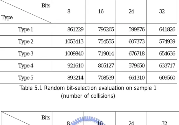
(24) For sample 1, the collision rates are between 55% and 29%. If the length is 24 or 32-bits long, type 2 is the best choice. If the length is 8 or 16-bits long, type 5 is the best choice. There is only a little difference when the length of random bit selection is 32. For sample 2, the collision rates are between 17% and 6%. If the length is 24 or 32-bits long, type 2 is the best choice. If the length is 8 or 16-bits long, type 5 is the best choice. From the result, the differences between the types are relatively small. We can just use any one of the types if the difference is neglectable. Smaller ranges, such as type 1, 3, 4, and 5, can simplify the hardware design and shorten the simulation time.. 17.

(25) Bits 8. 16. 24. 32. Type 1. 861229. 796265. 599876. 641826. Type 2. 1053413. 754555. 607373. 574939. Type 3. 1009840. 719014. 676718. 654636. Type 4. 921610. 805127. 579650. 633717. Type 5. 893214. 708539. 661310. 609560. Type. Table 5.1 Random bit-selection evaluation on sample 1 (number of collisions). Bits 8. 16. 24. 32. Type Type 1. 43.1%. 39.8%. 30.0%. 32.1%. Type 2. 52.7%. 37.7%. 30.4%. 28.7%. Type 3. 50.5%. 36.0%. 33.8%. 32.7%. Type 4. 46.1%. 49.3%. 29.0%. 31.7%. Type 5. 44.7%. 35.4%. 33.1%. 30.5%. Table 5.2 Random bit-selection evaluation on sample 1 (in collision ratios). 18.

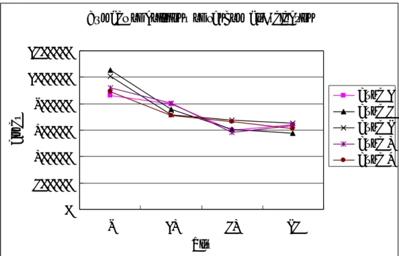
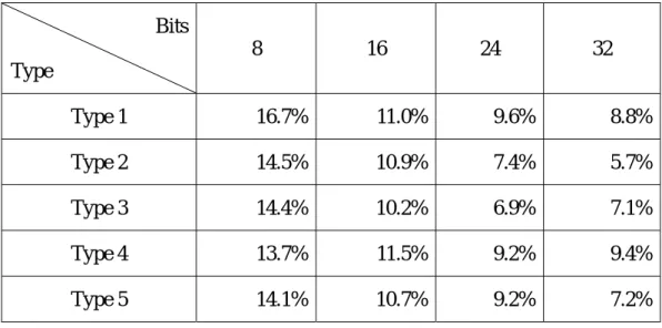
(26) Number of collisions of random bit-selection 1200000 1000000 Type Type Type Type Type. Times. 800000 600000 400000. 1 2 3 4 5. 200000 0 8. 16. 24. 32. Bits. Figure 5.1 Random bit-selection evaluations on sample 1. Bits 8. 16. 24. 32. Type 1. 334730. 219170. 191099. 176425. Type 2. 290827. 217678. 147322. 114019. Type 3. 287927. 203274. 137487. 141186. Type 4. 274241. 229052. 183860. 187722. Type 5. 282438. 213169. 184425. 143940. Type. Table 5.3 Random bit-selection evaluation on sample 2 (number of collisions). 19.

(27) Bits 8. 16. 24. 32. Type Type 1. 16.7%. 11.0%. 9.6%. 8.8%. Type 2. 14.5%. 10.9%. 7.4%. 5.7%. Type 3. 14.4%. 10.2%. 6.9%. 7.1%. Type 4. 13.7%. 11.5%. 9.2%. 9.4%. Type 5. 14.1%. 10.7%. 9.2%. 7.2%. Table 5.4 Random bit-selection evaluation on sample 2 (in collision ratios). Times. Number of collistions of random bit-selection 400000 350000 300000 250000 200000 150000 100000 50000 0. Type Type Type Type Type. 8. 16. 24. 32. Bits. Figure 5.2 Random bit-selection evaluations on sample 2. 20. 1 2 3 4 5.

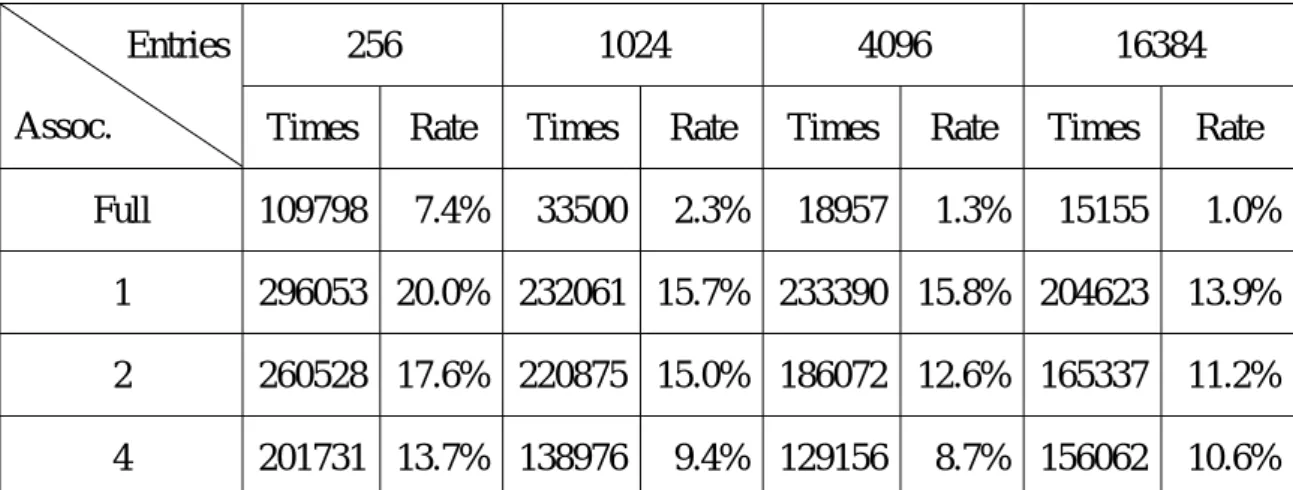
(28) 5.2 Simulation of IPv6 header caching We use the sample 2 for our experiment of IPv6 header caching. In order to simplify the experiment, packets belonging to “Other” category were omitted in the experiment. So the number of total packets is 1,476,591, instead of 2,000,000. We use random bit-selection with type 1 range, and hash function I in our simulations. The reason we use type 1 range is to complement the fields that hash function I ignores (prefixes of SA/DA, protocol).. 5.2.1 Miss ratios We evaluate the miss rates with different replacement policies, associativities, and cache sizes. Simulations of IPv6 header caching take much longer time than random bit-selection. Simulations of full associative cache memory take the longest time because the indices generated by random bit-selection are ignored, and almost lookups are performed with linear search. Experimental results are listed in Table 5.5 and 5.6. From the results, the miss rate is low even if the number of cache entries is 256 and associativity is one (direct-mapping). Increment of associativity or cache size decreases miss rate. Replacement policy does not affect the miss rate in direct-mapping, so the miss rates of different replacement policies are the same. Evaluation results of full associative with different replacement policies in Table 5.5 are omitted, because the number of total flows is below 18000, much less than 65536. Miss rate differences among the replacement policies are very small, so LRU is set to be the default replacement policy in latter evaluations. Evaluation results of full associativity in Table 5.6 are below 10%, most results. 21.

(29) are below 5%. Miss rates with associativity 4 and number of entries more than 1024 are also below 10%. So we can speedup the process of packet classification with a small cache memory.. LRU. Policy Assoc.. Times. LFU (limit=4). Rand. Rate. Times. Rate. Times. Rate. 1. 218643. 14.8%. 218643. 14.8%. 218643. 14.8%. 2. 131025. 8.8%. 158898. 10.8%. 164723. 11.2%. 4. 126149. 8.5%. 116147. 7.9%. 130646. 8.8%. Table 5.5 Miss rates with different replacement policies and associativities (# of entries=65536). Number of Miss times 250000. Times. 200000 LRU LFU (limit=4) Random. 150000 100000 50000 0 1. 2. 4. Associativity. Figure 5.3 Miss times with different replacement policies and associativities (# of entries=65536). 22.

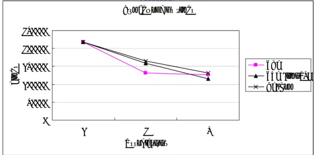
(30) 256. Entries Assoc.. 1024. 4096. 16384. Times. Rate. Times. Rate. Times. Rate. Times. Rate. 109798. 7.4%. 33500. 2.3%. 18957. 1.3%. 15155. 1.0%. 1. 296053 20.0% 232061 15.7% 233390 15.8% 204623. 13.9%. 2. 260528 17.6% 220875 15.0% 186072 12.6% 165337. 11.2%. 4. 201731 13.7% 138976. 10.6%. Full. 9.4% 129156. 8.7% 156062. Table 5.6 Miss Rates with different associativities and cache sizes (Replacement policy: LRU). Number of Miss times 350000 300000 Times. 250000. Full assoc. Direct mapping N=2 N=4. 200000 150000 100000 50000 0 256. 1024 4096 Number of entries. 16384. Figure 5.4 Miss Ratios with different associativities and cache sizes (Replacement policy: LRU). 23.

(31) Miss times 350000 300000. Times. 250000. 256 1024 4096 16384. 200000 150000 100000 50000 0 0. 1. 2. 4. Associativity. Figure 5.5 Miss ratios with different replacement policies and cache sizes (Replacement policy: LRU). 5.2.2 Misclassification ratios Misclassification means distinct flows are judged as the same one. So the misclassification rates should be as low as possible. We know that hash function I is independent of random bit-selection, but misclassification can be avoided completely because we compress the flow ID to 32 bit or less. To evaluate misclassification ratios, we place an extra field “flowID” in each cache entry to record original uncompressed flow ID. We check whether any two flows with same index and tag values are identical by the flowID field. Evaluation. results. show. that. increment. of. associativity. increases. misclassification rate because the length of index decreases with increase of associativity. So associativity should be chosen carefully when cache size is fixed. There has to be a trade-off between misclassification ratios and miss ratios. We found that the misclassified flows are very similar. Difference between the. 24.

(32) flows is only several bits. To avoid such misclassification, a complex hash functions for tag is needed. But hardware of complex hash functions is also complex, and not executed within only one step. Fortunately, misclassification ratios are almost below 5%. In direct-mapping, misclassification ratio is only 1.7%. So the probability of misclassification in practical packet processing is very little.. LRU. Policy Assoc.. Times. LFU Rate. Times. Rand Rate. Times. Rate. 1. 25082. 1.7%. 25082. 1.7%. 25082. 1.7%. 2. 58813. 4.0%. 65179. 4.4%. 54426. 3.7%. 4. 71486. 4.8%. 74138. 5.0%. 71673. 4.9%. Table 5.7 Misclassification ratios with different replacement policies and associativities (# of entries=65536). Times. Miss classification times 80000 70000 60000 50000 40000 30000 20000 10000 0. LRU LFU (limit=4) Random. 1. 2. 4. Associativity (bits). Figure 5.6 Misclassification ratios with different replacement policies and associativities (# of entries=65536). 25.

(33) 5.2.3 Hardware complexity Each cache entry contains a 32-bit Tag, an N-bit TS/Counter, an M-bit Result. There are (32+N+M)*X bits in a cache memory with X entries. Hardware cost increases with N and M.. 26.

(34) CHAPTER 6 CONCLUSIONS In this thesis, we proposed a cache architecture and hash functions to improve performance of packet classification for IPv6. Cache miss ratios in our evaluations are low even if cache size is small. Misclassification ratios are also low enough. High-speed packet processing is possible in future IPv6 environment and can be achieved with a cache memory at reasonable cost.. 27.

(35) CHAPTER 7 FUTURE WORK 7.1 IPv6 protocol chain problem In IPv6, options of IP are stored in extension headers instead of IP option fields in IPv4. The extensions are Hop-by-hop option (HBH), Source routing, Fragmentation, Authentication, Encrypted security payload (ESP), and Destination option. The IPv6 extension headers are inserted between IP header and ICMPv6/TCP/UDP header. They are linked with “Next header” fields in IP and extension headers. There are some packets with IPv6 option headers in our samples, but tcpdump cannot parse all the extensions with default buffer setting. To find the header of the layer-4 protocol for packet classification, routers must spend more time to trace the protocol chain. If the process of packet classification uses some speed-up skills such as pipeline, the extension headers will stall the pipeline and affect the throughput. Routers also must process the extension headers. It will be a big performance problem in practical IPv6 packet processing. It also will be a serious security problem to deal with packets with anomalous extension headers.. 7.2 Special layer-4 protocol processing There are some special layer-4 protocols other than ICMPv6, TCP, UDP in our samples. They are IP-in-IP (tunneling), and PIM. There may be some other special layer-4 protocols in real traffic. For IP-in-IP, there is another IP header encapsulated in. 28.

(36) the packet, and the header of layer-4 protocol is behind the encapsulated IP header. We must decide to process the encapsulated IP header or not. By the way, we must set the default action for all protocols not mentioned before.. 7.3 Use of flow label Flow label is a 24-bit field in IPv6 header to identify a flow effectively. Source host generates flow label randomly and must not reuse a flow label for a new flow while the existing flow is still alive. Unfortunately, there are only few packets set the flow label in our samples. Maybe we can use the flow label directly to speed up the process of packet classification if flow label is widely used in the future.. 29.

(37) REFERENCES [1] Pi-Chung Wang, Chia-Tai Chan, Shuo-Cheng Hu, “Performance Improvement of Packet Classification by Using Lookahead Caching,” IEICE Transactions on Communications, pp.377-379, 2004. [2] Pankaj Gupta and Nick McKeown, “Algorithms for Packet Classification,” IEEE Network vol.15, no.2, pp.24-32, Mar./Apr. 2001. [3] Sundar Iyer, Ramana Rao Kompella, and Ajit Shelat, “ClassiPI: An Architecture for Fast and Flexible Packet Classification,” IEEE Network vol.15, no.2, pp.33-41, Mar./Apr. 2001. [4] Masanori Uga, Kohei Shiomoto, “A novel ultra high-speed multi-layer table lookup method using TCAM for differentiated services in the Internet,” IEEE Workshop on High Performance Switching and Routing, 29-31 May 2001 [5] Kang Li, Chang, F., Berger, D., Wu-chang Feng, “Architectures for packet classification caching,” The 11th IEEE International Conference on Networks, Sept. 28-Oct. 1, 2003 [6] Gupta, P., McKeown, N., ”Classifying packets with hierarchical intelligent cuttings,” IEEE Micro, Volume: 20, Issue: 1, pp.34–41, Jan.-Feb. 2000.. 30.

(38)