數位訊號處理器中位址產生單元之位址位移配置最佳化

全文

(1)國立交通大學資訊工程系碩士論文. 數位訊號處理器中位址產生單元之位址位移配置最佳化. Address Offset Assignment Optimization for AGU in DSP Processor. 研究生：劉昆奇指導教授：單智君博士. 中華民國九十三年七月.

(2) 數位訊號處理器中位址產生單元之位址位移配置最佳化. Address Offset Assignment Optimization for AGU in DSP Processor Student：Kun-Chi Liu. 研究生：劉昆奇指導教授：單智君. 博士. Advisor：Dr. Jean, Jyh-Juin Shann. 國立交通大學資訊工程學系碩士論文 A Thesis Submitted to Department of Computer Science and Information Engineering College of Electrical Engineering and Computer Science National Chiao Tung University in Partial Fulfillment of the Requirements for the Degree of Master In Computer Science and Information Engineering July 2004 Hsinchu, Taiwan, Republic of China. 中華民國九十三年七月.

(3) 數位訊號處理器中位址產生單元之位址位移配置最佳化學生：劉昆奇. 指導教授：單智君博士國立交通大學資訊工程學系碩士班. 摘要近年來，嵌入式系統由嵌入式處理器、程式唯讀記憶體、隨機存取記憶體和特殊應用硬體組成單一電路的設計方式，在數位訊息處理的應用領域中逐漸增加。為了達到減少系統發展的花費以及上市的時間，在這類系統下開發程式的方式，也由組合語言轉變成使用高階的程式語言，如 C、C++和 Java。在本研究論文中，我們針對有限制的記憶體和具備位址產生器(AGUs)的嵌入式數位訊息處理器提出程式碼的最佳化技術。位址產生器提供間接定址模式(indirect addressing mode)，包括自動遞增(auto-increment)、自動遞減(auto-decrement)以及自動修改 (auto-modify)的動作，而有別於之前的研究重點僅在自動遞增和自動遞減的動作，我們提出 2 個方法：Pruning method 和基因演算法(Genetic Algorithm)，藉由同時利用上述的間接定址模式優勢，來減少位址計算所需的程式碼。我們的方法找出一組變數出在記憶體中的位址配置，使得需要用來明確計算變數位址的指令達到最少。根據實驗顯示，我們的方法較之前的研究，能更進一步改善 12%到 18%的位址計算指令程式碼。. i.

(4) Address Offset Assignment Optimization for AGU in DSP Processor Student：Kun-Chi Liu. Advisor：Jean, J.J Shann. Institute of Computer Science and Information Engineering National Chiao-Tung University. Abstract In recent years, embedded systems consist of embedded processor, program ROM, RAM and any application-specific hardware on a single circuit are becoming increasingly in application domains such as digital signal processing (DSP). In order to decrease development costs and time-to-market, programming manner on such systems is changed from assembly language to high-level languages such as C, C++ and Java. In this paper, we present code optimization techniques for embedded DSP processors which have limited on-chip ROM and address generation units (AGUs). AGUs provide indirect addressing modes with auto-increment, auto-decrement and auto-modify operations. We present two approaches：Pruning method and Genetic Algorithm that reduce address arithmetic code size by taking advantage of these addressing modes simultaneously while previous works only focus on auto-increment and auto-decrement operations. Our approaches find an address offset assignment for variables in RAM such that explicit instructions for address arithmetic are minimized. Experiment results show improvements of 12% to 18% over the previous works in address arithmetic code size.. ii.

(5) 誌謝. 本論文得以完成，首先要感謝單智君教授的辛勤指導與嚴格的督促，同時感謝實驗室的另一位指導老師鍾崇斌教授，多次提出批評與指正，使得論文更加嚴謹。在口試時，亦要感謝陳正教授與盧能彬教授所提出的寶貴意見，使得這篇論文更臻完整。此外，要感謝實驗室博士班馬詠程、謝萬雲、鄭哲聖與喬偉豪學長，對於我的研究提出問題並給予建議。還有，感謝實驗室的學長姐、同學以及學弟們的幫忙，不論是資料蒐集、程式技巧和寫作要點的討論等，都給予我莫大的助益，有你們的陪伴，更使我的研究生活更加充實與豐富。最後，我要感謝我的家人與好友長期地給予我支持與鼓勵，使我在兩年的碩士生涯中，能無後顧之憂地投入課業與研究之中。. — 謹將此論文獻給所有關心我、愛護我的師長及親朋好友. — 謝謝你們. 劉昆奇 2004/8/6 計算機系統實驗室. iii.

(6) Table of contents 摘要 ...................................................................................................... i Abstract ................................................................................................ ii 誌謝 .................................................................................................... iii List of Figures..................................................................................... vi List of Tables..................................................................................... viii Chapter 1 Introduction..........................................................................1 1.1 Research Motivations ...............................................................................2 1.2 Research Goal ...........................................................................................2 1.3 Design Approach.......................................................................................3 1.4 Organization of This Thesis......................................................................3. Chapter 2 Backgrounds.........................................................................4 2.1 Address Generation Units in DSPs ...........................................................4 2.2 The Genetic Algorithm .............................................................................9 2.3 Previous Researches Related to Address Offset Assignment Problem...14 2.3.1 Bartley’s Approach ......................................................................14 2.3.2 Other Address Offset Assignment algorithms..............................17 2.3.3 Summary......................................................................................20. Chapter 3 Proposed Approaches of Address Offset Assignment........21 3.1 Problem Modeling ..................................................................................22 3.2 Approach 1：Pruning Method for Address Offset Assignment .............26 3.3 Approach 2：Genetic Algorithm for Address Offset Assignment..........32 3.3.1 Chromosomal Representation and initialization..........................33 3.3.2 Crossover and Mutation Operators ..............................................34 3.3.3 Object Function............................................................................37 iv.

(7) 3.3.4 Stopping Criteria..........................................................................38 3.3.5 Parameters Setting in Genetic Algorithm ....................................38 3.4 Discussion...............................................................................................39. Chapter 4 Simulation Environment and Result ..................................41 4.1 Simulation Environment .........................................................................41 4.1.1 Simulation Flow...........................................................................41 4.1.2 OffsetStone Benchmarks .............................................................43 4.1.3. Address. Offset. Assignment. Approaches. in. Simulation. Environment.................................................................................................45 4.2 Simulation Results and Analyses............................................................46 4.2.1 Reduction of Code Size ...............................................................46 4.2.2 Influence of Modify Registers usage ...........................................50. Chapter 5 Conclusion and Future Work .............................................51 References...........................................................................................53. v.

(8) List of Figures Figure 2-1 Generic address generation unit (AGU) model for DSPs ............5 Figure 2-2 Example of address arithmetic with AGU ...................................8 Figure 2-3 General scheme of a Genetic Algorithm ....................................11 Figure 2-4 Access graph model and maximum weighted Hamiltonian path ..............................................................................................................16 Figure 2-5 Different address offset assignments and AGU operation sequences .............................................................................................17 Figure 2-6 Liao’s maximum weighted path cover heuristic algorithm........18 Figure 3-1 A Diagram of compilers for embedded systems ........................22 Figure 3-2 Example of distance count for different address assignment.....24 Figure 3-3 Code example from [12] ............................................................25 Figure 3-4 Different address assignment for Figure 3-3 example ...............25 Figure 3-5 An example of access graph for pruning....................................26 Figure 3-6 The solution of maximum weight path cover for Figure 3-5 .....27 Figure 3-7 An example of pruning for DFS.................................................29 Figure 3-8 Depth first search (DFS) for access graph .................................30 Figure 3-9 DFS with pruning for access graph............................................31 Figure 3-10 Example of genotypic representation.......................................33 Figure 3-11 Partial match crossover (PMX) operation................................35 Figure 3-12 Mutation operation ...................................................................37 Figure 4-1 Simulation Flow .........................................................................42 Figure 4-2 Cost reduction of approaches with 1AR and multiple MRs for small instances in benchmarks.............................................................48 Figure 4-3 Relative cost of approaches compared to OFU with 1AR for. vi.

(9) small instances in benchmarks.............................................................48 Figure 4-4 Cost reduction of approaches with 1AR and multiple MRs for all instances in benchmarks ......................................................................49 Figure 4-5 Relative cost of approaches compared to OFU with 1AR for all instances in benchmarks ......................................................................49 Figure 4-6 Relative cost compared to OFU with 1AR and multiple MRs for all instances in all benchmarks on average ..........................................50. vii.

(10) List of Tables Table 2-1 AGU operations and cost values....................................................6 Table 2-2 Comparison of address offset assignment researches..................20 Table 3-1 Comparison of time complexity for offset assignment algorithms with a single AR and multiple MRs.....................................................40 Table 4-1 Address arithmetic costs in benchmarks......................................47. viii.

(11) Chapter 1 Introduction In recently year, microprocessors such as microcontrollers and digital signal processors (DSPs) are increasingly used in embedded systems. System designer incorporate all the electronics ― microprocessor, program ROM and RAM, and application-specific circuit components ― into a single integrated circuit. Program code resides in on-chip ROM and program size translates directly into silicon area and cost. Program code size exceeds on-chip ROM size may lead to redesign of the whole system. It is an important goal of compiler for such architectures to generate compact code to meet the constraints of the limited on-chip ROM size. Many complimentary approaches have been employed to reduce code size including software-only techniques that rearrange data lay-out to reduce code size and instruction set support that allows generation of compact code [1]. Many embedded processors and DSPs (e.g., TI TMS320C25/50/80, Motorola DSP56k, ADSP-210x) provide address generation units (AGUs) that support indirect addressing mode with auto-increment, auto-decrement and auto-modify operations. AGUs allow for efficient sequential access of memory and subsume address arithmetic instructions. Subsuming the address arithmetic into auto-increment, auto-decrement and auto-modify modes improves both performance and code size [1,2]. The placement of variables in storage has a significant impact on the effectiveness of subsumption. Variables that are frequently accessed one after another are placed into neighboring storage locations during storage assignment. Then, the auto-increment and auto-decrement feature can be used and explicit address arithmetic instructions to set up the contents of the address register can be avoided. The problem of finding a storage layout which maximizes the use of auto-increment/decrement to reduce code size using a single address register (AR) is 1.

(12) called the Simple Offset Assignment (SOA) problem. When multiple address registers (ARs) are exploited, this problem is called General Offset Assignment (GOA) problem [2]. The storage offset assignment problem was first modeled as a maximum weighted Hamiltonian path cover (MWPC) problem by Bartley [3] and Liao et al. [1]. Further extensions have since been developed by many researchers. Leupers and Marwedel [2,4] improved Liao’s work by proposing a tie-breaking heuristic for SOA and a variable partitioning strategy for GOA to further reduce storage assignment cost.. 1.1 Research Motivations Experiment surveys indicate that about 20% - 30% (sometime even more than 50%) instructions of DSPs machine code used for address computations [5]. This is quite significant for DSPs with limited ROM size constraints. While previous SOA algorithms focus on auto-increment and auto-decrement operations and post-pass assign one modify register (MR) that stores frequently modify value for AR updates. The exploitation of auto-modify operations may lead to further reduce address arithmetic code.. 1.2 Research Goal In this thesis, we consider auto-increment, auto-decrement and auto-modify operations simultaneously to reduce address arithmetic code. Since the compiler determines the addresses of local scalar variables in the stack frame of a function. We find a data layout (address assignment) for these local scalar variables that AGUs with auto-increment, auto-decrement and auto-modify operations can be utilized to 2.

(13) subsume address arithmetic instructions and decrease code size. We also explore the influence of multiple modify registers used for auto-modify operation.. 1.3 Design Approach We provide two approaches：Pruning method and Genetic Algorithm (GA) to solve the address offset assignment problem that considers auto-increment, auto-decrement and auto-modify operations simultaneously. Pruning method is based on Bartley’s access graph [3] and traces all possible paths evaluated by our cost function in Chapter 3. Although pruning method can find optimal solution, the time complexity is still too high to solve large problem size. Then we apply Genetic Algorithm (GA) to solve our problem by modeling address assignment to chromosome representation and evolution via crossover and mutation operations. Experimental results show that our two approaches are effective.. 1.4 Organization of This Thesis This thesis is organized as follows. Chapter 2 introduces the address generation units feature and genetic algorithm which is an optimization technique. Then, we discuss previous relative researches on offset assignment problem. In Chapter 3, we describe our pruning method for finding data layout and apply genetic algorithm to our problem in detailed. The experimental environment and out simulation results are presented in Chapter 4. Finally, we summarize our conclusions and future work in Chapter 5.. 3.

(14) Chapter 2 Backgrounds In this chapter, we introduce the address generation units (AGUs) architecture in DSP processors. Then we introduce the Genetic Algorithm (GA) which is an optimization technique imitating natural evolution to achieve good solutions. Finally we discuss the previous researches related to address offset assignment problem to achieve code size reduction.. 2.1 Address Generation Units in DSPs Address generation units (AGUs) are the special architecture for memory address computation. DSP processors equipped with AGUs can perform indirect address computations in parallel to the execution of other machine instructions. The AGUs feature for indirect addressing are present in many DSP architectures (e.g., TI TMS320C25, Motorola DSP56k, ADSP-210x) and differ mainly in the following parameters [1,2]： . The number k of address registers (ARs). ARs store the effective addresses of variables in memory and can be updated by load and modify (i.e., adding or subtracting a constant) operations.. . The number m of modify registers (MRs). MRs can be loaded with constants and are generally used to store frequently required AR modify values.. 4.

(15) Figure 2-1 Generic address generation unit (AGU) model for DSPs. Further differences in the detailed AGU architectures of DSPs are whether MR values are interpreted as signed or unsigned numbers, and whether ARs and MRs are orthogonal, i.e., whether each MR can be used to modify each AR. We consider indirect addressing based on the genetic AGU model depicted in Figure 2-1. The AGU contains a file of k address registers and a file of m modify-registers. The indices for ARs and MRs are provided by two AGU inputs： The AR pointer (ARP) and the MR pointer (MRP). The third AGU input is an immediate value, originating from the instruction word, which can be used to load AR[ARP] or MR[MRP], or to immediately modify AR[ARP]. Further, AR[ARP] modification can also by adding or subtracting the contents of MR[MRP], or adding the value +1/–1.. 5.

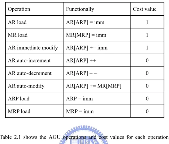
(16) Table 2-1 AGU operations and cost values Operation. Functionally. Cost value. AR load. AR[ARP] = imm. 1. MR load. MR[MRP] = imm. 1. AR immediate modify. AR[ARP] += imm. 1. AR auto-increment. AR[ARP] ++. 0. AR auto-decrement. AR[ARP] – –. 0. AR auto-modify. AR[ARP] += MR[MRP]. 0. ARP load. ARP = imm. 0. MRP load. MRP = imm. 0. Table 2.1 shows the AGU operations and cost values for each operation. The functionalities are given in C-like notation, where “imm” denotes an immediate value. Further, immediate value occupies a large portion of the total instruction word-length, so that these operations usually inhibit execution of other machine instructions in parallel. Like all other register transfer (RT) patterns, we assume AGU operations to be executed in a single machine cycle, so that the results are valid in the following cycle. “AR load”, “MR load”, and “immediate modify”, which involve immediate value in the instruction word. These operations cannot be performed in parallel to other operations, but introduce an extra machine instruction. Therefore, we assign the cost value 1 to these operations. On the other hand, “auto-increment”, “auto-decrement”, and “auto-modify” only utilize AGU resource and can be regarded as zero-cost operations. These operations can be executed without any overhead in code size or speed. The same hold for “ARP load” and “MRP load”： These require. 6.

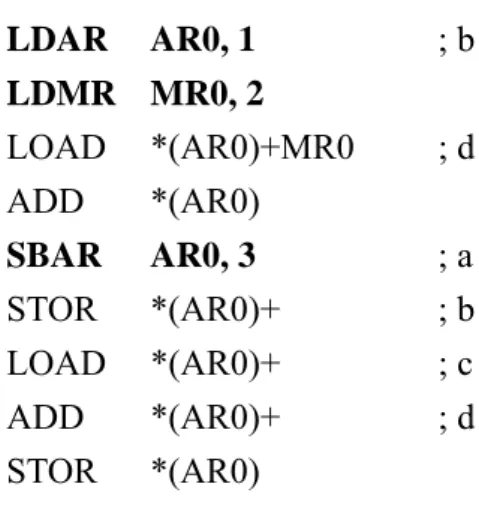
(17) only “short” immediate values (of length 2 to 3), which are (in direct form) instruction word fields, or (in indirect form) originate from registers which can be loaded in parallel (e.g., TMS320C2x). In indirect form, the required ARP contents must be prepared one machine cycle earlier than in direct form, but this has no impact on the cost metric [2].. Example To simplify the exposition of address offset assignment, we use a simple processor model that reflects the indirect addressing arithmetic of most DSPs. The model is an accumulator-based machine where, for each instruction, one operand resides in the accumulator and another operand resides in the memory. The operand involves memory is referenced through one of the address registers (AR0, AR1 …). ARi can point to the desired position by adding or subtracting an immediate value, using the instructions “ADAR” and “SBAR”. Also, we use the instructions “LDAR” and “LDMR” to load ARi and MRi. We use *(ARi), *(ARi)+, *(ARi)-, *(ARi)+MRi to denote indirect addressing through ARi, indirect addressing with post-increment, indirect addressing with post-decrement and indirect addressing with post-modify, respectively. Consider the C code sequence shown in Figure 2-2(a). Assume that the address offset assignment to the various variables is as shown in Figure 2-2 2-2(b). The assembly code for the C program is shown in Figure 2-2(c). In the assembly code, the comment after an instruction indicates which variable AR0 point to after the instruction is executed. The instruction SBAR and ADAR are used to change AR0 to point to the frame location accessed in the next instruction.. 7.

(18) a=b+d; d=b+c;. LDAR. LDMR MR0, 2 LOAD *(AR0)+MR0 ADD *(AR0). (a) Code sequence. AR0. 0. a. 1. b. 2. c. 3. d. AR0, 1. SBAR STOR LOAD ADD STOR. AR0, 3 *(AR0)+ *(AR0)+ *(AR0)+ *(AR0). ;b ;d ;a ;b ;c ;d. (c) Assembly code. (b) Offset assignment. Figure 2-2 Example of address arithmetic with AGU Assume that AR0 initially points to the position 1 of the frame, i.e., variable b and MR0 is initialized by a constant 2. The value of the variable b is loaded in the accumulator, and AR0 is modified by the value of MR0 in the first “LOAD” instruction. In the fourth instruction “ADD”, the values in b and d are summed and stored in the accumulator. Next, the contents of the accumulator must be stored in the location corresponding to variable a, but AR0 point to d. Therefore, we have to subtract 3 from the content of AR0 using an explicit instruction “SBAR AR0, 3”. Then, the instruction “STOR” is used to store the contents of accumulator to the location of a; futher, AR0 is incremented and points to the location of b. When the assembly instructions corresponding to “d = b + c” are to be executed, variables access order of variables is b, c, then d. We can see that the locations of these variables are continuous in Figure 2-2(b). So, these address arithmetic operations can be subsumed in “LOAD”, “ADD” or “STOR” instructions. The objective of the solution to the address offset assignment is to find the minimal address pointer arithmetic instructions required using proper placement of variables in memory.. 8.

(19) 2.2 The Genetic Algorithm Genetic Algorithms belong to a certain group of heuristic problem solving techniques based on the principles of natural evolution. To this group of Evolutionary Algorithms belong also Evolutionary Programming, Evolution Strategies, and Genetic Programming. They share a common conceptual base of simulating the evolution of individual structures via processes of selection, mutation, and reproduction. The processes depend on the perceived performance of the individual structures as defined by an environment [6, 7]. More precisely, Evolutionary Algorithms maintain a population of structures, that evolve according to rules of selection and other operators, that are referred to as search operators, (or genetic operators), such as recombination and mutation. Each individual in the population receives a measure of it’s fitness in the environment. Reproduction focuses attention on high fitness individuals, thus exploiting the available fitness information. Recombination and mutation perturb those individuals, providing general heuristics for exploration. Although simplistic from a biologist’s viewpoint, these algorithms are sufficiently complex to provide robust and powerful adaptive search mechanisms [6, 7]. Genetic Algorithms were devised by John Holland. The Genetic Algorithm is a model of machine learning which derives its behavior from a metaphor of some of the mechanisms of evolution in nature. This is done by the creation of a population of individuals of individuals represented by chromosomes, in essence a set of character strings that are analogous to the base-4 chromosomes that we see in our own DNA. The individuals in the population then go through a process of simulated evolution. Implementations typically use fixed-length character strings to represent their genetic information, together with a population of individuals which undergo crossover and. 9.

(20) mutation in order to find interesting regions of the search space [6, 7].. Standard Formulation Genetic Algorithms are working on a population of individuals that undergo an evolution. This evolution is caused by manipulating the chromosomes of the individuals of the current generation by mutation and crossover. The Genetic Algorithm selects those offspring individuals for the next generation that perform best in a defined environment (that possess the highest fitness). That means that only the fittest survive and the average fitness of the population will increase. For that reason the population adapts itself optimally to the environment after a certain number of generations. If the fitness of the individuals is chosen according to the objective function f and the genes of the chromosomes are seen as the genome representation of optimization variables x1, x2, …xm then a Genetic Algorithm can be used to solve the multidimensional optimization problem [6]： f (x1, x2, …xm) => optimum Figure 2-3 shows the general scheme of Genetic Algorithm. At the beginning a population of nP individuals is created and initialized. The initialized is usually done by filling the chromosomes of the individuals with random values. The initial generation will then be evaluated. The fitness of the particular individuals is calculated and the population is ordered with respect to fitness. To evaluate the fitness of the individuals the phenotypic representation of the individual must be derived from the genotypic one. That means in context of the considered optimization problem the optimization variable x1, x2 …xm must be calculated from the chromosomes which are typically fixed-length bit string.. 10.

(21) Initialize. nP Select parents Apply crossover. Best parents. nE. nP Apply mutation. nE + nP Evaluate fitness Delete last nP. Stop?. Finish. Figure 2-3 General scheme of a Genetic Algorithm. At the beginning of each cycle the current generation (parent generation) will reproduce itself. This is performed in two steps [6]： First, the nE best of the current generation will be copied into the next generation. This is also known as elitist approach because it can lead to the formation of elite in the population. Elitist individuals can survive a long time in the population. Second, two of individuals in the parent generation exchange parts of their chromosomes to create two children. This process is called crossover and occurs with a probability px. Typical values px are in the range between 0.4 and 0.8. So nP /2 pairs 11.

(22) of parents will produce nP children. After reproduction the new population has size nE + nP. To select pairs of parents the following selection techniques are considered： . Random parent selection (RS)： The parent is chosen randomly from the parent generation. All individuals have the same chance to become a parent.. . Tournament parent selection (TS)： Two individuals are chosen randomly. As parent is used that individual with the higher fitness. This guarantees that fitter individuals become more often parents than others.. . Roulette wheel parent selection (RWS)： The parent is chosen randomly, but its chance to be chosen as parent is proportional to its fitness. This is done as follows： Calculate the total fitness as sum of the fitness values of all the population members. Generate n, a random number between 0 and total fitness. Select the first population member whose fitness, added to the fitness of the preceding population members, is greater than or equal to n. Note, that the fitness values must be nonnegative numbers. This selection technique also guarantees that fitter individuals become more often parents than others.. After the parent selection the actual crossover can take place. During the crossover the parents exchange parts of their chromosomes. This is done in order to be able to combine good chromosome parts in the offspring, to create better chromosomes from good ones. There exit different ways of how parents can exchange chromosome parts. Which crossover operator performs best depends on the problem at hand. The following three variants can be applied to a variety of problems [6,7]： . Single point crossover (SPX) ： A random position is chosen in the chromosome. The chromosome parts after this position are exchanged.. . Dual point crossover (DPX)： Two random positions are chosen in the chromosome. The chromosome parts between these positions are 12.

(23) exchanged. . Uniform crossover (UX)： For each bit position there is a random decision which parents contributes its bit value to which child. The exchange of chromosome parts is controlled by a random template.. After reproduction mutation are applied to the population. This is done by flipping bits in the chromosomes of the individuals. The bit flipping occurs with a certain probability pM. A typical value for pM is 0.01. The purpose of the application of mutations is to introduce a certain amount of diversity into the population. Then, the individual’s fitness is calculated according to the objective function f. The population is ordered with respect to fitness and the last nE individuals are deleted from the population. This is the second point in the algorithm where a selection according to fitness takes place. If as parent selection technique random selection is used then it is necessary to set the number of elitist individuals nE greater than 0. Otherwise no directed development over the generations can occur. On the other hand, if random parent selection is not used, then nE can be set to 0 and the time consuming ordering of the population can be avoided. Until now, a new generation of nP individuals was generated and process of reproduction, mutation, and selection can start again. If all parameter values of the algorithm are set reasonably and crossover operator, mutation operator and representation are chosen appropriately then the Genetic Algorithm will converge after a certain number of generations to the solution of the considered optimization problem.. 13.

(24) 2.3 Previous Researches Related to Address Offset Assignment Problem In the following subsection, we describe access graph model for Offset Assignment problem first proposed by Bartley. Then we introduce previous researches about Offset Assignment problem. Finally we compare these algorithms with our research in last subsection.. 2.3.1 Bartley’s Approach Bartley was the first to address the simple offset assignment (SOA) problem that considered a single address register (AR). He proposed the access graph model for SOA problem and presented an approach based on finding a maximum weighted Hamiltonian path [2, 8].. Definition 2-1 Given a local scalar variable set V = {v1 ,..., v n } and a variable access sequence S = {s1 ,..., sm } of a function with ∀i ∈ [1, m] : si ∈ V , the access graph is an undirected, complete, and edge-weighted graph G = (V , E , w). with E = {{vi , v j } | vi , v j ∈ V } . The function w : E → Ν 0 assigns a weight to each. edge e = {vi , v j } that denotes the number of access transitions between vi and vj in S, i.e., the number of subsequence of S of the form (vi, vj) or (vj, vi). Definition 2-2 For an access sequence S on variable set V, an address assignment. is a mapping π : V → {0,..., | V | −1} , which assignment all variables in V to a unique location within a contiguous address space of size |V|. Due to the symmetry of auto-increment and auto-decrement, the ordering of v and w is irrelevant here. Likewise, self-edges of the form {vi, vj} can be neglected.. 14.

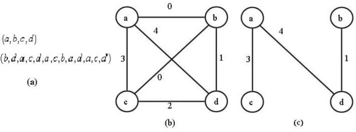
(25) Definition 2-3 The distance δ π ( vi , v j ) of two variables vi , v j ∈ V with respect. to π is π ( vi ) − π ( v j ) . Definition 2-4 Let G = (V , E , w) be the access graph for S. The cost of an. address. assignment. π. is. defined. as. cos t (π ) = 1 +. ∑ w(e). with. ^. e ={vi , v j }∈E. ^. E = {{vi , v j } ∈ E | δ π (vi , v j ) > 1} .. Simple Offset Assignment is the problem of computing a minimum cost address. assignment for an access graph G in presence of a single address register. In Figure 2-4(a)-(b), we see an example of access graph model G = (V , E , w) for V = {a, b, c, d } and S = (b, d , a, c, d , a, c, b, a, d , a, c, d ) . Any access transition (vi, vj) in S can be implemented by auto-increment, if and only if vi and vj are assigned neighboring stack locations. In order to maximize the use of auto-increment addressing, obviously those variable pairs {vi, vj} should be neighbors in the stack frame, whose edge weight w({vi, vj}) in G is high, since this will save many extra instructions for address computation. Figure 2-4(c) shows the maximum weighted Hamiltonian path cover (MWPC) P in G, i.e. the path touching each node once with the maximum edge weight sum. The memory layout is derived from P by assigning those node pairs to adjacent memory locations, which are also neighboring in P (i.e., c-a-d-b or b-d-a-c in Figure 2-4(c)) [2, 8].. 15.

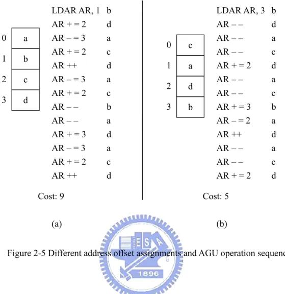
(26) Figure 2-4 Access graph model and maximum weighted Hamiltonian path. Suppose, address space reserved for V is A = {0, 1, 2, 3} and one AR is available to compute the address according to the sequence S. Consider an address assignment where V is mapped to A in lexicographic order (as shown in Figure 2-5(a)). First, AR needs to be loaded with the address 1, so as to point to the first element b of S. Then, AR is modified by +2 to access d which is mapped to address 3, and so forth. The complete AGU operation sequence for S is given in Figure 2-5(a). Only 4 out of 13 AGU operations in the sequence are auto-increment/decrement operations, so that a cost of 9 extra instructions for address computation is incurred. However, one can find a better address offset assignment by MWPC, which leads to only five extra instructions, due to a better utilization of zero-cost operations (as shown in Figure 2-5(b)).. 16.

(27) 0. a. 1. b. 2. c. 3. d. LDAR AR, 1 AR + = 2 AR – = 3 AR + = 2 AR ++ AR – = 3 AR + = 2 AR – – AR – – AR + = 3 AR – = 3 AR + = 2 AR ++. b d a c d a c b a d a c d. 0. c. 1. a. 2. d. 3. b. LDAR AR, 3 AR – – AR – – AR – – AR + = 2 AR – – AR – – AR + = 3 AR – = 2 AR ++ AR – – AR – – AR + = 2. Cost: 9. Cost: 5. (a). (b). b d a c d a c b a d a c d. Figure 2-5 Different address offset assignments and AGU operation sequences. 2.3.2 Other Address Offset Assignment algorithms Bartley’s access graph model for the SOA problem forms the baseline for most SOA algorithms. The cost of an SOA problem P is defined as the sum of the weights of G’s edges not covered by P. This corresponds to the number of extra address computation instructions to be inserted into the machine code. Because the classical Hamiltonian path problem that computing P is an NP-complete problem. Hence, many heuristic algorithms had been proposed to solve SOA problem [2]. Bartley proposed a greedy heuristic for finding path P. His algorithm iteratively picks an edge e of highest weight w(e) in G and checks whether inclusion of e into a partial path P would still allow for a valid solution. This is iterated until a complete path with V − 1 edges has been selected [2]. 17.

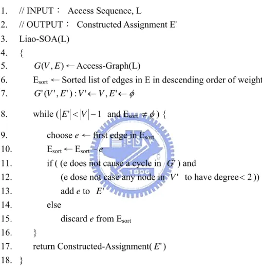
(28) Liao proposed a more efficient implementation of Bartley’s SOA algorithm, by temporarily neglecting edges of zero weight (which are frequent in realistic access graphs) and using an efficient Union/Find data structure for checking for cycles. Besides the implementation issues, Liao’s algorithms produces the same results as Bartley’s [1,2]. 1. 2.. // INPUT： Access Sequence, L // OUTPUT： Constructed Assignment E'. 3. 4. 5.. Liao-SOA(L) { G (V , E ) ← Access-Graph(L). 6. 7.. Esort ← Sorted list of edges in E in descending order of weight G ' (V ' , E ' ) : V ' ← V , E ' ← φ. 8.. while ( E ' < V − 1 and Esort ≠ φ ) {. 9. 10.. choose e ← first edge in Esort Esort ← Esort – e. 11. 12.. if ( (e does not cause a cycle in G ' ) and (e dose not case any node in V ' to have degree < 2 )). 13. 14. 15. 16. 17. 18. }. add e to E ' else discard e from Esort } return Constructed-Assignment( E ' ). Figure 2-6 Liao’s maximum weighted path cover heuristic algorithm. Leuper and Marwedel proposed a tie-break heuristic for choosing among same-weighted edges extended from Liao’s heuristic algorithm. These same same-weight edges are very common in access graphs, and the solution quality may critically depend on the order in which edges are investigated during path construction. 18.

(29) An experiment evaluation for a set of random SOA problem instances indicated that the tie-break heuristic on average gives a slight improvement over Liao’s heuristic [9]. Atri et al. proposed an incremental SOA algorithm. It starts with an initial SOA solution, constructed by some heuristic, and performs an iterative improvement by a local exchange of access graph edges selected for the maximum weighted Hamiltonian path. An experiment comparison to Liao’s heuristic for a set of random SOA instances indicated that the initial solution can be improved in 3-8% of the cases considered, where the average improvement is about 5% [10,11]. The general offset assignment (GOA) problem is the generalization of SOA towards an arbitrary number m of ARs. Lioa pointed out that GOA can be solved by appropriately partitioning V into m subsets, thereby reducing GOA to m separate SOA problems. Leupers and David proposed a genetic algorithm to solve GOA problem and experimental evaluation indicated a significant improvement than previous GOA researches [2].. 19.

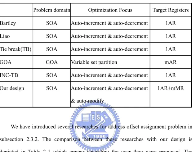
(30) 2.3.3 Summary. Table 2-2 Comparison of address offset assignment researches Problem domain. Optimization Focus. Target Registers. Bartley. SOA. Auto-increment & auto-decrement. 1AR. Liao. SOA. Auto-increment & auto-decrement. 1AR. Tie break(TB). SOA. Auto-increment & auto-decrement. 1AR. GOA. GOA. Variable set partition. mAR. INC-TB. SOA. Auto-increment & auto-decrement. 1AR. Our design. SOA. Auto-increment & auto-decrement. 1AR+mMR. & auto-modify. We have introduced several researches for address offset assignment problem in subsection 2.3.2. The comparison between these researches with our design is depicted in Table 2-1 which appear according the year they were proposed. The problem domain is classified according to how many address registers used. Because our design considers single address register with multiple modify registers, we categorize our design to SOA problem. The third column specifies the optimization focus of researches. While previous SOA researches focus on auto-increment and auto-decrement operations and post-pass assign MR. Our design consider auto-increment, auto-decrement and auto-modify operations simultaneously and exploit multiple MRs to further reduce address computation code. The last column is the target registers that researches focus on.. 20.

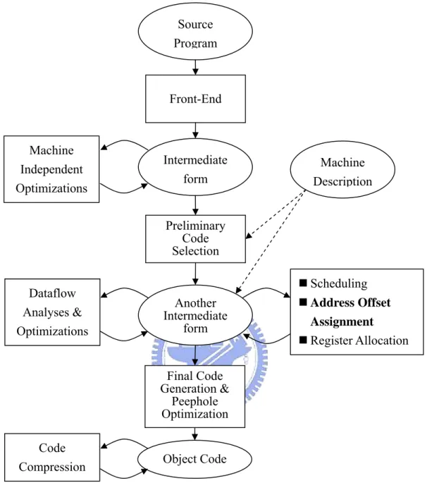
(31) Chapter 3 Proposed Approaches of Address Offset Assignment The address offset assignment optimization is incorporated into compilers for embedded systems. The diagram illustrates the stages of the compiler is shown in Figure 3-1. Source program is translated into intermediate form by one Front-End that includes error checking, lexical, syntax, and semantic analysis. Machine-independent optimizations such as constant folding, dead code elimination…, etc. The intermediate form is then translated into another intermediate form according to the machine description. Instruction scheduling, address offset assignment, and register allocation are performed on this intermediate form, along with machine-specific dataflow analysis and related optimizations. Object code is generated from the final code generation and peephole optimization. Code compression maximizes parallelism of object code to increase the code density [1, 2]. In this chapter, we present our design for address offset assignment. First, we model our address offset assignment problem that considers one address register and multiple modify registers simultaneously. Then we proposed two approaches for address offset assignment problem. In section 3.2, we present a pruning method combined with depth-first search (DFS) to find optimal solution for small instances. In section 3.3, we model our problem to apply Genetic Algorithm to solve this problem. Finally, we discuss these two approaches with previous researches about time complexity and usage in compiler.. 21.

(32) Source Program. Front-End. Machine Independent Optimizations. Intermediate form. Machine Description. Preliminary Code Selection Scheduling. Dataflow Analyses & Optimizations. Another Intermediate form. Address Offset Assignment Register Allocation. Final Code Generation & Peephole Optimization Code Compression. Object Code. Figure 3-1 A Diagram of compilers for embedded systems. 3.1 Problem Modeling In our design, we consider the usage of multiple modify registers that store frequently modify values for AR updates. So we define the term “count” that represents the count of distance after address assignment of variables. Then we define the cost function via the “count”. Definition 3-1 The distance count count(d) is the sum of w(e) where e = {vi, vj} 22.

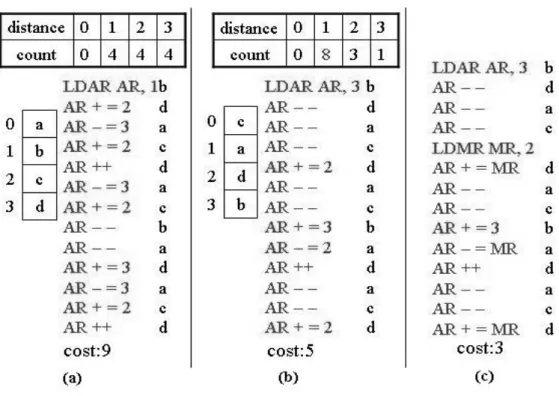
(33) and δ π ( vi , v j ) = d ,0 ≤ d ≤ V − 1 . Definition 3-2 Consider the usage of a single address register and m modify. registers. The cost of an address assignment π is defined as cost( π ) = 1 + n +. V −1. ∑ k =2. count (k) − ∑ (the first n maximum count (d)). , where n is the number of the first n maximum count(d) that count ( d ) > 1 , 0 ≤ n ≤ m , 2 ≤ d ≤ V − 1 . Because we consider the best usage of AGUs, not all the. m modify registers are used for each instance. To initialize an address register or a modify register need the cost 1. So the cost to initialize a single address register and n modify registers is 1+ n. For the purpose of illusion, we give two examples to see the influence when address assignment is assigned for modify registers. We first see the distance count for Figure 2-5 in Figure 3-2. The modify values in Figure 3-2(a) and Figure 3-2(b) are the distances of variables after address assignment. We calculate the number for each distance in code sequence and establish distance count table. Figure 3-2(b) is the result of maximum weighted Hamiltonian path cover and maximizes count of distance 1 that can be subsumed by auto-increment or auto-decrement operations. The count 3 of distance 2 is the maximal count of all distances larger than 1. Consider one modify register is used, distance 2 is assigned to modify register and the cost is decrease to 3 in Figure 3-2(c). Let us see a more complex example from [12] in Figure 3-3. The variable set and access sequence are extracted from the C code, and the access graph is constructed. The path that edges are bold in access graph is the solution of tie-break algorithm. We observe different address assignments ： TB solution, Address assignment 1 and Address assignment 2 in Figure 3-4. TB solution is the result from Figure 3-3, 23.

(34) Figure 3-2 Example of distance count for different address assignment. Address assignment 1 and Address assignment 2 are the optimal solutions for 1AR with 1 MR and 1AR with 2MRs respectively. For each address assignment, its distance count table is also shown in Figure 3-4. We know that distance 1 can be subsumed by auto-increment or auto-decrement operations and distance larger than 1 can be subsumed by auto-modify operation via assigning distances to modify registers. We can see that when only one AR is considered, the minimal cost is 13 in Figure 3-4(a) (i.e. Tie-Break solution). But when MR is considered, the minimal cost is 8 with 1AR and 1MR in Figure 3-4(b) and the minimal cost is 5 with 1AR and 2MRs in Figure 3-4(c). Therefore, the good address assignment for auto-increment and auto-modify operations is not necessarily good when auto-modify operation is considered. Problem Definition. Our design for address offset assignment problem is to compute a minimum cost. 24.

(35) of address assignment for an access graph G in presence of a single address register and multiple modify registers.. Figure 3-3 Code example from [12]. Figure 3-4 Different address assignment for Figure 3-3 example 25.

(36) 3.2 Approach 1：Pruning Method for Address Offset Assignment In this section, we describe a pruning method for the address offset assignment problem in presence a single address assignment and m modify registers. We trace access graph and decrease search time by pruning some paths that are not possible to be optimal solution. Given a variable set V and a variable access sequence S of a function, the Bartley’s access graph is constructed in Figure 3-5 and the maximum weight path cover is shown in Figure 3-6(a). From the maximum weight path cover, the address assignment is in Figure 3-6(b). Consider 1AR and 1MR for this example, we get the distance count in Figure 3-6(c) derived from the address assignment in Figure 3-6(b). The distance is 1 can be subsumed by auto-increment or auto-decrement operations, and the distance is 3 can be subsumed by auto-modify operation via assigning 3 to MR. Then we calculate the cost by the cost function in definition 3.5. So the total cost is 6 in Figure 3-6(d) is the cost of initial 1AR and 1MR, and distance count that can not be subsumed by auto-increment, auto-decrement, and auto-modify operations (count of distance 2 or 4).. Figure 3-5 An example of access graph for pruning 26.

(37) Figure 3-6 The solution of maximum weight path cover for Figure 3-5. Then, we explore the access graph in Figure 3-5 using depth-first search (DFS) that each vertex in access graph can be the original source and take the cost in Figure 3-6(d) as the cost bound to pruning some search path that cost is larger than cost bound. The strategy followed by depth-first search is, as its name implies, to search “deeper” in the graph whenever possible. In depth-first search, edges are explored out of the most recently discovered vertex u that still has unexplored edges leaving it. When all of u’s edges have been explored, the search “backtracks” to explore edges leaving the vertex from which u was discovered. This process continues until we have discovered all the vertices that are reachable from the original source vertex. If any undiscovered vertices remain, then one of them is selected as a new source and the search is repeated from that source. This entire process is repeated until all vertices are discovered. Next, we give an example to see the pruning operation. Consider the example in Figure 3-7(a). The DFS start from node “a” and explore to “c” currently (edges in bold). The current address assignment is shown in Figure. 27.

(38) 3-7(b) that “a” is assigned the address “0”, “b” is “1”, and “c” is “2”. The current distance count is shown in Figure 3-7(c) that the count of distance 1 is 2 ( w( a, b) + w(b, c ) ) and the count of distance 2 is 3 ( w( a, c ) ). Because the current distances are only 1 and 2, which can be subsumed by auto-increment, auto-decrement and auto-modify operation. So the current cost 2 is the cost of initializing 1AR and 1MR. Now there are two uncovered nodes “d” and “e” that are adjacent to node “c”. First, we choose node “d” as shown in Figure 3-7(e), and the current address assignment and distance count are shown in Figure 3-7(f) and Figure 3-7(g). And the current cost 7 in Figure 3-7(h) is cost of 1AR and 1MR initialization and distance count that can not be subsumed by auto-increment, auto-decrement and auto-modify operations (count of distance 3). Here, we find that the current cost 7 is larger than cost bound 6, so we stop search deeper from node “d” in current path and backtrack to node “c”. Therefore, we choose another node “e” that is adjacent to node “c” in Figure 3-7(a). The results of this choice are shown in Figure 3-7(i) to Figure 3-7(l). The current cost is not larger than cost bound, so we this search can be continue and will not be pruned. Via our pruning method, we can search all possible paths to find the optimal solution and save some search time. The algorithms of our pruning method are in Figure 3-8 and Figure 3-9. We will discuss our pruning method with previous searches and our genetic algorithm about the time complexity and effect in later section and chapter.. 28.

(39) Figure 3-7 An example of pruning for DFS. 29.

(40) Consider the algorithm in Figure 3-8. This algorithm takes an access sequence “L” which extracted from high level code as input, and produces an address offset assignment as output. In line 3, access graph G (V , E , w) is produced from the access sequence “L”. Line 4 produces an address offset assignment π 1 by Liao’s SOA heuristic algorithm mentioned in Chap 2. We set the cost_bound via the cost function in definition 3.5 that takes π 1 as its input. Then we start to explore the access graph G (V , E , w) using depth-first search (DFS) that each vertex in G can be the original source. The DFS-VISIT implements the DFS procedure with pruning.. 1 2. // INPUT： Access Sequence, L // OUTPUT： Constructed Assignment to minimize the cost. 3. function in definition 3.5. G (V , E , w) ← Access-Graph(L). π 1 ← Liao-SOA(L). 4 5 6. cost_bound ← count_cost( π 1 ) // Use Depth First Search (DFS) to trace G(V , E, w). 7. for each vertex u ∈ V {. if (u is not explored) 8 9 DFS-VISIT(u) 10 } 11 // When finished, we get the optimal solution π. Figure 3-8 Depth first search (DFS) for access graph. Consider the procedure DFS-VISIT in Figure 3-9. In each call DFS-VISIT(u), vertex u is checked if it can be added to tmp _ π that record the current unfinished address offset assignment. Lines 2-3 add u to tmp _ π in order and set u is explored. Line 4-5 check compute the cost of tmp _ π and check cost. When cost ≥ cost_bound, we prune the following process of tmp _ π and leave DFS-VISIT(u). Otherwise, if 30.

(41) 1 2. DFS-VISIT(u) { Add u to tmp _ π in order. 3 4. set u is explored cost ← count_cost( tmp _ π ). 5. if (cost ≤ cost_bound) {. 6. if ( tmp _ π = V ) {. 7. π ← tmp _ π. 8 9 10 11 12 13 14 15 16. cost_bound ← cost } else { for each v adjacent to u { if (v is unexplored) DFS-VISIT(v) } } } delete u in tmp _ π. 17 18 }. set u is unexplored. Figure 3-9 DFS with pruning for access graph. cost less than cost_bound, we further check the size of current tmp _ π in line 6. If the size of current tmp _ π is equal the size of variable set, this means that one solution is found. We record the current best solution in π and reset cost_bound from this solution in lines 7-8. If all variable are not covered, line 11 examines each vertex v adjacent to u and recursively visit v. We say that edge (u, v) is explored by the depth-first search. Finally, after every edge leaving u has been explored, lines 16-17 delete u in tmp _ π and set u is unexplored. This causes the next search from the predecessor of u. When all vertex u is explored, the algorithm is stopped and we get the optimal path (i.e., the optimal address offset assignment).. 31.

(42) 3.3 Approach 2：Genetic Algorithm for Address Offset Assignment The Genetic Algorithm (GA) is an optimization technique that imitates natural evolution to achieve good solutions. GA is particularly well-suited for nonlinear optimization problems, since it can skip local extreme in the objective function and in general come close to optimal solutions. We choose GA for solving address offset assignment problem in presence of a single address register and multiple modify registers mainly due to three reasons：First, GA is more robust than heuristic algorithms. If enough computation time is invested, then a GA most likely approximates a global optimum, while heuristics in many cases are trapped in a local optimum. Since very high compilation speed is not important for DSP compilers, GA is more promising than heuristics, whenever a reasonable amount of time is not exceeded. Second, since address offset assignment mainly demands for computing a good permutation of variables w.r.t. simple cost functions, address offset assignment has a straightforward encoding as a GA. Third, although the pruning method mentioned in section 3.2 can find the optimal solution, it can’t deal with large variable set. The complexity for large instance is too high for pruning method to find the optimal solution in a reasonable time. The influence of the size of variable set for GA is not critical. In this section, we present our problem the address offset assignment problem in presence of a single address register and multiple modify registers in the form of a GA. We describe the chromosomal representation for our solution, crossover and mutation operators for chromosome, objection function to judge chromosome’s fitness, the stop criteria of GA process and other parameters for GA.. 32.

(43) 3.3.1 Chromosomal Representation and initialization In order to apply a Genetic Algorithm to the address assignment problem an appropriate genotypic representation must be chosen. An obvious possibility is to use chromosomes with a number of genes equal to the number of variables where each gene represents a variable that is assigned to a memory location. This is an order-based representation that represents any solution to our problem. Assume we have a variable set V = {a, b, c, d, e, f, g}, Figure 3-10 shows two examples of our genotypic representation. Chromosome 1 and chromosome 2 represent two possible solutions to our problem. In chromosome 1, the order-based representation means an address offset assignment for the variable set V (d → 0, a → 1, b → 2 … and so on.) and the same in chromosome 2.. Chromosome. d a. b c. f. g e. Figure 3-10 Example of genotypic representation. In our design for GA, we initialize the individuals with such chromosomes in population. We start with Liao’s and Tie-Break’s SOA solutions which are discussed in Chap 2. We choose the minimum cost by applying our cost function in Definition 3-2 from these two solutions. Then we translate the solution to the form of genotypic. representation and use it to initialize the first chromosome of individual. This chromosome is the primordial genetic material from which all solutions will evolve.. 33.

(44) 3.3.2 Crossover and Mutation Operators A special property of our address offset problem and other similar combinational problems is that the genes cannot be treated independent of each other. That’s because each variable is allocated to one memory location and therefore, each variable may only appear once in the chromosome. Standard crossover and mutation operators which don’t take into account these dependencies will produce partly illegal offspring. One approach of dealing with that fact would be to use a standard Genetic Algorithm and to assign small or zero fitness to illegal ones. This could work in case when the number of illegal individuals is small in comparison to the legal ones. This cannot be expected for our problem. That’s why reproduction operators must be used that only yield offspring with legal genotypic representations. In the following, we describe our reproduction operators：Crossover and mutation operators in the following：. Crossover. The crossover operator defines the procedure for generating a child from two parent chromosomes. It should also provide the possibility of combining good pieces from the parents into their children. In our approach, we use the standard Partial match crossover (PMX) operation which generates two offspring individuals from two parent individuals as follows： 1. Two random positions in the parent chromosomes are chosen. The genes in the so determined interval are exchanged. 2. Replace all doubled variables v outside the exchange interval by the following procedure： 2.1 Look for the position p, where the variable v is positioned in the other parent. 2.2 Replace v with the variable which can be found at position p. 34.

(45) Parent 1. d a. Parent 2. e. b c. f. g e. Step 1 b d g a. c. f. c. e. Interval. Child 1. d g a. Child 2. b c. Step 2. Child 1. b f. Child 2. e. f. d g a. Step 3 d b c. f. g a. Figure 3-11 Partial match crossover (PMX) operation. Figure 3-11 shows the partial match crossover in action at a particular example. Step 1, two random gene positions in the parents’ chromosomes parent 1 and parent 2 are chosen. Step 2, the genes in the interval determined by two random positions are exchanged in gray areas. Step 3, we fill other genes outside the interval and replace all doubled variables. Now we fill each position of child 1’s chromosome from parent 1’s chromosome in order. The first gene in parent 1’s chromosome is “d”, but it appears in child 1’s chromosome in the interval. So we look for the position 3 where “d” is 35.

(46) positioned in parent 1’s chromosome. Then we replace “d” with “b” and fill it in the first position in child 1’s chromosome. The same in the position 2 and 6 that we replace “a” with “f” and “g” with “c” to child 1. Finally, “e” was not appear more than twice before, so we don’t replace it. It is the same for child 2 to fill other genes in chromosome. We can see that Partial match crossover (PMX) not only preserves the good pieces in parents to children by exchanging interval, but also generates legal children by the replace policy.. Mutation. The mutation operator defines the procedure for mutating each genome. Mutation means different things for different types. For example, a typical mutation for a binary string genome flips the bits in the string with a given probability. A typical mutation for a tree, on the other hand, would swap subtrees with a given probability. In general, we should define a mutation that can do both exploration and exploitation. Mutation should be able to introduce new genetic material as well as modify existing material. In our design, since any chromosome represent a permutation of variable set, mutation operators have to be permutation preserving, i.e., they must only generate new permutations of variable set. This can be achieved by using swap operation for mutation of chromosomes. A swap operation denotes the exchange of the content of two genes in a chromosome. The positions of the two genes are randomly chosen. A swap operation can change the address offset assignment that may modify the offsets of two variables. Figure 3-12 shows the example for swap mutation operation. Two random positions are chosen in Figure 3-12(a) and the contents of these two positions are 36.

(47) exchanged as shown in Figure 3-12(b).. d a. b c. f. g e. d a. g c. (a). f. b e. (b) Figure 3-12 Mutation operation. 3.3.3 Object Function Genetic algorithms are often more attractive than gradient search methods because they do not require complicated differential equations or a smooth search space. The genetic algorithm needs only a single measure of how good a single individual is compared to the other individuals. The objective function provides this measure for the fitness of an individual in the population. In our design, for a given variable access sequence S and variable set V, object function Z decodes a chromosome (i.e., an address offset assignment) of individual I and calculate the distance count “count(d)” as described in Definition 3-1. We derive our object function Z from the cost function in Definition 3-2： Z (I ) = ∑ (the first n maximum count(d)). , where n is the number of the first n maximum count(d) that count(d) > 1 , 0 ≤ n ≤ m , 2 ≤ d ≤ V −1.. Our address offset assignment problem is to minimum the cost function in Definition 3-2 that means to maximum the object function Z(I) above.. 37.

(48) 3.3.4 Stopping Criteria Typically, genetic algorithm will run forever. There should be some criteria to specify when the algorithm should terminate. These include terminate upon generation, in which it specifies a certain number of generations for which the algorithm should run, and terminate upon convergence, in which it specifies a value to which the best of generation score should converge. We adopt the latter and described our method as follows：. Terminate upon convergence：We compare the average score in the current population with the score of the best individual in the current population. If the ratio of these exceeds a specified threshold, the GA should stop. Basically this means that the entire population has converged to a “good” score. The formula of the ratio is described as follow：. The average score in the current population Ratio =. The score of the best individual in the current population. 3.3.5 Parameters Setting in Genetic Algorithm Here, we give our parameter setting in genetic algorithm： Population size：50 individuals Crossover probability for two individuals：0.6 Mutation probability per gene：0.01 Replacement rate：1/2 of the population size Termination condition：The ratio more than 0.99. 38.

(49) 3.4 Discussion In Table 3-1, we give a comparison of time complexity for offset algorithms with a single AR and multiple MRs, including previous researches and our approaches. N is the number of variables, L is the length of the access sequence, and E is the number of edges in the access graph. The time complexities of Bartley’s, Tie Break (TB) and INC-TB approaches are O( N 3 + L) and Liao’s approach is O( E log E + L) . We compare these approaches to our two approaches：The pruning method descried in section 3.2 and the genetic algorithm in section 3.3. Although the pruning method can find the optimal address offset assignment, it’s complexity of worst case is O(N !) which is too high to run the problem with large variable set size. For genetic algorithm, we initialize first chromosome from Liao’s and Tie Break’s results, and the crossover, mutation and terminate check operations are finished in linearly time. The time complexity of genetic algorithm here is O( N 3 + E log E + L) . Although the time complexities of our approaches are higher than previous researches, we know that compilation time is not very critical for embedded system. Address offset assignment optimization can both reduce code size and improve performance. In order to get a high code quality in a reason time, we suggest that choose pruning for small problem size to get optimal solution and run GA for large problem to find good solution. We will show the address arithmetic code reduction of GA that is approximate to the result of pruning method in small problem size and superior to other approaches in Chap 4.. 39.

(50) Table 3-1 Comparison of time complexity for offset assignment algorithms with a single AR and multiple MRs Approach. Time complexity O( N 3 + L). Bartley. O( E log E + L). Liao Tie break (TB). O( N 3 + L). INC-TB. O( N 3 + L). O( N!+ L). Pruning Method. O( N 3 + E log E + L). Genetic Algorithm (GA). 40.

(51) Chapter 4 Simulation Environment and Result In this chapter, we discuss the simulation environment for analyzing the benchmark programs and evaluate the reduction of address arithmetic cost with different proposed methods. First, the simulation environment and the benchmarks suite are described. Then we present the simulation results obtained from evaluating the reduction of address arithmetic code reduction, and compare the reduction effect of different proposed methods.. 4.1 Simulation Environment In this section, we discuss the OffsetStone suite [11] which is designed for address offset assignment problem. We describe the simulation flow, the benchmarks program, and the proposed approaches that we will compare with in the OffsetStone suite.. 4.1.1 Simulation Flow The experimental flow in Figure 4-1, we show how each application program is extracted for address offset assignment problem instances by means of several steps and the relation among address offset assignment algorithm execution and other execution stages.. 41.

(52) C Program LANCE Frond-End LANCE IR Access Sequence Extraction Access Sequences Address Offset Algorithm Execution. Address Assignment. Address Arithmetic Cost Calculator. Figure 4-1 Simulation Flow. The complete simulation flow is described as follows： 1.. The ANSI C sources of the application are translated into a three address code intermediate representation (IR) by means of the LANCE C Front-End, in order to make the variable access sequences explicit. Additionally, this step inserts temporary variables for intermediate results that a compiler would normally generate. The IR is optimized by standard techniques used in most compilers, including common sub-expression elimination, dead code elimination, constant 42.

(53) folding, jump optimization, etc. This step ensures that the IR does not contain superfluous variables and computations, which a compiler would eliminate anyway. 2.. From the optimized IR, the detailed variable access sequence is extracted from each basic block. Since any offset assignment is valid throughout an entire C function, on global access graph is constructed per function by merging the local access graphs of the basic blocks. In this way, all local access sequences are represented in a single graph. Each global access graph forms one instance of the address offset assignment problem.. 3.. In this step, address offset assignment algorithm is executed. For all access sequence instances extracted from application program, they are taken as input to all address offset assignment algorithms. Then each address offset assignment algorithm outputs an address assignment solution.. 4.. In the last step, we calculate the total address arithmetic cost for application program. Here, we have two inputs：Access sequence and address assignment solution, then we calculate the cost by our cost function defined in Definition 3-2.. 4.1.2 OffsetStone Benchmarks OffsetStone suite is composed of a large suite of SOA problem instances extracted from 31 complex real-world application programs written in ANSI C. These include computation-intensive DSP applications and control-dominated standard applications [11]. We take computation-intensive DSP applications to evaluate our design compare to related work. Here, we give a description of these DSP application as follow： . ADPCM： 43.

(54) Adaptive Differential Pulse Code Modulation (ADPCM) is a technique for converting sound or analog information to binary information by taking frequent samples of the sound and expressing the value of the samples of the sound modulation in binary terms. . DSPSTONE： The DSPstone benchmark consists of the following three suites： 1.. Application benchmarks are complete program widely employed by. the DSP user community. 2.. DSP – kernel benchmarks consist of code fragments or functions. which cover the most often used DSP algorithms. 3.. C – kernel benchmarks consist of typical C statements (loops,. function calls, etc). . FFT： Fast Fourier Transform (FFT) is an algorithm which converts a sampled complex-valued function of time to a sampled complex-valued function of frequency. It is suited to analyze digital audio recordings or synthesize sounds.. . GSM： The Global System for Mobile communication (GSM) is a world-wide standard for digital wireless mobile phones. European GSM 06.10 is a provisional standard for full-rate speech transcoding, prI-ETS 300 036, which uses residual pulse excitation/long term prediction coding at 13Kbit/s. GSM 06.10 compresses frames of 160 13-bit samples (8 KHz sampling rate, i.e. a frame rate of 50 KHz) into 260 bits.. . JPEG： JPEG is standardized compression method for full-color and gray-scale 44.

(55) images. JPEG is lossy, meaning that the output image is not exactly identical to the input image. Two application are derived from the JPEG source code： cjpeg, which does image compression, and djpeg, which does decompression. . MP3： MPEG Audio Layer 3 (MP3) s a compression algorithm developed by the Motion Picture Experts Group. Very generally, the algorithm takes a digital audio file and reduces its size, while maintaining the quality of the recording.. . MPEG2： MPEG-2 is the designation for a group of audio and video coding standards agreed upon by MPEG (Moving Picture Experts Group. MPEG-2 is typically used to encode audio and video for broadcast signals, including digital satellite and Cable TV.. . VITERBI： The Viterbi algorithm is a way to find the most likely sequence of hidden states (or causes) that result in a sequence of observed events. It is commonly used in information theory, speech recognition and computation linguistics.. 4.1.3 Address Offset Assignment Approaches in Simulation Environment We evaluate our two approaches and other three offset assignment algorithms for the extracted benchmarks. Let us review these approaches as following： 1.. OFU：A trivial offset assignment, where variables are assigned to offsets in the. order of their first use in the code. This order would typically be used in 45.

(56) non-optimizing compilers without a dedicated SOA phase, and thus serves as baseline case for our experiments. 2.. Liao：Liao’s SOA heuristic algorithm based on the access graph model.. 3.. TB：SOA-Liao extended by the tie-break heuristic algorithm.. 4.. Pruning：Our approach 1 based on the access graph model.. 5.. GA：Our approach 2 by mapping problem to genetic algorithm.. For the address offset assignment solutions of above approaches, we compute their cost by the cost function in Definition 3-2 with one address register and various number of modify registers.. 4.2 Simulation Results and Analyses In the following subsection, we show our simulations and the analysis including the reduction of code size and the influence of modify registers usage. Besides pruning method can not deal with too large problem size, we divide our experiment into two parts. One is that small instances (size of variable set is less than 17) in benchmarks are estimated for pruning method and compared with other approaches. Another is that all instances in benchmarks are estimated for all approaches excluded pruning method.. 4.2.1 Reduction of Code Size In Table 4-1, we show the address arithmetic cost for each benchmark and the total cost. We first see the results of different approaches with one register and various number of modify registers for small instances in benchmarks. In Figure 4-2, we show the total cost of five approaches after they are applied. Here we can observe two things：First, when multiple MRs are considered, our two approaches have lower cost. 46.

(57) than other approaches. Second, result of GA is approximately to pruning method that is optimal solution. In Figure 4-3, we show the relative cost of approaches compared to OFU with 1AR for small instances in benchmarks. As we can see, previous researches (Liao and TB) reduce the cost as compared to OFU by about 30% to 46%. Our approaches (pruning and GA) have better results that reduce the cost as compared to OFU by about 30% to 60%. Figure 4-4 and Figure 4-5 show the results for all instances in benchmarks (Pruning method is not included here due to runtime limitations). The best results are produced by GA, and the relative cost compared to OFU by about 25% to 65% with 1AR and various MRs usage on average.. Table 4-1 Address arithmetic costs in benchmarks Benchmark. Address Arithmetic Cost. ADPCM. 2724. DSPSTONE. 3529. FFT. 469. GSM. 10293. JPEG. 29523. MP3. 14763. MPEG2. 13033. VITERBI. 4821. TOTAL. 79155. 47.

(58) Figure 4-2 Cost reduction of approaches with 1AR and multiple MRs for small instances in benchmarks. Figure 4-3 Relative cost of approaches compared to OFU with 1AR for small instances in benchmarks. 48.

(59) Figure 4-4 Cost reduction of approaches with 1AR and multiple MRs for all instances in benchmarks. Figure 4-5 Relative cost of approaches compared to OFU with 1AR for all instances in benchmarks. 49.

(60) 4.2.2 Influence of Modify Registers usage As shown in Figure 4-6, we see the relative cost compared to OFU with 1AR and multiple MRs for all instances in all benchmarks on average. The x-axis represents the different number of MRs used when all algorithms run. The y-axis represents the relative cost of all other approaches (pruning method in not included) compared to OFU.. We. observe. that. previous. researches. that. focus. on. auto-increment/auto-decrement operation optimization limit the use of auto-modify operation. On the other hand, as GA’s results shows that optimization consider auto-increment/auto-decrement and auto-modify operations simultaneously have more reduction rate. And with the number of modify registers increased, the more potential for reducing code.. Figure 4-6 Relative cost compared to OFU with 1AR and multiple MRs for all instances in all benchmarks on average. 50.