以平行化直接模擬蒙地卡羅法模擬自由分子流到近連續流的空穴超音速流場

(1)

國立交通大學

機

械

工

程

學

系

碩士論文

以平行化直接模擬蒙地卡羅法模擬自由分子流到近連續流的空穴

超音速流場

Parallel Monte Carlo Simulation of Supersonic Driven Cavity

Flows from Free-molecular to Near-continuum Regime

研究生：謝昇汎

指導教授：吳宗信博士

(2)

致謝

碩士班的生活將要畫上句點，馬上要開始的是另一個階段的生活，在交大的這兩年的求知路程，特別感謝指導教授吳宗信老師的諄諄教誨，吳老師悉心指導與督促，在遭遇瓶頸時總是幫我渡過難關，解決心中的疑問，讓我能順利的完成研究並且不斷地成長。另外特別感謝曾坤璋學長，在研究過程中所遭遇到問題時給予幫助，並時時督促著我前進，感謝你。還要感謝實驗室的每一位成員，李允民、周欣芸、李富利、洪捷粲、許哲維、鄭凱文、胡孟樺、陳育進、邱沅明、江明鴻學長姊，及洪維呈、盧勁全、陳又寧、王柏勝、林宗漢同學，還有正勤、士傑、志良、玟琪、政霖、育宗、丞志等學弟妹和來自紐西蘭的瓦片(Hadley M. Cave)的幫助，和你們共同在這實驗室相處的點點滴滴我會好好留在我記憶中。最後特別感謝我的父母對於我在交大念研究所這兩年的支持；另外也深深感謝女友雅筑的陪伴與鼓勵，感謝她在我低落的時候給我打氣，我將與她共同分享這分榮耀。兩年很快地過去了，在交大的求學時光即將落幕，即將要邁向另一個人生的舞台，再一次感謝吳宗信老師以及交通大學對我的培育。希望大家都有美好前程以及璀璨的未來。

(3)

以平行化直接模擬蒙地卡羅法模擬自由分子流到近連續流的空穴

超音速流場

學生: 謝昇汎指導教授: 吳宗信

國立交通大學機械工程學系

摘要

空穴流場是很基本的流體力學問題，在過去也有很多人做過相關的研究。但是大多數人都是討論連續及不可壓縮流的流場，較少數人針對近連續流到稀薄流體區的流場作研究。因此我們對此做一有系統的探討本文描述使用直接模擬蒙地卡羅法來模擬從稀薄流體區到接近連續流體範圍的二 維上板空穴流場。為了確保能在較鄰近的分子發生碰撞，運用 transient sub-cells [Tesng, et

al., 2007] 的功能，使得同時降低計算負荷及記憶體使用量。比較使用 transient sub-cells

功能和不使用 transient sub-cells 功能之模擬結果來驗證正確性。驗證結果顯示出使用 transient sub-cells 功能可以使用大約平均自由路徑大小的網格且擁有正確性，並且大量減少計算負荷，特別是在接近連續流體範圍。流動結構被詳細討論包含上板驅動速度由馬赫數 1.1 到 4 和 Kn 數(與平均自由路徑和 cavity 大小有關)由 10 到 0.0033。由結果顯示出速度滑動現象會在 Kn 的影響中表現的較 M 的影響為明顯。在 Kn=0.01 和 0.0033 的模擬結果, 都有再右下角出現第二渦流；且 Kn=0.0033 在 M=4

(4)

的情況下會在左下角也出現第三渦流。固定 Kn=0.01 與 0.0033，當馬赫數升高時渦流中心點會往左下方移動；但是當固定於高 Kn，隨著馬赫數增加渦流中心卻往相反方向移動。

(5)

Parallel Monte Carlo Simulation of Supersonic Driven-Cavity Flow from

Free-molecular to Near-continuum Regime

Student : Sheng-Fan Hsien Advisor : Dr. Jong-Shinn Wu

Department of Mechanical Engineering

National Chiao-Tung University

Abstract

The driven cavity flow is one of the fundamental fluid flow problems with simple geometry that was often used as the benchmark test problem in computational fluid dynamics. Although they have been thoroughly studied in the literature, most of them were focused on incompressible or continuum compressible regime. Very few have been done in the rarefied and near continuum regimes. It may serve as the benchmarking problem for extending numerical scheme into flow in these regimes. Thus, this thesis describes the simulation of a two-dimensional supersonic driven cavity flow from free-molecular to near-continuum regime by directly solving the Boltzmann equation using the parallel direct simulation Monte Carlo method. Transient sub-cells [Tesng, et al., 2007] were implemented on a general unstructured grid to meet the nearest-neighbor collision requirement, while keeping minimal computational overhead and memory requirement simultaneously. Accuracy of simulation of transient sub-cells using larger sampling cell size was verified by comparing the results with that using much finer sampling cell size. Results show that transient sub-cells can greatly reduce the

(6)

computational cost, which is especially important in the near-continuum regime. Flow structures within a driven cavity flow are then discussed in detail by varying the top plate speed (Ma=1.1-4) and Knudsen number of cavity (Kn=10-0.0033), in which the corresponding Reynolds number is in the range of 0.181- 1997.6. Results show that velocity slips and temperature jumps along the solid walls increase with increasing Knudsen number at the same Mach number. The additional second vortex occur at the right bottom wall in all Kn=0.01 and 0.0033 case. The Kn=0.0033 and M=4 has the third vortex at the left bottom corner. Results show that vortex center move toward left and down as Mach number increasing at the same Kn=0.01 and 0.0033. But the vortex center move toward the opposite way for Kn=10, 1 and 0.1.

(7)

List of Tables

Table I The condition of benchmark cases. ... 38

Table II The mesh information ... 39

Table III Simulation condition ... 40

(8)

List of Figures

Fig. 1.1 Classifications of Gas Flows ... 42

Fig. 2.1 Flow chart of the DSMC method. ... 43

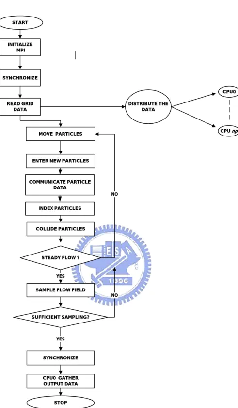
Fig. 2.2 Simplified flow chart of the parallel DSMC method for np processors. ... 44

Fig. 2.3 The additional schemes in the parallel DSMC code. ... 45

Fig. 3.1 The 2D square (L/H) driven cavity flow with moving top plate ... 47

Fig. 3.2 The mesh for Knudsen number 10, 1, 0.1(40×40) ... 48

Fig. 3.3 The mesh for Knudsen number 10, 1, 0.1(100×100). ... 49

Fig. 3.4 The mesh for Knudsen number 0.0033(300×300) ... 50

Fig. 3.4 Properties distribution along vertical line through geometry center (x/L=0.5) (a) u velocity: (b) v velocity: (c) number density: (d) temperature. ... 51

Fig. 3.5 Properties distribution along horizontal line through geometry center (y/L=0.5) (a) u velocity: (b) v velocity: (c) number density: (d) temperature. ... 52

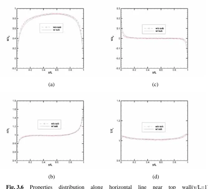
Fig. 3.6 Properties distribution along horizontal line near top wall(y/L=1) (a) u velocity: (b) v velocity: (c) number density: (d) temperature. ... 53

Fig. 3.7 Properties distribution along horizontal line near bottom wall(y/L=0) (a) u velocity: (b) v velocity: (c) number density: (d) temperature. ... 54

Fig. 3.8 Properties distribution along vertical line near left wall(x/L=0) (a) u velocity: (b) v velocity: (c) number density: (d) temperature. ... 55

Fig. 3.9 Properties distribution along vertical line near right wall(x/L=1) (a) u velocity: (b) v velocity: (c) number density: (d) temperature. ... 56

Fig. 3.10 The merit of collision without sub-cells case ... 57

Fig. 3.11 The merit of collision with sub-cells case ... 58

Fig. 3.12 Contour of number density for M = 1.1, (a) Kn = 10; (b) Kn = 1; (c) Kn = 0.1; (d) Kn = 0.01; (e) Kn = 0.0033. ... 59

Fig. 3.13 Contour of temperature for M = 1.1, (a) Kn = 10; (b) Kn = 1; (c) Kn = 0.1; (d) Kn = 0.01; (e) Kn = 0.0033. ... 60

Fig. 3.14 Contour of Mach number for M = 1.1, (a) Kn = 10; (b) Kn = 1; (c) Kn = 0.1; (d) Kn = 0.01; (e) Kn = 0.0033. ... 61

Fig. 3.15 Contour of u-velocity for M = 1.1, (a) Kn = 10; (b) Kn = 1; (c) Kn = 0.1; (d) Kn = 0.01; (e) Kn = 0.0033. ... 62

Fig. 3.16 Contour of v-velocity for M = 1.1, (a) Kn = 10; (b) Kn = 1; (c) Kn = 0.1; (d) Kn = 0.01; (e) Kn = 0.0033. ... 63

Fig. 3.17 Contour of number density for M = 2, (a) Kn = 10; (b) Kn = 1; (c) Kn = 0.1; (d) Kn = 0.01; (e) Kn = 0.0033. ... 64

Fig. 3.18 Contour of temperature for M = 2, (a) Kn = 10; (b) Kn = 1; (c) Kn = 0.1; (d) Kn = 0.01; (e) Kn = 0.0033. ... 65

(11)

(d) Kn = 0.01; (e) Kn = 0.0033. ... 66

Fig. 3.20 Contour of u-velocity for M = 2, (a) Kn = 10; (b) Kn = 1; (c) Kn = 0.1; (d) Kn = 0.01; (e) Kn = 0.0033. ... 67

Fig. 3.21 Contour of v-velocity for M = 2, (a) Kn = 10; (b) Kn = 1; (c) Kn = 0.1; (d) Kn = 0.01; (e) Kn = 0.0033. ... 68

Fig. 3.22 Contour of number density for M = 4, (a) Kn = 10; (b) Kn = 1; (c) Kn = 0.1; (d) Kn = 0.01; (e) Kn = 0.0033. ... 69

Fig. 3.23 Contour of temperature for M = 4, (a) Kn = 10; (b) Kn = 1; (c) Kn = 0.1; (d) Kn = 0.01; (e) Kn = 0.0033. ... 70

Fig. 3.24 Contour of Mach number for M = 4, (a) Kn = 10; (b) Kn = 1; (c) Kn = 0.1; (d) Kn = 0.01; (e) Kn = 0.0033. ... 71

Fig. 3.25 Contour of u-velocity for M = 4, (a) Kn = 10; (b) Kn = 1; (c) Kn = 0.1; (d) Kn = 0.01; (e) Kn = 0.0033. ... 72

Fig. 3.26 Contour of v-velocity for M = 4, (a) Kn = 10; (b) Kn = 1; (c) Kn = 0.1; (d) Kn = 0.01; (e) Kn = 0.0033. ... 73

Fig. 3.27 Contour of number density for Kn = 10, (a) M = 1.1; (b) M = 2; (c) M = 4 .... 74

Fig. 3.28 Contour of temperature for Kn = 10, (a) M = 1.1; (b) M = 2; (c) M = 4 ... 75

Fig. 3.29 Contour of Mach number for Kn = 10, (a) M = 1.1; (b) M = 2; (c) M = 4 ... 76

Fig. 3.30 Contour of u-velocity for Kn = 10, (a) M = 1.1; (b) M = 2; (c) M = 4 ... 77

Fig. 3.31 Contour of v-velocity for Kn = 10, (a) M = 1.1; (b) M = 2; (c) M = 4 ... 78

Fig. 3.32 Contour of number density for Kn = 1, (a) M = 1.1; (b) M = 2; (c) M = 4 ... 79

Fig. 3.33 Contour of temperature for Kn = 1, (a) M = 1.1; (b) M = 2; (c) M = 4 ... 80

Fig. 3.34 Contour of Mach number for Kn = 1, (a) M = 1.1; (b) M = 2; (c) M = 4 ... 81

Fig. 3.35 Contour of u-velocity for Kn = 1, (a) M = 1.1; (b) M = 2; (c) M = 4 ... 82

Fig. 3.36 Contour of v-velocity for Kn = 1, (a) M = 1.1; (b) M = 2; (c) M = 4 ... 83

Fig. 3.37 Contour of number density for Kn = 0.1, (a) M = 1.1; (b) M = 2; (c) M = 4 ... 84

Fig. 3.38 Contour of temperature for Kn = 0.1, (a) M = 1.1; (b) M = 2; (c) M = 4 ... 85

Fig. 3.39 Contour of Mach number for Kn = 0.1, (a) M = 1.1; (b) M = 2; (c) M = 4 ... 86

Fig. 3.40 Contour of u-velocity for Kn = 0.1, (a) M = 1.1; (b) M = 2; (c) M = 4 ... 87

Fig. 3.41 Contour of v-velocity for Kn = 0.1, (a) M = 1.1; (b) M = 2; (c) M = 4 ... 88

Fig. 3.42 Contour of number density for Kn = 0.01, (a) M = 1.1; (b) M = 2; (c) M = 4 . 89 Fig. 3.43 Contour of temperature for Kn = 0.01, (a) M = 1.1; (b) M = 2; (c) M = 4 ... 90

Fig. 3.44 Contour of Mach number for Kn = 0.01, (a) M = 1.1; (b) M = 2; (c) M = 4 ... 91

Fig. 3.45 Contour of u-velocity for Kn = 0.01, (a) M = 1.1; (b) M = 2; (c) M = 4 ... 92

Fig. 3.46 Contour of v-velocity for Kn = 0.01, (a) M = 1.1; (b) M = 2; (c) M = 4 ... 93

Fig. 3.47 Contour of number density for Kn = 0.0033, (a) M = 1.1; (b) M = 2; (c) M = 4 94 Fig. 3.48 Contour of temperature for Kn = 0.0033, (a) M = 1.1; (b) M = 2; (c) M = 4 ... 95

(12)

Fig. 3.50 Contour of u-velocity for Kn = 0.0033, (a) M = 1.1; (b) M = 2; (c) M = 4 ... 97 Fig. 3.51 Contour of v-velocity for Kn = 0.0033, (a) M = 1.1; (b) M = 2; (c) M = 4 ... 98 Fig. 3.52 Effect of Kn for M = 1.1 along vertical line through geometry center with

(a) u-velocity; (b) v-velocity; (c) number density (d) temperature ... 99

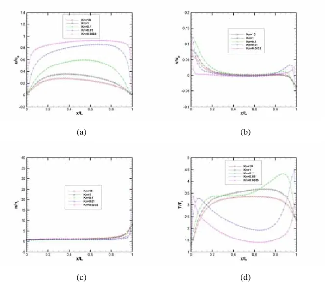
Fig. 3.53 Effect of Kn for M = 1.1 along horizontal line through geometry center with

Fig. 3.54 Effect of Kn for M = 1.1 along horizontal line near top wall(y/L=1) with

Fig. 3.55 Effect of Kn for M = 1.1 along horizontal line near bottom wall(y/L=0) with

Fig. 3.56 Effect of Kn for M = 1.1 along vertical line near left wall(x/L=0) with

Fig. 3.57 Effect of Kn for M = 1.1 along vertical line near right wall(x/L=1) with

Fig. 3.58 Effect of Kn for M = 2 along vertical line through geometry center with

Fig. 3.59 Effect of Kn for M = 2 along horizontal line through geometry center with

Fig. 3.60 Effect of Kn for M = 2 along horizontal line near top wall(y/L=1) with

Fig. 3.61 Effect of Kn for M = 2 along horizontal line near bottom wall(y/L=0) with

Fig. 3.62 Effect of Kn for M = 2 along vertical line near left wall(x/L=0) with

Fig. 3.63 Effect of Kn for M = 2 along vertical line near right wall(x/L=1) with

Fig. 3.64 Effect of Kn for M = 4 along vertical line through geometry center with

Fig. 3.65 Effect of Kn for M = 4 along horizontal line through geometry center with

Fig. 3.66 Effect of Kn for M = 4 along horizontal line near top wall(y/L=1) with

Fig. 3.67 Effect of Kn for M = 4 along horizontal line near bottom wall(y/L=0) with

Fig. 3.68 Effect of Kn for M = 4 along vertical line near left wall(x/L=0) with

Fig. 3.69 Effect of Kn for M = 4 along vertical line near right wall(x/L=1) with

(13)

Fig. 3.71 Effect of M for Kn = 10 along horizontal line through geometry center with

Fig. 3.72 Effect of M for Kn = 10 along horizontal line near top wall(y/L=1) with

Fig. 3.73 Effect of M for Kn = 10 along horizontal line near bottom wall(y/L=0) with

Fig. 3.74 Effect of M for Kn = 10 along vertical line near left wall(x/L=0) with

Fig. 3.75 Effect of M for Kn = 10 along vertical line near right wall(x/L=1) with

Fig. 3.76 Effect of M for Kn = 1 along vertical line through geometry center with

Fig. 3.77 Effect of M for Kn = 1 along horizontal line through geometry center with

Fig. 3.78 Effect of M for Kn = 1 along horizontal line near top wall(y/L=1) with

Fig. 3.79 Effect of M for Kn = 1 along horizontal line near bottom wall(y/L=0) with

Fig. 3.80 Effect of M for Kn = 1 along vertical line near left wall(x/L=0) with

Fig. 3.81 Effect of M for Kn = 1 along vertical line near right wall(x/L=1) with

Fig. 3.82 Effect of M for Kn = 0.1 along vertical line through geometry center with

Fig. 3.83 Effect of M for Kn = 0.1 along horizontal line through geometry center with

Fig. 3.84 Effect of M for Kn = 0.1 along horizontal line near top wall(y/L=1) with

Fig. 3.85 Effect of M for Kn = 0.1 along horizontal line near bottom wall(y/L=0) with

Fig. 3.86 Effect of M for Kn = 0.1 along vertical line near left wall(x/L=0) with

Fig. 3.87 Effect of M for Kn = 0.1 along vertical line near right wall(x/L=1) with

Fig. 3.88 Effect of M for Kn = 0.01 along vertical line through geometry center with

(14)

Fig. 3.90 Effect of M for Kn = 0.01 along horizontal line near top wall(y/L=1) with

Fig. 3.91 Effect of M for Kn = 0.01 along horizontal line near bottom wall(y/L=0) with (a) u-velocity; (b) v-velocity; (c) number density (d) temperature ... 138

Fig. 3.92 Effect of M for Kn = 0.01 along vertical line near left wall(x/L=0) with (a) u-velocity; (b) v-velocity; (c) number density (d) temperature ... 139

Fig. 3.93 Effect of M for Kn = 0.01 along vertical line near right wall(x/L=1) with (a) u-velocity; (b) v-velocity; (c) number density (d) temperature ... 140

Fig. 3.94 Effect of M for Kn = 0.0033 along vertical line through geometry center with (a) u-velocity; (b) v-velocity; (c) number density (d) temperature ... 141

Fig. 3.95 Effect of M for Kn = 0.0033 along horizontal line through geometry center with (a) u-velocity; (b) v-velocity; (c) number density (d) temperature ... 142

Fig. 3.96 Effect of M for Kn = 0.0033 along horizontal line near top wall(y/L=1) with (a) u-velocity; (b) v-velocity; (c) number density (d) temperature ... 143

Fig. 3.97 Effect of M for Kn = 0.0033 along horizontal line near bottom wall(y/L=0) with (a) u-velocity; (b) v-velocity; (c) number density (d) temperature ... 144

Fig. 3.98 Effect of M for Kn = 0.0033 along vertical line near left wall(x/L=0) with (a) u-velocity; (b) v-velocity; (c) number density (d) temperature ... 145

Fig. 3.99 Effect of M for Kn = 0.0033 along vertical line near right wall(x/L=1) with (a) u-velocity; (b) v-velocity; (c) number density (d) temperature ... 146

Fig. 3.100 Streamline for M=1.1 (a) Kn=10; (b) Kn=1; (c) Kn=0.1; (d) Kn=0.01; (e) Kn=0.0033 ... 147

Fig. 3.101 Streamline for M=2 (a) Kn=10; (b) Kn=1; (c) Kn=0.1; (d) Kn=0.01; (e) Kn=0.0033 ... 148

Fig. 3.102 Streamline for M=4 (a) Kn=10; (b) Kn=1; (c) Kn=0.1; (d) Kn=0.01; (e) Kn=0.0033 ... 149

Fig. 3.103 Relative horizontal distance (x/L) of vortex center for various value of Knudsen number and Mach number ... 150

Fig. 3.104 Relative horizontal distance (y/L) of vortex center for various value of Knudsen number and Mach number ... 150

Fig. 3.105 Streamline for Kn=10 (a) M=1.1; (b) M=2; (c) M=4 ... 151

Fig. 3.106 Streamline for Kn=1 (a) M=1.1; (b) M=2; (c) M=4 ... 152

Fig. 3.107 Streamline for Kn=0.1 (a) M=1.1; (b) M=2; (c) M=4 ... 153

Fig. 3.108 Streamline for Kn=0.01 (a) M=1.1; (b) M=2; (c) M=4 ... 154

Fig. 3.109 Streamline for Kn=0.0033 (a) M=1.1; (b) M=2; (c) M=4 ... 155 Fig. 3.110 Relative horizontal distance (x/L) of vortex center for various value of Mach

(15)

Fig. 3.111 Relative horizontal distance (y/L) of vortex center for various value of Mach

number and Knudsen number ... 156

(16)

Nomenclature

λ ：mean free path ρ ：density

σ ：the differential cross section ω ：viscosity temperature exponent Ω : space domain rot ε ：rotational energy v ε ：vibrational energy rot

ζ ：rotational degree of freedom

v

ζ ：vibrational degree of freedom Ut ：time-step

σT ：the total cross section

c ：the total velocity c’ ：random velocity co ：mean velocity

cr ：relative speed

d ：molecular diameter

D ：the throat diameter of the twin-jet interaction dref ：reference diameter

E ：energy

k ：the Boltzmann constant Kn ：Knudsen number

Q

Kn _{: local Knudsen numbers based on flow property Q}

L ：characteristic length; m ：molecule mass

M∞ ：free-stream mach number

n ：number density Re ：Reynolds number To ：stagnation temperature

(17)

T∞ ：free-stream temperature

Tref ：reference temperature

Trot ：rotational temperature

Ttot ：total temperature

Ttr ：translational temperature

Tv ：vibrational temperature

(18)

Chapter 1 Introduction

1.1. Motivation and Background

1.1.1 Importance of Driven Cavity Flows

The driven cavity flow is one of the fundamental fluid flow problems that was often used as the benchmark test problem in computational fluid dynamics. The rationale behind this should be attributed to its simple geometry but having singular points at the corners, which may cause difficulties in numerical simulations. Although they have been thoroughly studied in the literature, most of them were focused on incompressible or continuum compressible regime [Karniadakis, 2001]. Very few researches have been done in the rarefied and near continuum regimes, where the understanding may become important in micro- and nano-scale gas flows that are often encountered in MEMS and NEMS related devices. Further, it may serve as the benchmarking problem for extending a numerical scheme into flow in these regimes, where standard Navier-Stokes equation fails to describe the flow accurately. Thus, an accurate numerical solution of a driven cavity flow in the rarefied and near-continuum regime is strongly required.

(19)

Knudsen number (Kn=λ/L) is a standard parameter that is usually used to indicate the

degree of rarefaction. Note that the mean free path λ is the average distance traveled by molecules before collision and L is the flow characteristic length. In general, flows are

divided into four regimes as follows traditionally: Kn <0.01 (continuum), 0.01<Kn<0.1 (slip

flow), 0.1<Kn<3 (Transitional flow) and Kn>3 (Free molecular flow). Fig. 1.1 (KC Tseng’s

thesis)is a sketch adopted from Bird [Bird’s book, 1994] illustrating the various flow regions and their corresponding solution methods in a dilute gas. In this figure, the local Kn number is

defined with L as the scale length of the macroscopic gradient; that is,

dx d L ρ ρ = . Firstly, the lower bar indicates the continuum formulation. When the local Kn number approaches

zero, the flow reaches inviscid limit and can be solved by Euler equation. As local Kn

increases, molecular nature of the gas becomes dominated. Hence, the Navier-Stoke equation based computational fluid dynamics (CFD) techniques are often used until the Kn approach

0.01. When the Kn larger than 0.01, continuum assumption begins to break down and the

particle-based method is necessary. Secondly, the top bar in this figure indicates the validity of the molecular modeling. It is well known that Boltzmann equation is more appropriate for all flow regimes; however it is rarely used to numerically solve the practical problems because of two major difficulties. They include higher dimensionality (up to seven) of the Boltzmann equation and the difficulties of correctly modeling the integral collision term. As the distance between the molecules increases, collisions between the molecules become less

(20)

and thus neglected, and the flow can be solved by neglecting the collision term of the collisionless Boltzmann equation.

1.1.3 Direct Simulation Monto Carlo Method

An alternative method, known as Direct Simulation Monte Carlo (DSMC), was proposed by Bird to solve the Boltzmann equation using direct simulation of particle collision kinetics, and the associated monograph was published in 1994 [Bird’s book]. Later on, both Nanbu [1986] and Wagner [1992] were able to demonstrate mathematically that the DSMC method is equivalent to solving the Boltzmann equation as the simulated number of particles becomes large. The DSMC method is a particle method for the simulation of gas flows. The gas is modeled at the microscopic level using simulated particles, which each represents a large number of physical molecules or atoms. The physics of the gas are modeled through the motion of particles and collisions between them. Mass, momentum and energy transports between particles are considered at the particle level. The method is statistical in nature and depends heavily upon pseudo-random number sequences for simulation. Physical events such as collisions are handled probabilistically using largely phenomenological models, which are designed to reproduce real fluid behavior when examined at the macroscopic level. This method has become a widely used computational tool for the simulation of gas flows in the Low Kn flow regime, in which molecular effects become important.

(21)

The DSMC method becomes very time-consuming as the flow approaches continuum regime since the sampling cell size has to be much smaller than the local mean free path for the solution to be accurate. Several remedies in speeding up the DSMC computation include: 1) parallel computing [Robinson, 1996-1998]; 2) variable time-step scheme for steady flows [Kannenberg, 2000], and 3) sub-cells within each sampling cell [Bird’s book, 1994]. Details of the “parallel computing” and “variable time-step scheme” can be found in those references cited in the above and are not described here for brevity. Only “sub-cells” concept is described here since it was rarely discussed in detail in the literature. In Bird’s original implementation [see Bird’s book, 1994], number of sub-cells in each sample cell is pre-determined and related sub-cell data are stored in the memory throughout the simulation, which is very costly. This strategy, which enables nearest-neighbor collisions to be enforced, greatly reduces the computational load by increasing the sampling cell size whilst maintaining the same accuracy as compared to that using smaller sampling cell size. Unfortunately, storage of the sub-cell data is memory intensive and inflexible in adjusting the number of sub-cells in each sampling cell during runtime, which may become important in reducing the merit of collision (ratio of mean collision distance to characteristic cell size). Recently, Bird [DS2V code by Bird] has proposed an idea of “transient sub-cells”, which could overcome the above-mentioned shortcomings. However, this idea has been only implemented on structured grids. No report could be found on unstructured grids.

(22)

1.2. Literature Survey

The driven cavity flow is a fluid flow problem that has been very well studied in the continuum limit by using different numerical methods. Ghia, et al. [1982] used the

vorticity-stream function of the 2D incompressible Navier-Stoke equation to study the laminar incompressible flow in a square cavity whose top wall moves with a uniform velocity. The Reynolds number in their study is varied from Re=100 to Re=10,000. They presented the velocity along vertical and horizontal line through geometry center of cavity and the primary vortex position. Erturk, et al. [2005] also utilized the 2D steady incompressible

Navier-Stoke equation with a fine grid. The flow solutions are computed for Re=1000 to Re=21000 with a maximum absolute residuals of the governing equations that were less than 10-10. Until very recently, Stergios, et al. [2005] solved the flow of a rarefied gas in a

rectangular enclosure due to the motion of the upper wall over whose range of the Knudsen number. Their numerical method is base on the 2D linearized BGK kinetic equation with Maxwell diffuse-specular boundary conditions. They presented the simulation data over the whole range of the Knudsen number and various aspect ratio (height/width). However, simulation results by Stergios, et al. [2005] were only good for low speed rarefied gas flows

since the linearized BGK Boltzmann equation was used. In addition, no data were validated by comparing with experiments or solution from direct Boltzmann equation, such as DSMC

(23)

method.

1.3. Specific Objectives of the Thesis

The objectives of the thesis are briefly summarized as follows:

1. To verify the implementation of transient sub-cell technique in a parallelized DSMC code (PDSC) [Wu, et al].

2. To simulate driven cavity flows, including M=1.1-4 of the speed of top driven plate, and Kn=10-0.0033, based on the average number density and wall temperature.

3. To discuss the effects of Knudsen Number and Mach number of the driven plate on the flow fields.

The organization of the thesis is stated as follows. Chapter 1 describes the Introduction, Chapter 2 describes the Numerical Method, Chapter 3 describes the verification of implementation of transient sub-cells, and followed by the Results and Discussion, and finally Chapter 4 describes the conclusion and recommendation of future work..

(24)

Chapter 2 Numerical Method

2.1. The Boltzmann Equation

The Boltzmann equation is one of the most important transport equations in non-equilibrium statistical mechanics, which deals with systems far from thermodynamics equilibrium. There are some assumptions made in the derivation of the Boltzmann equation which defines limits of applicability. They are summarized as follows:

1. Molecular chaos is assumed which is valid when the intermolecular forces are short range. It allows the representation of the two particles distribution function as a product of the two single particle distribution functions.

2. Distribution functions do not change before particle collision. This implies that the encounter is of short time duration in comparison to the mean free collision time. 3. All collisions are binary collisions.

4. Particles are uninfluenced by intermolecular potentials external to an interaction. According to these assumptions, the Boltzmann equation is derived and shown as Eq. (2.1) 4 2 ' ' 1 1 0 ( ) ( ) ( ) ( ) i i c i i i nf nf nf f u F n f f ff g d dU t x u x π σ ∞ −∞ ∂ ∂ ∂ ∂ + + = = − Ω ∂ ∂ ∂ ∂

∫ ∫

(2.1) Meaning of particle phase-space distribution function f is the number of particles with

(25)

range d u , at time t . 3 F is an external force per unit mass and t is the time and _i u is the _i

molecular velocity. σ is the differential cross section and dΩ is an element of solid angle. The prime denotes the post-collision quantities and the subscript 1 denotes the collision partner. Meaning of each term in Eq. (2.1) is described in the following;

1. The first term on the left hand side of the equation represents the time variation of the distribution function of the particles (unsteady term).

2. The second term gives the spatial variation of the distribution function (flux term). 3. The third term describes the effect of a force on the particles (force term).

4. The term at right hand side of the equation is called the collision integral (collision term). It is the source of most of the difficulties in obtaining solutions of the Boltzmann equation.

In general, it is very hard to solve the Boltzmann equation directly using numerical method because the difficulties of correctly modeling the integral collision term. Instead, the DSMC method was used to simulated problems involving rarefied gas dynamics, which is the simulation tool used in the current thesis.

2.2. General Description of the Standard DSMC

According to the expected rarefaction caused by the rarefied gas flows, the direct simulation Monte Carlo (DSMC) method, which is a particle-based method developed by

(26)

Bird during the 1960s, and was widely used as an efficient technique to simulate rarefied gas regime [Bird, 1976 and Bird, 1994]. In the DSMC method, a large number of particles are generated in the flow field to represent real physical molecules rather than a mathematical foundation and it has been proved that the DSMC method is equivalent to solving the Boltzmann equation [Nanbu, 1986 and Wagner, 1992]. The assumptions of molecular chaos and a dilute gas are shared by both the Boltzmann equation and the DSMC method [Bird, 1976 and Bird, 1994]. An important feature of DSMC is that the molecular motion and the intermolecular collisions are uncoupled over the time intervals that are much smaller than the mean collision time. Both the collision between molecules and the interaction between molecules and solid boundaries are computed on a probabilistic basis and, hence, this method makes extensive use of random numbers. In most practical applications, the number of simulated molecules is extremely small as compared to the number of real molecules. The general procedures of the DSMC method are described in the next section, and the consequences of the computational approximations can be found in Bird [Bird, 1976 and Bird, 1994].

In DSMC, there are three popular molecular collision models for real physical behavior and imitate the real particle collision. They include the Hard Sphere (HS), Variable Hard Sphere (VHS) and Variable Soft Sphere (VSS) molecular models [Bird, 1994]. No time counter (NTC) method is often used to determined the probability of collision within a

(27)

samping cell based on the acceptance-rejection method. This method can yield the exact collision rate in both simple gases and gas mixtures, and under either equilibrium or non-equilibrium conditions.

Fig. 2.2 is a general flowchart of the DSMC method. Important steps of the DSMC method include setting up the initial conditions, moving all the simulated particles, indexing (or sorting) all the particles, colliding between particles and sampling the molecules within cells to determine the macroscopic quantities. The details of each step are described in the following:

z Initialization

The first step to use the DSMC method is to set up the geometry and flow conditions. A physical space is discredited into a network of cells and the boundary conditions at domain boundaries have to be assigned according to the flow conditions. An important rule of thumb of selecting the cell size is it should be much smaller than the local mean free path. At the same time the distance of the molecular movement per time step should be smaller than the cell dimension, which is similar to the CFL condition in CFD. After the data of geometry and flow conditions have been read in the code, the number of simulation particles each cell is calculated according to the initial number density and the cell volume. The initial particle velocities are normally assigned to each particle based on the Maxwell-Boltzmann distribution according to the initial velocities and temperature. The position of each particle is

(28)

then randomly allocated within the cell.

z Molecular Movement

After initialization process, the molecule begins move one by one, and the molecule moves in a straight line over the time step. If the particle collides with a solid surface, then it has to reflected back based on the boundary conditions at the surface. If the particle passes through a inflow/outflow boundary, then it has to be removed from the simulation immediately. After the particle reaches its final destination, the cell with which the particle affiliated is recorded.

z Indexing

Relation between particles and cells are reordered according to the order of the increasing particle number in each cell, which is used for collision step.

z Gas Phase Collision

The other most important phase of the DSMC method is the gas phase collision. The DSMC method uses the no time counter (NTC) method to determine the correct collision rate in the collision cell. Number of collision pairs within a cell of volume Vc over a time interval

t

∆ _{is calculated by the following equation:}

c r T N c t V F N N ( ) / 2 1 max∆ σ (2.2)

where N and N are fluctuating and average number of simulated particles, respectively.

N F

(29)

represents. σT _andcr_{are the cross section and the relative speed, respectively. The}

collision probability for each pair of particle chosen can be expressed as

(σTcr)/(σTcr)max (2.3)

Collision is accepted if the above value for the pair is greater than a random fraction. Each cell is treated independently and the collision partners for interactions are chosen randomly, regardless of their positions within the cell. Collision procedures are summarized as follows:

1. Number of collision pairs is calculated according to the NTC method, Eq. (2.2), in each cell.

2. The first particle is chosen randomly from the list of particles within a collision cell.

3. The other collision partner is also chosen randomly within the same cell.

4. The collision is accepted if the computed probability, Eq. (2.3), is greater than a random number.

5. If the collision pair is accepted, then the post-collision velocities are calculated using the mechanics of elastic collision. If the collision pair is not to collide, then proceed to choose the next collision pair.

6. If the collision pair is polyatomic gas, the translational and internal energy can be redistributed by the Larsen-Borgnakke model [1975], which assumes the state is in equilibrium.

(30)

The collision process will be finished until all the collision pairs are handled for all cells and then progress to the next step.

z Sampling

After the particle movement and collision process complete, the particle has updated positions and velocities. Macroscopic flow properties in each cell are assumed to be constant over the cell volume and are sampled from the microscopic properties of all the particles within the cell. Macroscopic properties, including number density, velocities and temperatures, are calculated following the equations as shown below:

nm = ρ _(2.4a) ' c c c c_o = = _o + (2.4b) ) ' ' ' ( 2 1 2 3 2 2 2 w v u m kT_tr = + + (2.4c) ) ( 2 r rot rot k T = ε ζ (2.4d) ) ( 2 v v v k T = ε ζ (2.4e) ) 3 ( ) 3

( tr rot rot v v rot v

tot T T T

T = +ζ +ζ +ζ +ζ (2.4f) where n, m are the number density and molecule mass, receptively. c, co, and c’ are the total

velocity, mean velocity, and random velocity, respectively. In addition, Ttr, Trot, Tv and Ttot are

translational, rotational, vibration and total temperature, respectively. εrot and εv are the

rotational and vibration energy, respectively. ζrot and ζv are the number of degree of

(31)

translational temperature is regarded simply as the total temperature. Vibration effect can be neglect if the temperature of the flow is low enough.

The flow will be monitored if steady state is reached. If the flow is still in the transient phase, then sampling of the properties should be reset until the flow reaches steady state. As the flow reaches physically steady state, time averaging in each cell is used to obtain macroscopic properties in each cell. As a rule of thumb, sampling of particles starts when the number of molecules in the calculation domain becomes approximately constant.

2.3. General Description of the PDSC

In the past few years, we have developed a parallelized direct simulation Monte Carlo code, named PDSC, which is portable on distributed memory machines. Important features of the PDSC code can be found in the references [Wu et al.’s JCP paper, 2006; JCP paper submitted in June 2007; JFM paper under preparation, 2007] and only several of them are briefly described in the following.

1) 2D/2D-axisymmetric/3-D unstructured-grid topology: PDSC can accept either 2D/2D-axisymmetric (triangular, quadrilateral or hybrid triangular-quadrilateral) or 3D (tetrahedral, hexahedral or hybrid tetrahedral-hexahedral) mesh [Wu et al.’s JCP paper, 2006]. Computational cost of particle tracking for the unstructured mesh is generally higher than that for the structured mesh. However, the use of the unstructured mesh, which provides excellent flexibility of handling boundary conditions with complicated geometry and of parallel computing using dynamic domain decomposition based on load balancing, is highly justified.

(32)

2) Parallel computing using dynamic domain decomposition: Load balancing of PDSC is achieved by repeatedly repartitioning the computational domain using a multi-level graph-partitioning tool, PMETIS [Wu and Tseng, 2005], by taking advantage of the unstructured mesh topology employed in the code. A decision policy for repartition with a concept of Stop-At-Rise (SAR) [Wu and Tseng, 2005] or constant period of time (fixed number of time steps) can be used to decide when to repartition the domain. Capability of repartitioning of the domain at constant or variable time interval is also provided in PDSC. Resulting parallel performance is excellent if the problem size is comparably large. Details can be found in Wu and Tseng [Wu and Tseng, 2005].

3) Spatial variable time-step scheme: PDSC employs a spatial variable time-step scheme (or equivalently a variable cell-weighting scheme), based on particle flux (mass, momentum, energy) conservation when particles pass interface between cells. This strategy can greatly reduce both the number of iterations towards the steady state, and the required number of simulated particles for an acceptable statistical uncertainty. Past experience shows this scheme is very effective when coupled with an adaptive mesh refinement technique [Wu et al.’s CPC paper, 2004].

4) Unsteady flow simulation: An unsteady sampling routine is implemented in PDSC, allowing the simulation of time-dependent flow problems in the near continuum range [JCP paper submitted in June 2007]. A post-processing procedure called DSMC Rapid Ensemble Averaging Method (DREAM) is developed to improve the statistical scatter in the results while minimizing both memory and simulation time. In addition, a temporal variable time-step (TVTS) scheme is also developed to speed up the unsteady flow simulation using PDSC. More details can be found in [JCP paper submitted in June 2007].

(33)

5) Transient Sub-cells: Recently, transient sub-cells are implemented in PDSC directly on the unstructured grid, in which the nearest-neighbor collision can be enforced, whilst maintaining minimal computational overhead [JFM paper under preparation, 2007]. Details of the idea and implementation are described next.

2.4. Transient Sub-Cells for PDSC

[JFM paper under preparation, 2007]

The implementation of sub-cells in DSMC allows the maintenance of good collision quality within the simulation, even for grids which are “under-resolved” (that is, if the sampling cells are bigger than the recommended setting of 1/3~ 1/2 times the local mean free path). Running simulations with under-resolved sampling cells which employ sub-cells results in a reduction in the computational and memory requirements of the simulation, albeit at the cost of a reduction in the possible sampling resolution of the macroscopic properties, but without sacrificing simulation accuracy.

In PDSC, unstructured grids are used, requiring an adaptation of the transient sub-cells scheme, which was originally promoted by Bird [DS2V code by Bird]. In PDSC, the sampling cells are divided into sub-cells during the collision routine. Because the sub-cells only exist in one sampling cell at a time, and only during the collision routine, they can be considered “transient sub-cells” which will have negligible computer memory overhead. In every case, these sub-cells are quadrilateral in 2D or hexahedral in 3D which reduces the complexity of sub-dividing the sampling cell and greatly facilitates particle indexing. The size of the sub-cells is indirectly controlled by the user, who inputs the desired averaged number of

(34)

particles per sub-cell, P. The program then determines the dimensions of the sub-cell array based on the number of particles with the cell, Nparts. Briefly, the total number of sub-cells are

computed by the rule for the 2-D case

parts parts

N N

P × P

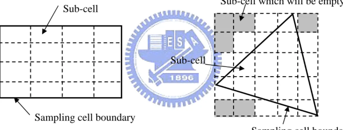
_(2.21) Fig. 2.4 shows the way in which both rectangular and triangular sampling cells are

divided into sub-cells. As can be seen, in the unstructured case, there may be sub-cells which are entirely outside the boundary of the sampling cell, however this has no affect on the collision routine. In both cases, the concept is easily extended to three-dimensional sampling cells.

During the collision routine, a particle is chosen at random from some point within the whole sampling cell. The sub-cell in which the particle lies is then determined and if another particle is in the same sub-cell then these particles are chosen for collision. If the first particle is alone within the sub-cell, then adjacent sub-cells are scanned for a collision partner. These sub-cell routines ensure nearest neighbor collisions, even within under-resolved sampling cells, with minimal computational and memory overhead.

Bird has also shown that preventing particles from colliding again their last collision partner, reduces the error in some variables such as heat transfer and shear stress by up to 5% [ref-Bird manual of DS2V code]. The basis of this is that collisions between particles which just collided with each other is unphysical, since the particle must be moving away from each

(35)

other after the first collision. A minor modification was made to PDSC to prevent particles colliding with their last collision partner. This involved the creation of an array in which the last collision partner for every particle is stored and if the two particles are subsequently chosen for collision without having collided with any other particle, the collision is rejected.

(36)

Chapter 3 Results and Discussion

3.1 Benchmark of Transient Sub-cell Method

Although this thesis is concerned with supersonic square driven cavity flows in rarefied regime, a subsonic flow case with M=0.5 and Kn=0.01 is used as the benchmark case. The rationale is that a subsonic flow represents a more stringent test problem than a supersonic flow for the DSMC method in terms of statistical uncertainties.

3.1.1 Problem Description and Test Conditions

Flow and simulation conditions are summarized in Table I. Fig. 3.1 sketches the 2D square driven cavity flow. PDSC simulations are conducted, respectively, using a coarse mesh (100×100 cells, 100 particles per cell) with transient sub-cells and a finer mesh (400×400 cells, 25 particles per cell) without transient sub-cells. Results using the finer mesh are considered to be a benchmark solution since the simulation conditions satisfy all requirements for a good DSMC computation. Since the overhead of indexing the particles using transient sub-cells is minimal (at most 15% as compared to that without using transient sub-cells if less than 100 particles per cell), resulting computational time using transient sub-cells is about only 1/4 of that without transient sub-cells, considering the similar accuracy of DSMC

(37)

simulations, which is shown next. If 100 particles per cell is used in the case without transient sub-cells, more benefit of computational time can gained by using transient sub-cells.

3.1.2 Simulation Results of Benchmark

Fig. 3.5 (a)-(d) (a)-(d) present the profiles of various properties ((a) u-velocity, (b) v-velocity, (c)number density and (d)temperature) along the central vertical line (x/L=0.5). In these figures, up and L represents the top plate speed and length (also width) of the driven

cavity, respectively. Results show that simulation data with and without transient sub-cells are in good agreement considering the inherent statistical uncertainties of the DSMC method. Statistical uncertainties with transient sub-cells are even lower than those without transient sub-cells, especially for the v velocity, which is generally low as compared to the u velocity along the x/L=0.5 line. It clearly demonstrates that with transient sub-cells accuracy of DSMC simulation can be well preserved using cell size even close to local mean path. Similar trends can be found in Fig. 3.6 (a)-(d), in which the profiles of various properties are presented along the central horizontal line (y/L=0.5). In the simulation, desired averaged number of particles per sub-cell, P, is set to be 1. Not unexpectedly, the merit of collision (=mean collision distance/local mean free path), which represents the quality of collisions in a DSMC simulation, is generally much smaller by using transient sub-cells than that without using transient sub-cells, as illustrated in Fig. 3.11 and Fig. 3.12. Bird [???] has argued that the

(38)

merit of collision in the range of 0.1~0.2 represents a good DSMC simulation. Result show that the simulation used coarse mesh with transient sub-cell approximate that used finer mesh without transient sub-cell. Therefore, the simulation with transient sub-cell keeping minimal computational overhead and memory requirement simultaneously, but still has simulation accuracy.

3.2 Simulation Results of Driven Cavity Flows

According to previous section, we have found the transient sub-cell method can greatly reduce the computational cost and still has good quality of solution. In this section, we have used this technique in PDSC to simulate steady supersonic square driven cavity flows in a systematic way. Thus, we can understand more about the effects of rarefaction and compressibility in such conditions.

3.2.1 Problem Description and Test Conditions

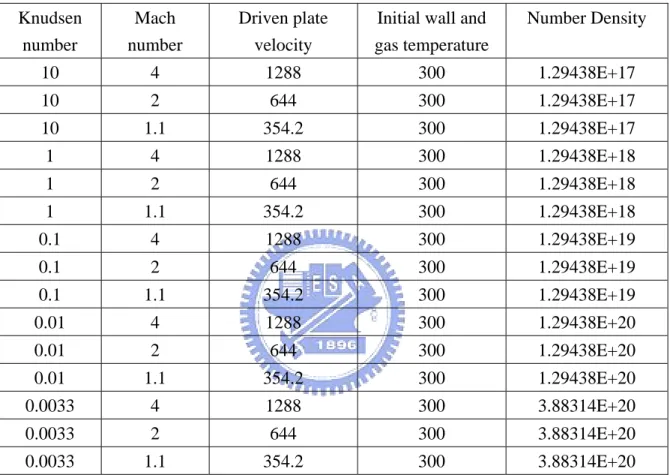
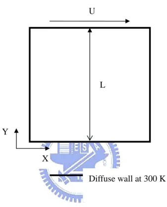
Fig. 3.1 shows the sketch of the 2D square (L/H=1) driven cavity flow with moving top plate. Flow and simulation conditions are summarized in Table II and Table III. Argon is used as the working gas, while the initial temperatures inside the cavity and wall temperatures are set as 300K. Mach number and Knudsen number (based on wall temperature and width of the cavity) is in the range of 1.1-4 and 10-0.0033. Uniform mesh distribution is used

(39)

throughout the present study for all cases.

3.2.2 Effects of Knudsen Number

In this section, we were observed effects of Knudsen number in the same Mach number (Ma=1.1-4). We were showed general simulation results include density, velocity in the x-direction, velocity in the y-direction, temperature, Mach number, and streamline. We were showed property distributions across cavity centroid for x/L = 0.5, y/L = 0 to 1 and y/L = 0.5, x/L = 0 to 1. We showed property distributions near the solid walls. Finally, we were observed the recirculation center position in different cases.

3.2.2.1 General Simulation Results

Fig. 3.23 shows that number density contour for Ma=4, and Knudsen number 10, 1, 0.1, 0.01 and 0.0033 respectively. Driven plate takes particles to the right-hand upper corner. An ultra high-density region appears at the very right-hand upper corner due to the high-speed moving plate at the top of the cavity. Therefore the particles are larger than initial value. In addition, there are low densities at the left-hand upper corner. In the other series, fixed M=1.1 and M=2 are showed in Fig. 3.13 and Fig. 3.18.

Fig. 3.24 show that temperature contour for Ma=4, and Knudsen number 10, 1, 0.1, 0.01 and 0.0033 respectively. We normalize temperature to divide the initial temperature 300K.

(40)

There are two ultra temperatures region in the cavity. One of them is the right-hand upper corner which temperature increased as a result of density increased; the other one is left-hand upper corner which temperature increased due to high vertical speed. Finally, the temperature increase more seriously as Knudsen number decreased. In the other series, fixed M=1.1 and M=2 are showed in Fig. 3.14 and Fig. 3.19.

Fig. 3.25 show that Mach contour for Ma=4, and Knudsen number 10, 1, 0.1, 0.01 and 0.0033 respectively. In the other series, fixed M=1.1 and M=2 are showed in Fig. 3.15 and Fig. 3.20.

Fig. 3.26 show that u-velocity contour for Ma=4, and Knudsen number 10, 1, 0.1, 0.01 and 0.0033 respectively. The maximum u-velocity values are 0.3, 0.35, 0.55, 0.8, and 0.9 with Knudsen number 10, 1, 0.1, 0.01 and 0.0033, respectively. Because of rarefaction effect caused slip phenomenon and the slip velocity along the solid walls increase with Knudsen number at the same Mach number. We normalize u-velocity to divide the upper plate velocity. The velocity more and more decrease when Knudsen number increase. In the other series, fixed M=1.1 and M=2 are showed in Fig. 3.16 and Fig. 3.21.

Fig. 3.27 show that v-velocity contour for Ma=4, and Knudsen number 10, 1, 0.1, 0.01 and 0.0033 respectively. We normalize v-velocity to divide the upper plate velocity. An ultra high-speed region appears at the left-hand and right-hand upper region. In the other series, fixed M=1.1 and M=2 are showed in Fig. 3.17 and Fig. 3.22.

(41)

As mentioned above, we can be briefly summarized as follows:

1. The slip velocity more and more decrease when Knudsen number increase.

2. An ultra high-density region appears at the very right-hand upper corner due to the high-speed moving plate at the upper of the cavity

3. There are two ultra temperatures region in the right and left corner in cavity.

3.2.2.2 Property Distributions Across Cavity Centroid

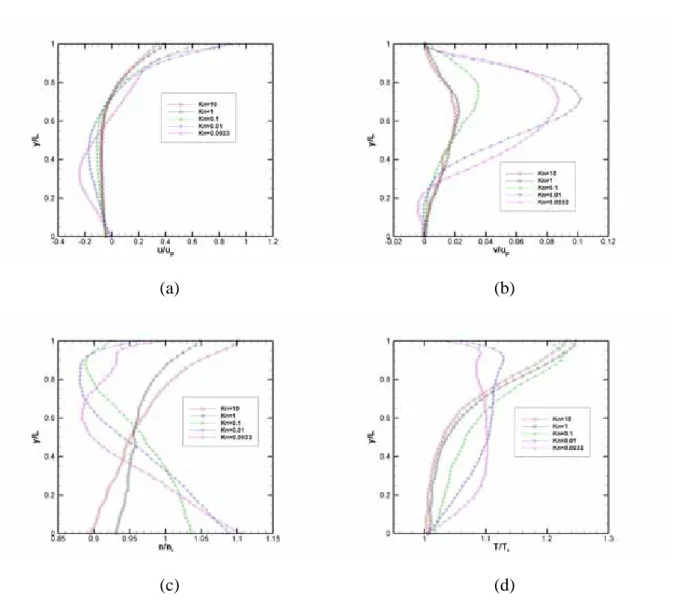
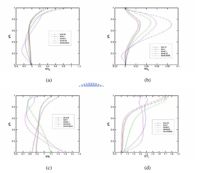
Fig. 3.65 (a)-(d) present the profiles of various properties ((a) u-velocity, (b) v-velocity, (c)number density and (d)temperature) along vertical line through geometry center(x/L=0.5) for Ma=4, and Knudsen number 10, 1, 0.1, 0.01 and 0.0033 respectively. In the other series, fixed M=1.1 and M=2 are showed in Fig. 3.53 and Fig. 3.59.

Fig. 3.66 (a)-(d) present the profiles of various properties ((a) u-velocity, (b) v-velocity, (c)number density and (d)temperature) along horizontal line through geometry center(y/L=0.5) for Ma=4, and Knudsen number 10, 1, 0.1, 0.01 and 0.0033 respectively. In the other series, fixed M=1.1 and M=2 are showed in Fig. 3.54 and Fig. 3.60.

3.2.2.3 Property Distributions Near Solid Walls

Usually, the simulation data save in the cell center for DSMC technique. Thus, observation cell center data properties are average and correct. The positions are show in Table IV. Fig. 3.67

(42)

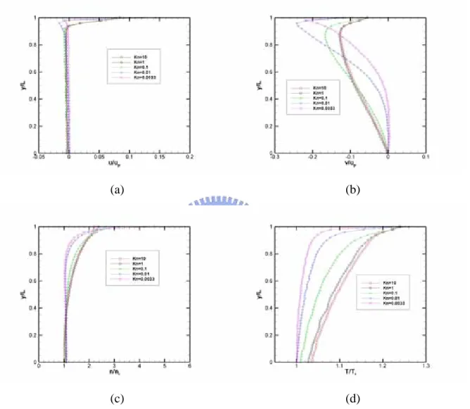
(a)-(d) present the profiles of various properties ((a) u-velocity, (b) v-velocity, (c)number density and (d)temperature) along horizontal line near top wall(y/L=1) for Ma=4, and Knudsen number 10, 1, 0.1, 0.01 and 0.0033 respectively. In the other series, fixed M=1.1 and M=2 are showed in Fig. 3.55 and Fig. 3.61.

Fig. 3.68 (a)-(d) present the profiles of various properties ((a) u-velocity, (b) v-velocity, (c)number density and (d)temperature) along horizontal line near bottom wall(y/L=0) for Ma=4, and Knudsen number 10, 1, 0.1, 0.01 and 0.0033 respectively. In the other series, fixed M=1.1 and M=2 are showed in Fig. 3.56 and Fig. 3.62.

Fig. 3.69 (a)-(d) present the profiles of various properties ((a) u-velocity, (b) v-velocity, (c)number density and (d)temperature) along vertical line near left wall(x/L=0) for Ma=4, and Knudsen number 10, 1, 0.1, 0.01 and 0.0033 respectively. In the other series, fixed M=1.1 and M=2 are showed in Fig. 3.57 and Fig. 3.63.

Fig. 3.70 (a)-(d) present the profiles of various properties ((a) u-velocity, (b) v-velocity, (c)number density and (d)temperature) along vertical line near right wall(x/L=1) for Ma=4, and Knudsen number 10, 1, 0.1, 0.01 and 0.0033 respectively. In the other series, fixed M=1.1 and M=2 are showed in Fig. 3.58 and Fig. 3.64.

3.2.2.4 Recirculation Center Position

(43)

0.0033 respectively. There are only one vortex for Kn=10, 1 and 0.1, but it has the additional second vortex at the right bottom corner for Kn=0.01 and 0.0033. Fig. 3.101 shows the streamline of M=2 and Knudsen number 10, 1, 0.1, 0.01 and 0.0033 respectively. Identically, it has the additional second vortex at the right bottom corner. Besides, the second vortex appear for Kn=10. Fig. 3.102 shows the streamline of M=4 and Knudsen number 10, 1, 0.1, 0.01 and 0.0033 respectively. It has second vortex in all case besides Kn=0.1.

Fig. 3.103 shows the relative horizontal distance (x/L) of the vortex center for various values of Knudsen number and Mach number. Result show that the vertex center position has no obvious regular in x-direction. Fig. 3.103 shows the relative vertical distance (y/L) of the vortex center for various values of Knudsen number and Mach number. It shows that the vortex center move down as decreasing Knudsen number for M=2 and 4; but it has no regular for M=1.1.

3.2.3 Effects of Mach Number of the Driven Plate

In this section, we were observed effects of Mach number in the same Knudsen number (Kn=10-0.0033). We were showed general simulation results include density, velocity in the x-direction, velocity in the y-direction, temperature, Mach number, and streamline. We were showed property distributions across cavity centroid for x =0.5m, y= 0 to 1m and y=0.5m, x=0 to 1m. We showed property distributions near the solid walls. Finally, we were observed

(44)

the recirculation center position in different cases.

3.2.3.1 General Simulation Results

3.2.3.1.1 High Kn Regime (Kn=10, 1, 0.1)

Fig. 3.28 shows that number density contour for Kn=10, and Mach number 1.1, 2 and 4 respectively. Driven plate takes particles to the right-hand upper corner. An ultra high-density region appears at the very right-hand upper corner due to the high-speed moving plate at the top of the cavity. In addition, there is low density at the left-hand upper corner. The max number density reaches 2.2, 4.2 and 7.5 times the initial value as M = 1.1, 2 and 4 respectively. In the other series, fixed Kn=1 and Kn=0.1 are showed in Fig. 3.33 and Fig. 3.38.

Fig. 3.29 shows that temperature contour for Kn=1, and Mach number 1.1, 2 and 4 respectively. We normalize temperature to divide the initial temperature 300K. Temperature near the top plate increases with increasing driven plate velocity. Besides, the temperature increase more seriously as Mach number increased. In the other series, fixed Kn=1 and Kn=0.1 are showed in Fig. 3.34 and Fig. 3.39.

Fig. 3.30 shows that Mach number contour for Kn=0.1, and Mach number 1.1, 2 and 4 respectively. The velocity near the top plate is lower compared with the top plate velocity; it is just about 0.3 times the velocity of driven plate. In the other series, fixed Kn=1 and

(45)

Kn=0.1are showed in Fig. 3.35 and Fig. 3.40.

Fig. 3.31 shows that u-velocity contour for Kn=0.01, and Mach number 1.1, 2 and 4 respectively. We normalize temperature to divide the initial driven plate velocity. The maximum u-velocity values are all about 0.3. Because of rarefaction effect caused slip phenomenon and the velocity remain the 0.3 times the top plate velocity. In the other series, fixed Kn=1 and Kn=0.1 are showed in Fig. 3.36 and Fig. 3.41.

Fig. 3.32 shows that v-velocity contour for Kn=0.0033, and Mach number 1.1, 2 and 4 respectively. We normalize v-velocity to divide the upper plate velocity. An ultra high-speed region appears at the left-hand and right-hand upper region. In the other series, fixed Kn=1 and Kn=0.1 are showed in Fig. 3.37 and Fig. 3.42.

3.2.3.1.2 Low Kn Regime (Kn=0.01, 0.0033)

Fig. 3.42 shows that number density contour for Kn=0.01, and Mach number 1.1, 2 and 4 respectively. In this regime, the region of influence is about all domain. An ultra high-density region appears at the very right-hand upper corner. the number density of sides of the cavity is larger than inside of the cavity, besides it near the top plate. The max number density reaches 3, 7 and 15 times the initial value as M = 1.1, 2 and 4 respectively. When increasing Mach number, the phenomenon is acuter. In the other series, fixed Kn=0.0033 is showed in Fig. 3.48.

(46)

Fig. 3.43 shows that temperature contour for Kn=0.01, and Mach number 1.1, 2 and 4 respectively. We normalize temperature to divide the initial temperature 300K. Temperature near the top plate increases with increasing driven plate velocity. Besides, the temperature increase more seriously as Mach number increased. In the other series, fixed Kn=0.0033 is showed in Fig. 3.49.

Fig. 3.44 shows that Mach number contour for Kn=0.01, and Mach number 1.1, 2 and 4 respectively. Compare the velocity near the top plate with the top plate is much lower, it is 0.8 times the velocity of driven plate. In the other series, fixed Kn=0.0033 is showed in Fig. 3.50.

Fig. 3.45 shows that u-velocity contour for Kn=0.01, and Mach number 1.1, 2 and 4 respectively. We normalize temperature to divide the initial driven plate velocity. The maximum u-velocity values are all about 0.8. Because of rarefaction effect caused slip phenomenon and the velocity reduces 20％ of the top plate velocity. In the other series, fixed Kn=0.0033 is showed in Fig. 3.51.

Fig. 3.46 shows that v-velocity contour for Kn=0.01, and Mach number 1.1, 2 and 4 respectively. We normalize v-velocity to divide the upper plate velocity. An ultra high-speed region appears at the left-hand and right-hand upper region. In the other series, fixed Kn=0.0033 is showed in Fig. 3.52.

(47)

3.2.3.2 Property Distributions Across Cavity Centroid

3.2.3.2.1 High Kn Regime (Kn=10, 1, 0.1)

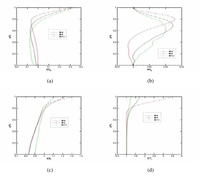
Fig. 3.75 (a)-(d) present the profiles of various properties ((a) u-velocity, (b) v-velocity, (c)number density and (d)temperature) along vertical line through geometry center(x/L=0.5) for Kn = 10, and Mach number 1.1, 2 and 4 respectively.

Fig. 3.76 (a)-(d) present the profiles of various properties ((a) u-velocity, (b) v-velocity, (c)number density and (d)temperature) along horizontal line through geometry center(y/L=0.5) for Kn = 10, and Mach number 1.1, 2 and 4 respectively.

3.2.3.2.2 Low Kn Regime (Kn=0.01, 0.0033)

Fig. 3.88 (a)-(d) present the profiles of various properties ((a) u-velocity, (b) v-velocity, (c)number density and (d)temperature) along vertical line through geometry center(x/L=0.5) for Kn = 0.01, and Mach number 1.1, 2 and 4 respectively.

Fig. 3.89 (a)-(d) present the profiles of various properties ((a) u-velocity, (b) v-velocity, (c)number density and (d)temperature) along horizontal line through geometry center(y/L=0.5) for Kn = 0.01, and Mach number 1.1, 2 and 4 respectively.

(48)

3.2.3.3 Property Distributions Near Solid Walls

3.2.3.3.1 High Kn Regime (Kn=10, 1, 0.1)

Usually, the simulation data save in the cell center for DSMC technique. Thus, observation cell center data properties are average and correct. The positions are show in Table IV. Fig. 3.72 (a)-(d) present the profiles of various properties ((a) u-velocity, (b) v-velocity, (c)number density and (d)temperature) along horizontal line near top wall (y/L=1) for Kn = 10, and Mach number 1.1, 2 and 4 respectively. Fig. 3.76 and Fig. 3.82 change the Mach number as 1 and 0.1, respectively.

Fig. 3.73 (a)-(d) present the profiles of various properties ((a) u-velocity, (b) v-velocity, (c)number density and (d)temperature) along horizontal line near bottom plate (y/L=0) for Kn = 10, and Mach number 1.1, 2 and 4 respectively. Fig. 3.77 and Fig. 3.83 change the Mach number as 1.1 and 2, respectively.

Fig. 3.74 (a)-(d) present the profiles of various properties ((a) u-velocity, (b) v-velocity, (c)number density and (d)temperature) along vertical line near left wall(x/L=0) for Kn = 10, and Mach number 1.1, 2 and 4 respectively. Fig. 3.77 and Fig. 3.83 change the Mach number as 1.1 and 2, respectively.

Fig. 3.75 (a)-(d) present the profiles of various properties ((a) u-velocity, (b) v-velocity, (c)number density and (d)temperature) along vertical line near right wall(x/L=1) for Kn = 10, and Mach number 1.1, 2 and 4 respectively. Fig. 3.77 and Fig. 3.83 change the Mach number

(49)

as 1.1 and 2, respectively.

3.2.3.3.2 Low Kn Regime (Kn=0.01, 0.0033)

Fig. 3.89 (a)-(d) present the profiles of various properties ((a) u-velocity, (b) v-velocity, (c)number density and (d)temperature) along horizontal line near top wall (y/L=1) for Kn = 0.01, and Mach number 1.1, 2 and 4 respectively. Fig. 3.76 and Fig. 3.82 change the Mach number as 1 and 0.1, respectively.

Fig. 3.90 (a)-(d) present the profiles of various properties ((a) u-velocity, (b) v-velocity, (c)number density and (d)temperature) along horizontal line near bottom wall(y/L=0) for Kn = 0.01, and Mach number 1.1, 2 and 4 respectively. Fig. 3.77 and Fig. 3.83 change the Mach number as 1.1 and 2, respectively.

Fig. 3.91 (a)-(d) present the profiles of various properties ((a) u-velocity, (b) v-velocity, (c)number density and (d)temperature) along vertical line near left wall(x/L=0) for Kn = 0.01, and Mach number 1.1, 2 and 4 respectively. Fig. 3.77 and Fig. 3.83 change the Mach number as 1.1 and 2, respectively.

Fig. 3.92 (a)-(d) present the profiles of various properties ((a) u-velocity, (b) v-velocity, (c)number density and (d)temperature) along vertical line near right wall(x/L=1) for Kn = 0.01, and Mach number 1.1, 2 and 4 respectively. Fig. 3.77 and Fig. 3.83 change the Mach number as 1.1 and 2, respectively.

以平行化直接模擬蒙地卡羅法模擬自由分子流到近連續流的空穴超音速流場

國 立 交 通 大 學

機

械

工

程

學

系

碩士論文

以平行化直接模擬蒙地卡羅法模擬自由分子流到近連續流的空穴

超音速流場

Parallel Monte Carlo Simulation of Supersonic Driven Cavity

Flows from Free-molecular to Near-continuum Regime

研 究 生：謝昇汎

指導教授：吳宗信 博士

致謝

以平行化直接模擬蒙地卡羅法模擬自由分子流到近連續流的空穴

超音速流場

學生: 謝昇汎 指導教授: 吳宗信

國立交通大學機械工程學系

摘要

Parallel Monte Carlo Simulation of Supersonic Driven-Cavity Flow from

Free-molecular to Near-continuum Regime

Student : Sheng-Fan Hsien Advisor : Dr. Jong-Shinn Wu

Department of Mechanical Engineering

National Chiao-Tung University

Abstract

List of Tables

Table of Contents

List of Figures

Nomenclature

Chapter 1

Introduction

1.1. Motivation and Background

1.1.1 Importance of Driven Cavity Flows

1.1.3 Direct Simulation Monto Carlo Method

1.2. Literature Survey

1.3. Specific Objectives of the Thesis

Chapter 2

Numerical Method

2.1.

The Boltzmann Equation

∫ ∫

2.2.

General Description of the Standard DSMC

2.3.

General Description of the PDSC

2.4.

Transient Sub-Cells for PDSC

Chapter 3

Results and Discussion

3.1

Benchmark of Transient Sub-cell Method

3.1.1 Problem Description and Test Conditions

3.1.2 Simulation Results of Benchmark

3.2

Simulation Results of Driven Cavity Flows

3.2.1

Problem Description and Test Conditions

3.2.2

Effects of Knudsen Number

3.2.2.1 General Simulation Results

3.2.2.2 Property Distributions Across Cavity Centroid

3.2.2.3 Property Distributions Near Solid Walls

3.2.2.4 Recirculation Center Position

3.2.3

Effects of Mach Number of the Driven Plate

3.2.3.1 General Simulation Results

3.2.3.1.1 High Kn Regime (Kn=10, 1, 0.1)

3.2.3.1.2 Low Kn Regime (Kn=0.01, 0.0033)

3.2.3.2 Property Distributions Across Cavity Centroid

3.2.3.2.1 High Kn Regime (Kn=10, 1, 0.1)

3.2.3.2.2 Low Kn Regime (Kn=0.01, 0.0033)

3.2.3.3 Property Distributions Near Solid Walls

3.2.3.3.1 High Kn Regime (Kn=10, 1, 0.1)

3.2.3.3.2 Low Kn Regime (Kn=0.01, 0.0033)

國立交通大學

研究生：謝昇汎

指導教授：吳宗信博士

學生: 謝昇汎指導教授: 吳宗信