相依製程上平均值和變異數過度調整之適應性管制(II)

行政院國家科學委員會專題研究計畫 成果報告

相依製程上平均值和變異數過度調整之適應性管制(2/2)

研究成果報告(完整版)

計 畫 類 別 ： 個別型 計 畫 編 號 ： NSC 95-2118-M-004-002- 執 行 期 間 ： 95 年 08 月 01 日至 97 年 01 月 31 日 執 行 單 位 ： 國立政治大學統計學系 計 畫 主 持 人 ： 楊素芬 計畫參與人員： 碩士班研究生-兼任助理：余譽寧、陳琬昀 大學生-兼任助理：高義明、陳昭如 報 告 附 件 ： 出席國際會議研究心得報告及發表論文 處 理 方 式 ： 本計畫涉及專利或其他智慧財產權，2 年後可公開查詢

中 華 民 國 97 年 03 月 04 日

行政院國家科學委員會補助專題研究計畫

_■

成 果 報 告

期中進度報告

相依製程上平均值和變異數過度調整之適應性管制

計畫類別：

■

個別型計畫 □ 整合型計畫

計畫編號：NSC 95－2118－M－004－002－

執行期間： 94 年 8 月 1 日至 97 年 1 月 31 日

計畫主持人：楊素芬教授

共同主持人：

計畫參與人員：

成果報告類型(依經費核定清單規定繳交)：□精簡報告

■

完整報告

本成果報告包括以下應繳交之附件：

□赴國外出差或研習心得報告一份

□赴大陸地區出差或研習心得報告一份

■

出席國際學術會議心得報告及發表之論文各一份

□國際合作研究計畫國外研究報告書一份

處理方式：除產學合作研究計畫、提升產業技術及人才培育研究計畫、

列管計畫及下列情形者外，得立即公開查詢

□涉及專利或其他智慧財產權，□一年

■

二年後可公開查詢

執行單位：政 治 大 學 統 計 系

中 華 民 國 97 年 3 月 6 日

II

I have finished about 6papers written for the 2 years project. It is impossible to put all the papers in the file., so just put 3 papers in.

USING VSI EWMA CHARTS TO MONITOR DEPENDENT PROCESS STEPS WITH INCORRECT ADJUSTMENT

Su-Fen Yang Yi-Ning Yu Department of Statistics National Chengchi University, Taiwan

e-mail:yang@nccu.edu.tw

ABSTRACT

The article considers the variable process control scheme for two dependent process steps with incorrect adjustment. Incorrect adjustment of a process may result in shifts in process mean, ultimately affecting the quality of products. We construct variable sampling interval (VSI)EWMA and _ZX EWMA control charts to effectively monitor the _Ze

quality variable produced by the first process step with incorrect adjustment and the quality variable produced by the second process step with incorrect adjustment. The performance of the proposed VSI control charts is measured by the adjusted average time to signal (AATS) derived using a Markov chain approach. An example of the automobile braking

system with incorrect adjustment shows the application and performance of the proposed

VSI EWMA_ZX and EWMA control charts in detecting shifts in process mean. _Ze

Furthermore, the performance of the proposed VSI

X

Z

EWMA and

e

Z

EWMA control charts

and the fixed sampling interval (FSI) EWMA_ZX and EWMA control charts are _Ze

compared by numerical analysis results. These demonstrate that the former is much faster in detecting small and median shifts in mean. The optimum VSI EWMA and _ZX EWMA _Ze

control charts are also proposed using optimization technique when quality engineers cannot specify the values of variable sampling intervals. It has been found that the optimum

VSI EWMA and_ZX EWMA control charts always work better than the VSI_Ze EWMA _ZX

and

e

Z

EWMA control charts.

Key words: Control charts; dependent process steps; incorrect adjustment; Markov chain.

1. INTRODUCTION

Control charts are important tools in statistical quality control. They are used to effectively monitor and determine whether a process is in-control or out-of-control. A common problem in statistical process control is process adjusted unnecessarily (or overadjustment of a process) (see Deming, 1982) due to incorrect use of control chart by the operator or since the only information about the state of the process is available through sampling. A process requires adjustment, when a control chart indicates that it is out of

III

control. However, the process may be adjusted unnecessarily, when a false alarm occurs. Woodall (1986) noted that the effect of overadjustment is a quite significant increase in variability of the quality characteristic. Collani and Saniga (1994) proposed an adjustment model for theX control chart with a single special cause that considers the effects of

process with incorrect adjustment from economic viewpoint. Their model determines the optimal design parameters of the X control chart which maximize the profitability of the

process. Yang and Yang (2004) addressed the economic adjustment model for X control

chart with multiple special causes.

However, the above papers, even Shewhart X control charts, always monitor a process by taking equal samples of size at a fixed sampling interval (FSI), they are usually slow in signaling small to moderate shifts in the process mean. Consequently, several alternatives have been developed to improve the performance of X control charts in recent years. One of the useful approaches to improve the detecting ability is to use a variable sampling interval (VSI) control chart instead of the traditional FSI. Whenever there is some indication that a process parameter may have changed, the next sampling interval should be shorter. On the other hand, if there is no indication of a parameter change, then the next sampling interval should be longer. There have been several alternatives developed to improve this problem in recent years (see Tagaras (1998)).

The exponential weighted moving average (EWMA) control chart is a very effective alternative to the Shewhart control chart when small process shifts are of interest. The properties of EWMA charts with variable sampling intervals were studied by Amin and Letsinger (1991), Saccucci, Amin, and Lucas (1992), Saccucci, Amin, and Lucas (1992), Reynolds (1995), Reynolds (1996a and 1996b) and Capizzi and Masarotto (2003). Tagaras (1998) reviewed the literature on adaptive control charts. These papers show that most work on developing VSI control charts has been down for the problem of monitoring process mean without considering the effects of incorrect adjustment of process.

However, these articles assume that there is only a single process step, whereas many products are currently produced in several dependent process steps. Consequently, it is not appropriate to monitor these process steps by utilizing a control chart for each individual process step. Zhang (1984) proposes the simple cause-selecting control chart to control the specific quality in the current process by adjusting the effect of in-coming quality variable (X) on out-going quality variable (Y), since the in-coming quality variable on the first process step and the out-going quality variable on the second process step are dependent. The cause-selecting values (e) are Y minus the effect of X, and the

IV

cause-selecting control chart is constructed accordingly. Wade and Woodall (1993) review and analyze the cause-selecting control chart and examine the relationship between the cause-selecting control chart and the Hotelling T2 control chart. In their opinion the cause-selecting control chart outperforms Hotelling T2 control chart, since it is easy to distinguish whether the second step of the process is out-of-control. Therefore, it seems

reasonable to develop variable control schemes to control dependent process steps. However, the properties of the VSI control charts used to control the process means on two

dependent steps with incorrect adjustment have not yet been addressed. Therefore, to study the performance of the joint VSI EWMA control charts on two dependent process steps with incorrect adjustment is reasonable. In this paper, the joint VSI EWMA control charts are proposed to control the process means on dependent steps with incorrect adjustment. In next section, the performance of the proposed EWMA control charts is measured by the adjusted average time to signal (AATS), which is derived using a Markov chain approach. Finally, we illustrate the application of the proposed joint EWMA control charts using the example of automobile braking system with incorrect adjustment, and compare the performance between the joint VSI EWMA control charts and joint FSI EWMA control charts. In case the variable sampling intervals cannot be specified by the engineers, the optimum VSI EWMA control charts are suggested.

2. DESCRIPTION OF THE JOINT VSI

X Z EWMA AND e Z EWMA CONTROL CHARTS

Consider a process with two dependent process steps controlled by the joint VSI EWMA _ZX

and EWMA control charts. Let X be the measurable in-coming quality variable on the _Ze

first process step. Assume further that this process starts in a state of statistical control, that is, X follows a normal distribution with the mean at its target value,μ , and the standard _X deviation at its target valueσ_X ; let Y be the measurable out-going quality characteristic of interest for the second process step, and follow a normal distribution conditional on X. Since the two process steps are dependent, and the second process step is affected by the first process step, then following Wade and Woodall (1993), the relationship between X and Y is generally expressed as

_{Yi Xi} = _f

( )

_Xi +ε_i,i=_1,2,3,...m (2-1) where, it is assumed that _ε ~_NID(0,_σ2)

i . Let Y instead ofY |X. If the function f(Xi)

is known, the values of the standardized error term

σ ε* i ( i) i X f Y −

V

cause-selecting values since they are the values of Y adjusted for the effects of_i X . In _i

practice, the true function f(X_i) is usually unknown and thus must be estimated using the mobservations obtained from the initial msamples of size one, and thus the estimate for

) (X_i

f will beYi

^

. The residuals,e_i =Y_i −Y^_i, are generated by the model used. Hence,

i

e ~NID(0, 2

e

σ ). Consequently, the standardized residuals

e i i e e σ =

* _{are called the}

cause-selecting values.

In our study the chosen sample size is one and taken from the end of the two dependent process steps; when the process steps are all in control, the standardized samples,

X Z and Z , are _e N(0,1) ~ X X i X X Z _i σ μ − = and 0 ~N(0,1) e i e e Z _i σ − = (2-2) Also assume that the first step is only subject to the special cause 1 or incorrect adjustment such that the mean of X shifts from _i μ to _X μ +_X δ₁σ_X (δ₁ ≠ 0) and the variance is unchanged; the second step is only subject to the special cause 2 or incorrect adjustment such that the mean of e shifts from 0 to _i δ₂ (_{δ2 ≠ 0} ) and the variance is unchanged. That is ~N(δ₁,1) σ μ X X i X X Z i − = and/or 0~N(δ₂,1) σ_e i e e Z i − = for

out-of-control process step1 and/or step 2. The out-of-control distribution of i

X

Z or Z _ei

will be adjusted to in-control state, once at least one true signal is obtained from the _ZX or

e

Z control chart. Let T be the time until the occurrence of special cause i, where i=1,2, _sci

and follow an exponential distribution of the form

f(t_sci)=γ_iexp(−γ_it) t_sci >0, i=1,2. (2-3) where 1/γ_i is the mean time that the process step i remains in a state of statistical control.

To detect the small shifts in process means faster, the

X

Z

EWMA and e

Z

EWMA control charts are constructed. Thus, The distributions of the statistics EWMA _ZX

and

e

Z

EWMA should be derived. The statistics and distributions are as follows.

(

)

(

)

) 2 , 0 ( ~ where , ,.... 2 , 1 , 1 ) 2 , 0 ( ~ where , ,.... 2 , 1 , 1 2 2 , 1 2 2 1 1 , 1 1 1 λ λ λ λ λ λ λ λ − = − + = − = − + = − − N EWMA i EWMA Z EWMA N EWMA i EWMA Z EWMA i e Z e,i Z e e,i Z i x Z Z X x,i Z i X,i i

VI

An in-control state analysis for the joint VSI

X

Z

EWMA and EWMA control charts _Ze

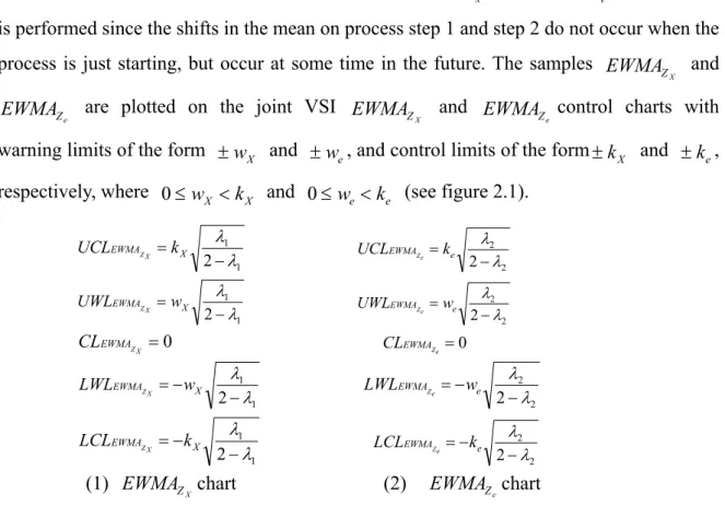
is performed since the shifts in the mean on process step 1 and step 2 do not occur when the process is just starting, but occur at some time in the future. The samples

X

Z

EWMA and

e

Z

EWMA are plotted on the joint VSI EWMA and _ZX EWMA control charts with _Ze

warning limits of the form ±w_X and ±w_e, and control limits of the form±k_X and ± , k_e

respectively, where 0≤w_X <k_X and 0≤w_e<k_e (see figure 2.1). 1 1 2 λ λ − = _X EWMA k UCL Z_X 2 2 2 λ λ − = _e EWMA k UCL Z_e 1 1 2 λ λ − = X EWMA w UWL Z_X 2 2 2 λ λ − = e EWMA w UWL Z_e CLEWMA_ZX =0 =0 e Z EWMA CL 1 1 2 λ λ − − = X EWMA w LWL Z_X 2 2 2 λ λ − − = e EWMA w LWL Z_e 1 1 2 λ λ − − = _X EWMA k LCL X Z 2 2 2 λ λ − − = e EWMA k LCL Z_e

(1) EWMA chart (2)_ZX EWMA chart _Ze

Figure 2.1 The control limits of VSI EWMA_ZX and EWMA control charts_Ze

The search for the special cause 1 and adjustment in the first process step is undertaken when the sample

X

Z

EWMA falls outside the interval (− ,k_x k ), that is when _x

the

X

Z

EWMA chart produces a signal. The search for the special cause 2 and adjustment

in the second process step is undertaken when the sample

e

Z

EWMA falls outside the

interval ( −k_e ,k ), that is when the _e

e

Z

EWMA chart produces a signal. For a

discontinuous process, the two process steps are stopped to search for the special causes and adjustment after at least one signal is obtained from the proposed control charts. The process adjustment is incorrect when the signal is false, but the adjustment is correct when the signal is true and then the process steps are brought back to an in-control state.

The position of the current sample in each control chart constructs the sampling interval of the next sample.

We divide the joint VSI

X

Z

EWMA and

e

Z

EWMA control charts into the following

three regions (2-4). ) , ( 1 X X Z w w I X = − (central region)

(

X X

) (

X X

)

Z -k ,-w w ,k I _X2 = _U (warning region)

(

X X

)

Z -k ,-k I X3 = (control region) (2-4)

VII

(

e e

)

Z -w,w I _e1 = (central region)

(

e e

) (

e e

)

Z -k ,-w w,k I _e2 = _U (warning region)

(

e e

)

Z -k ,-k I _e3 = (control region)

The first region, within two warning limits, is called the central region. The second region, within warning limit and control limit, is called the warning region. The third region, within control limits, is called the control region.

Three VSIs are adopted, 0<t₁<t₂ <t₃<∞. If the samples,

X Z EWMA and e Z EWMA ,

all fall within the central regions,

1 X z I and 1 E Z

I , then the next sampling interval should be long (t ). If one sample falls within the central region but another falls within the ₃

warning region, then the next sampling interval should be median (t₂). If all samples fall within the warning regions, then the next sampling interval should be short (t₁).

The relationship between the next sampling interval (t_m,m=1,2,3) and the position of the current samples is expressed as follows.

, , 1 1 3 if Z I Z I t e i X i Z e Z X ∈ ∈ t if Z I Z I e i X i Z e Z X 2, 1 2 ∈ ∈ (2-5)

t

_m

=

t₂ if Z_Xi∈I_ZX1, Z_ei∈ I_Ze2 t if Z I Z I e i X i Z e Z X 2, 2 1 ∈ ∈

Following Costa (1997), the first sampling interval taken from the process when it is just starting is chosen randomly. When the process is in control, all sampling intervals, including the first one, should have a probability of p of being ₀₁ t , a probability of ₃

03 02 p

p + of being t₂, and a probability of p of being ₀₄ t₁, where 4 1

1 0 =

∑

= i i p , p , ₀₁ 02

VIII ) 1 ) ( 2 )( 1 ) ( 2 ( )) ( 2 ) ( 2 ( ) 1 ) ( 2 ( 0 , 2 2 2 2 2 0 , 2 2 1 ) ( 2 1 ) ( 2 1 ) ( 2 1 ) ( 2 0 , 2 2 0 , 2 2 2 2 2 2 2 2 2 2 2 2 2 1 1 1 1 1 02 2 2 2 2 2 1 1 1 1 1 01 − Φ − Φ Φ − Φ • − Φ = ⎟ ⎟ ⎠ ⎞ ⎜ ⎜ ⎝ ⎛ = − < − < < − − − < < − − • ⎟ ⎟ ⎠ ⎞ ⎜ ⎜ ⎝ ⎛ = − < − < = ⎟⎟ ⎠ ⎞ ⎜⎜ ⎝ ⎛ − Φ − Φ ⎟⎟ ⎠ ⎞ ⎜⎜ ⎝ ⎛ − Φ − Φ = ⎟ ⎟ ⎠ ⎞ ⎜ ⎜ ⎝ ⎛ = − < − < • ⎟ ⎟ ⎠ ⎞ ⎜ ⎜ ⎝ ⎛ = − < − < = e X e e X Z Z Z Z Z e e X X e Ze e Z X Z X Z k k w k w k EWMA k EWMA w or w EWMA k P k EWMA w EWMA P p k w k w k EWMA w EWMA P k EWMA w EWMA P p e e e X X e X X δ λ λ λ λ λ λ λ λ λ λ δ λ λ λ λ δ λ λ λ λ δ λ λ λ λ 　 　 (2-6) ⎟⎟ ⎠ ⎞ ⎜⎜ ⎝ ⎛ − Φ − Φ ⎟⎟ ⎠ ⎞ ⎜⎜ ⎝ ⎛ − Φ Φ − Φ = ⎟ ⎟ ⎠ ⎞ ⎜ ⎜ ⎝ ⎛ = − < − < < − − − < < − − • ⎟ ⎟ ⎠ ⎞ ⎜ ⎜ ⎝ ⎛ = − < − < < − − − < < − − = = − Φ − Φ Φ − Φ • − Φ = ⎟ ⎟ ⎠ ⎞ ⎜ ⎜ ⎝ ⎛ = − < − < • ⎟ ⎟ ⎠ ⎞ ⎜ ⎜ ⎝ ⎛ = − < − < < − − − < < − − = ) 1 ) ( 2 ) ( 2 ) ( 2 1 ) ( 2 ) ( 2 ) ( 2 0 , 2 2 2 2 2 0 , 2 2 2 2 2 ) 1 ) ( 2 )( 1 ) ( 2 ( )) ( 2 ) ( 2 ( ) 1 ) ( 2 ( 0 , 2 2 0 , 2 2 2 2 2 2 2 2 2 2 2 2 2 2 2 2 1 1 1 1 1 1 1 1 1 1 1 04 02 2 2 2 2 2 1 1 1 1 1 1 1 1 1 1 1 03 e e e X X X e Z e Z e e Z e X Z X Z X X Z X e X e e X e Z e Z X Z X Z X X Z X k w k k w k k EWMA k EWMA w or w EWMA k P k EWMA k EWMA w or w EWMA k P p P k k w k w k EWMA w EWMA P k EWMA k EWMA w or w EWMA k P p e e e X X X e e X X X δ λ λ λ λ λ λ λ λ λ λ δ λ λ λ λ λ λ λ λ λ λ δ λ λ λ λ δ λ λ λ λ λ λ λ λ λ λ 　 　 　 　 　 　

To facilitate the computation of the performance measures, w_X , k_X , w and _e k _e

will be specified with the constraint that the probability of a sample falling in the central region is same for both the

X

Z

EWMA andEWMA charts when the process is in control. _Ze

Thus, ) 0 , | | | (| ) 0 , | | | (| _Z < _{X Z} < _X δ₁= ⋅= _{r Z} < _{e Z} < _e δ₂ =

r EWMA w EWMA k P EWMA w EWMA k

P _{X X e e} (2-7)

implying,w_X =w = w ,_e k_X =k =_e k and λ₁=λ₂ =λ.

If both w_X =w =0, and_e t₁=t₂=t =₃ t , then the joint VSI ₀ EWMA and_ZX EWMA charts _Ze

reduce to the joint

X

Z EWMA and

e

Z

EWMA charts with FSIt . ₀

3. COMPARISON OF CONTROL CHARTS

Sampling schemes should be compared under equal conditions; that is, VSI and FSI schemes should demand the same average sampling interval under the in-control period. That is,

[

t |EWMA | k |,EWMA | k, 1 0, 2 0

]

t0

E _{m ZX} < _Ze < δ = δ = = (3-1) Based on the equation (3-1), the following equation can be formulated as

IX ) 0 2 2 ( ) 0 2 2 ( ) 0 ( ) 0 ( ) 0 ( ) 0 ( ) 0 ( ) 0 ( ) 0 ( ) 0 ( 2 1 0 2 1 1 2 1 2 2 1 2 2 1 3 1 , 1 , 2 1 , 2 1 , 1 1 , 2 1 , 2 1 , 1 1 , 1 1 , 1 1 , = − < < − − • = − < < − − • = = ∈ • = ∈ • + = ∈ • = ∈ • + = ∈ • = ∈ • + = ∈ • = ∈ • − − − − − − − − − − δ λ λ λ λ δ λ λ λ λ δ δ δ δ δ δ δ δ k EWMA k P k EWMA k P t I EWMA P I EWMA P t I EWMA P I EWMA P t I EWMA P I EWMA P t I EWMA P I EWMA P t i e i X Ze i e X Z i X e Z i e X Z i X e Z i e X Z i X e Z i e X Z i X Z Z Z Z Z Z Z Z Z Z (3-2) Simplifying,

[

]

[

]

0 )) ( ( 4 ) ( 4 ) 1 ) ( 2 ( ) ( 2 ) ( 2 ) ( 4 2 ) ( 4 2 1 2 3 2 0 1 2 2 3 1 2 3 2 = Φ + Φ − + − Φ − Φ − + Φ + − Φ + + − Φ k t k t t k t k t t k t t w t t t w (3-3) where Φ

( )

⋅ denotes the standard normal cumulative function.

The warning limit is derived as follows:

⎥ ⎥ ⎦ ⎤ ⎢ ⎢ ⎣ ⎡_{− ± −} Φ = − A AC B B w 8 16 16 4 2 1 _(3-4) where

[

2

]

1 2 3 2 0 1 2 2 3 1 2 3 )) ( ( 4 ) ( 4 ) 1 ) ( 2 ( ) ( 2 ) ( 2 2 k t k t t k t C k t t k t t B t t t A Φ − Φ + − − Φ − = Φ − + Φ + − = + − =

However, to obtain w and let 0<w<k , the constraints 0<t₁<t₂ <t₃ < ∞ is required. Thus, the warning limit can be obtained by using equation (3-4) and choosing a combination of the three VSIs, (t₁,t₂,t₃), and the FSI,t . ₀

In this paper, the VSI scheme is compared with the FSI scheme and one adaptive scheme was considered to be better than another when it allows the joint VSI

X

Z

EWMA andEWMA charts to detect changes in the process means on step 1 and step 2 _Ze

faster.

4. PERFORMANCE MEASUREMENT

The speed with which a control chart detects process shifts measures the chart’s statistical efficiency. For a VSI, the detection speed is measured by the average time from either mean shifting until either EWMA or_ZX EWMA chart or both signal, which is known as the _Ze

AATS. That is, the AATS is the mean time that the process remains out of control.

Since T _SCi ~exp(−γ_it), t>0, i=1, 2, the occurrence time, T ,until the first ₍₁₎

special cause occurs is ) exp( ~ _{1 2} ) 1 ( γ +λ T where T₍₁₎ =min(T_SC1,T_SC2) Hence,

X 2 1 1 γ γ + − = ATC AATS (4-1) The average time of the cycle (ATC) is defined as the average time from the start of process until at least one true signal obtained from one or both of the proposed charts and the out-of-control process step1 and/or step2 are correct adjusted. The Markov chain approach is allowed to compute the ATC due to the memory-less property of the exponential distribution. Thus, at each sampling, one of the 32 states is assigned based on whether the process step is in or out of control and the position of samples (see Table 4.1 for the 32 states of the process). The status of the process when the _(i+1)th_{sample is taken,}

and the position of the _{i sample on the joint} th

X

Z EWMA and

e

Z

EWMA charts defines the

transition states of the Markov chain. The joint VSI

X

Z EWMA and

e

Z

EWMA charts produce

a signal when at least one of the samples falls outside its control limits. If the current state is any one of the States 1, 2, 4, 5, 10, 11, 12, 13,17, 18, 20, 21, 24, 25, 27, 28 and 29 then the process steps are not adjusted and the current state may transit to any other state after sampling time interval t , m=1,2,3. If the current state is State 3, it indicates one false _m

signal comes from the second process step then the process is adjusted unnecessarily and State 3 instantly becomes any one of the States 10~13 with probability , j 10~13,and 13 1 10 3 3 =

∑

= = = = j j j P

P . Any one of the States 10~13 thus transits to any one of the States 10, 11, 12, 13 and 32 after a sampling time interval t , with _m

probabilityP_, (t )and

∑

P_, (t )=1, i=10,~13,j=10,11,12,13,32,m=1,2,3.

j ij m

m j

i State 6, 7, 8,

9, 14, 15, 16, 19, 22, 23, 26, 29, 30 and 31 are similar to State 3, since they indicate at least one false signal. .

If the current state is any one of the States 1~31, then there is no true signal, hence States 1~31 are transient states. State 32 is reached when at least one true signal obtained from the out-of-control process step1 and/or step2. State 32 cannot transit to any other state, hence it is an absorbing state.

Denote P be the transition probability matrix, where P is a square matrix of order 32. LetP_i,j(t_m) to be the transition probability from prior state i to the current state j with sampling interval t_m , where t_m is determined by the prior state i,

XI . 3 , 2 , 1 , 32 ,..., 2 , 1 , 32 ,..., 2 , 1 = = = j m

i The transition probability, for example, from state 1 to state 5 with sampling interval t₃ and fixed sample size n is calculated as

( ) ( )

(

)

(

)

2 2 1 3 2 3 1 3 5 , 1 2 ) 0 ( ) 0 ( ) ( ) ( ) ( 3 2 3 1 2 2 w k e e I EWMA P I EWMA P t T P t T P t P t t Z Z SC SC X ZX e Z_e Φ − Φ • • = = ∈ • = ∈ • > • > = − −γ γ δ δ

The calculation of all transition probabilities is shown in Appendix.

From the elementary properties of Markovchains (see, e.g., Cinlar (1975)), the ATC is derived as follows:

(

)

(

)

Mf

(

)

A Tr ATC ₌ ' ₋ −1 ₊ ' ₋ −1 ₊ ' ₋ −1( ) Q I b Q I b t Q I b (4-2) where '₌

(

_p01,_p02,0,_p03,_p04,0,0,0,0,0,0,0,0,0,0,0,0,...,0

)

b is the vector of starting probabilities for

States 1, 2, …, 31, where the first sampling interval has probability p₀₁ (see equation (2-6) for calculation) of being long (or State 1 with probability p₀₁) , the probability p₀₂ + p₀₃

of being median (or State 2 and State 4 with probability p₀₂, p₀₃, respectively) and the probability p₀₄ of being short (or State 5 probability p₀₄); I is the identity matrix of order 31; Q is the transition probability matrix where elements represent the transition probability, P_i,j(t_m) , from transient state I, i=1,…,31, to transient state j, j=1,…,31; M' ( T_f, , T_f T_f T_f T T_f T_f T_f T_f T_f T_f T_f T_f T_f, T_f)

f = 0,0, 00, , , , f,0,0,0,0, , , ,0,0, ,0,0, , ,0,0, ,0,0, ,

is the vector of in-correct adjustment time for State1 ~ State 31;

(

, , *, , , *, *, *, *, , , , , *, *, *, , , *, , , *, *, , , *, , , *, *, *

)

t'= t₃ t₂ t₁ t₂ t₁ t₁ t₂ t₂ t₃ t₃ t₂ t₂ t₁ t₃ t₃ t₂ t₃ t₂ t₃ t₂ t₁ t₃ t₁ t₃ t₂ t₂ t₂ t₁ t₂ t₁ t₁

is the vector of the variable sampling intervals for state1-state 31, where * 1

t is the average time of sampling interval for State 3, 6, 23, 30 and 31, *

2

t is the average time of sampling interval for State 7, 8, 16, 26 and 29, *

3

t is the average time of sampling interval for State 9, 14, 15, 19 and 22. The calculations of *

1

t , *

2

t and * 3

t are shown in Appendix; A is the vector of transition probability, P_i,32(t_m), form transition state i, i=1,…,31, to absorbing state 32; T_ris the time to adjust any process step correctly.

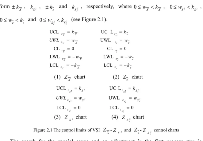
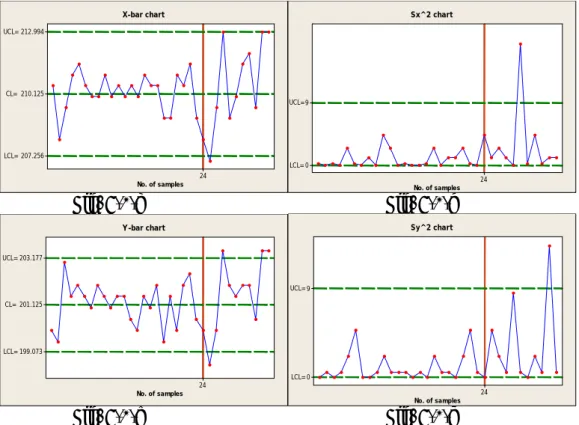
5. AN EXAMPLE

An example of process control for automobile braking system is presented, and the data of the process are measurements of roll weight and bake weight. Let variables X=roll weight

and Y= bake weight be measured from the end of the second process step. The bake weight

produced in the second step is influenced by the roll weight produced in the first step. Two machines are used in the process steps. One machine could only fail in the first process step and shift the mean of X distribution, and another machine could only fail in the second

XII

process step, and shift the mean of Y distribution. Presently, the joint FSI X

Z

EWMA andEWMA_Zecontrol charts are used to monitor the shifts of mean on the two process steps every hour. Information about the state of the process steps is available only through sampling. When the control charts indicate that at least one of the process steps is out of control, it requires adjustment. Sometimes, the process steps may be adjusted unnecessarily when at least one false signal occurs. To construct the control charts, fifty-five samples of size one (X, Y) are taken from Wade and Woodall (1993) to analysis

their statistical relationship. After delete 24 outliers, the QQ plot (see Johnson 1992)of the

31 samples indicates that the data follows bivariate normal distribution. The relationship of quality variables X and Y is expressed by a linear regression model. The fitted model is YˆX =30.3+0.812X (5-1)

Thus, the residuals or specific quality (e) are obtained byY −Y^ X . The estimated means and standard deviations of variables X and e are (μˆ_X =210.5,σˆ_X =1.435), and (μˆ_e=0,σˆ_e =0.817), respectively. That is, when both process steps are in-control,

) 435 . 1 , 5 . 210 ( ~_N 2

X and_e~_N(0,0.8172)_{. From historical data, the estimated failure} frequency is 0.167 time per hour (orγ₁=0.167) for machine 1 and 0.125 time per hour (orγ₂ =0.125) for machine 2. The failure machine1 and 2 are independent and only influence the means of X and Y, but the standard deviations are unaffected. The failure

machine 1 would shift the mean of X to μ^_X+δ₁σ^_X whereδ₁=1.0. The failure machine 2

would shift the mean of e to δ₂σ^_e whereδ₂ =0.5. Hence, for out-of-control process

step1, _X ~_N(210.5₊1.0*1.435,1.4352)_{; for out-of-control step2, e~N(0.5*0.817,0.817}2_). The FSI X Z EWMA and e Z

EWMA charts have control limits placed at ±2.492

andλ=0.05 with average run length 370 (see Montgomery (2005)) when T_f =T_r =0, respectively. The average incorrect adjustment time of any process step is 0.5h (orT_f =0.5) when at least one false signal occurs. The average correct adjustment time of any process step is 6.0h (or T_r =6.0) when at least one true signal occurs. The AATS of the FSI

X

Z

EWMA and

e

Z

EWMA charts is 46.572h. The slowness with which the FSI X Z EWMA and e Z

EWMA control charts detect shifts in the process (δ₁=1.0,δ₂ =0.5) has led the quality manager to propose building the

X

Z EWMA and

e

Z

XIII

VSIs. The construction and application of the proposed VSI EWMA and_ZX EWMA control _Ze

charts is illustrated. The following are the guidelines for using the proposed charts:

Step 1. Let the factor of control limits, k=2.492 and λ=0.05, to maintain the in-control average run length is 370 for each

X

Z EWMA or

e

Z

EWMA control chart.

Step 2. Since 0<t₁<t₂<t <₀ t <₃ ∞ is required, and for performance of process control engineers adopt the combination (t₁=0.09h, t₂=0.1h, and t =3.5 h). ₃

Step 3. Letting t₁=0.09h, t₂=0.1h, t =3.5h , ₃ k =2.492 and λ=0.05 in the equation (3-4) leads to w=0.688.

Consequently, the structures of the proposed VSI

X Z EWMA and e Z EWMA control

charts are as follows.

3990 . 0 = X Z EWMA

UCL UCLEWMAZ_e =0.3990 1102 . 0 = X Z EWMA

UWL UWLEWMAZ_e =0.1102

CLEWMAZ_X =0 CLEWMAZe =0 1102 . 0 − = X Z EWMA LWL LWLEWMAZ_e =−0.1102 3990 . 0 − = X Z EWMA LCL LCLEWMAZ_e =−0.3990 Figure 5.1 the VSI EWMA and_ZX EWMA control limits _Ze

With the design parameters determined, the VSI EWMA and_ZX EWMA control charts _Ze

can be used for controlling the two dependent process steps for producing automobile

braking. According to the VSI scheme, if both samples (

X Z EWMA and e Z EWMA ), fall

within warning limits, then the long sampling interval t =3.5h is taken. If one of the ₃

samples falls within the warning limits but the other falls between warning and control limits, then a middle sampling interval t₂=0.1h is taken. If both samples fall between warning and control limits, then the short sampling interval t₁=0.09h is taken. If at least one sample falls outside the control limits of any proposed control chart, then the process steps are stopped and adjusted. The AATS is used to measure the performance of the proposed VSI control charts. The proposed Markov chain approach is used to obtain the ATC and calculate the AATS. There are 32 possible states, as presented in Table 4.1. The AATS is 38.449h according to equation (4-1).

The VSI scheme improves the sensitivity of the joint FSI EWMA _ZX

andEWMA charts. From the example, in order to detect a shift in the process mean, the _Ze

AATS for the VSI

X

Z EWMA and

e

Z

EWMA charts has been reduced from 46.572 hours to

XIV

An example using the VSIs is introduced now. When the process starts, a random procedure decides the first sampling interval t₂=0.1h with sample of size one, and the observation is (x=213, y=203). The first sample is (x=213, e=-0.3668) and the values of

X

Z and Z are (1.7422, -0.4489). Thus, their _e EWMA_ZX and EWMA values are _Ze

calculated as follows.

(

)

(

1

)

0.05 ( 0.4489) 0.95 0 0.0225 0871 . 0 0 95 . 0 7422 . 1 05 . 0 1 0 , 1 , 1 , 1 0 , 1 − = • + − • = − + = = • + • = − + = e Z e e Z Z X x Z EWMA Z EWMA EWMA Z EWMA X λ λ λ λ

Since both samples fall within the warning limits, the second sample will be observed adopting a sample of size one after long sampling interval t =3.5h. The second sample is ₃

(x=211, y=203). Since Z_X =0.3484 and Z_e =1.5399, soEWMA and_ZX EWMA values _Ze

are calculated as follows.

(

)

(

1

)

0.05 1.5399 0.95 ( 0.0255) 0.0557 1002 . 0 0871 . 0 95 . 0 3484 . 0 05 . 0 1 1 , 2 , 2 , 2 1 , 2 = − • + • = − + = = • + • = − + = e Z e e Z Z X x Z EWMA Z EWMA EWMA Z EWMA X λ λ λ λ

Both samples fall within the warning limits, the third sample will be observed adopting a sample of size one after the long sampling interval t₃ =3.5h. The X Z EWMA and e Z

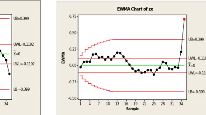
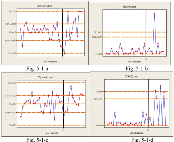
EWMA values for samples 1~35 are illustrated in the Table 5.1, and

plotted on the constructed joint VSIEWMA and_ZX EWMA control charts (Fig. 5.2). We _Ze

find that all EWMA_ZX values fall within the VSI EWMA_ZX chart, but the th

35

e

Z

EWMA value falls outside the VSI

X

Z

EWMA chart. It indicates that the process step1

is in control, butthe process step2 is out of control on the _{35 sample. Hence, the process} th

step2 is stopped and machine 2 is adjusted.

6. PERFORMANCE COMPARISON

BETWEEN ASI AND FSI SCHEMES

Table 6.1 provides the AATS of the VSI and FSI schemes, which are obtained under various combinations of parameters based on orthogonal array (313)

27 L table, 167 . 0 ~ 03 . 0 1= γ , γ₂ =0.06~0.25,δ1=0.5~2.0, δ2 =0.5~2.0, t0 =1.0, 0t3 =1.5~4. , 9 . 0 ~ 1 . 0 2 = t , t₁=0.01~0.09, 0T_f =0.5~3. , T_r =1.0~6.0and n=5. Comparing the AATS between the FSI and VSI

X

Z EWMA and

e

Z

EWMA control charts,

it can be seen that the performance of the VSI

X

Z EWMA and

e

Z

EWMA control charts is

XV

better for detecting small and median shifts in process means ( 0.5≤δ1≤2.0 , 0 . 2 5 . 1 ≤δ₂≤ ). The VSI X Z EWMA and e Z

EWMA control charts save detection time from

3.88% to 30.49% compared to the FSI

X

Z EWMA and

e

Z

EWMA control charts. To examine

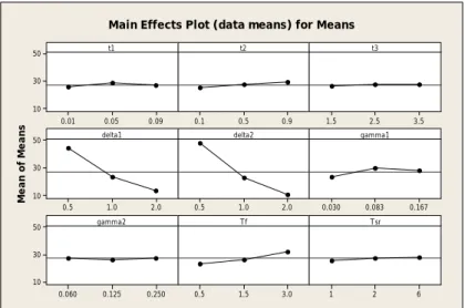
the effects of various parameters on the AATS, the main effects plots show the significant parameters areδ ,1 δ and 2 Tf (see Fig. 6.1). As δ or1 δ increases, AATS decreases; as 2 T f

increases, AATS decreases.

Sometimes, quality engineers cannot

specify the VSIs. The optimal VSIs of the proposed charts are thus suggested. The optimal VSI of the proposed charts are determined using optimization technique (Fortran IMSL BCONF subroutine) to minimum AATS under the same constraints and parameters as described before. The optimum VSI and AATS under various combinations of parameters are illustrated in Table 6.2. We find that the optimum VSI

X Z EWMA and e Z EWMA control

charts save detection time from 4.38% to 34.63% compared to the

FSI EWMA_ZX and EWMA control charts, and the optimum VSI charts _Ze EWMA _ZX

andEWMA control charts also work better than the _Ze EWMA and_ZX EWMA control charts _Ze

with specific variable sampling intervals.

7. CONCLUSIONS

The proposed VSI scheme controlling two dependent process steps with incorrect adjustment substantially improves the performance of the FSI scheme by increasing the speed with which small and median shifts in the means of process steps are detected. We have found that the VSI EWMA and_ZX EWMA control charts always work better (in the _Ze

cases examined) than the FSI EWMA and_ZX EWMA control charts for small and median _Ze

1

δ andδ values. The optimum VSI scheme controlling two dependent process steps with ₂ incorrect adjustment is also suggested when quality engineers cannot specify the VSIs.

This paper considered two dependent process steps with incorrect adjustment. However, a study of the variable sample sizes (VSS), variable sample sizes and sampling intervals (VSSI) or variable parameters (VP)

X

Z EWMA and

e

Z

EWMA control charts under

two dependent process steps with incorrect adjustment is an interesting topic for future research. Other important extensions of the proposed model can also be developed. It is

Insert Table 6.2 Insert Table 6.1 and Figure 6.1

XVI

straight forward to extend the proposed model to study VP control charts or other control charts, such as attribute charts, CUSUM-charts or multivariate charts.

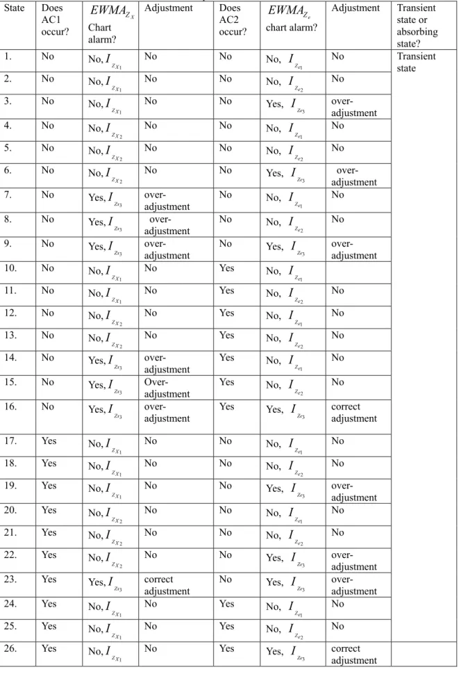
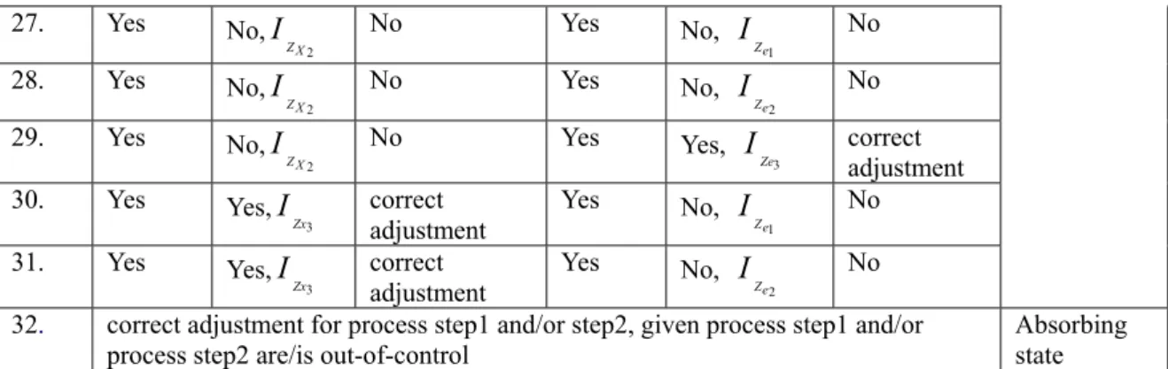
Table 4.1 Definition of 32 process states State Does AC1 occur? X Z EWMA Chart alarm? Adjustment Does AC2 occur? e Z EWMA chart alarm? Adjustment Transient state or absorbing state? 1. No No, 1 X Z I No No _No, 1 e Z I No 2. No No, 1 X Z I No No _No, 2 e Z I No 3. No No, 1 X Z I No No _Yes, 3 Ze I over- adjustment 4. No No, 2 X Z I No No _No, 1 e Z I No 5. No No, 2 X Z I No No _No, 2 e Z I No 6. No No, 2 X Z I No No _Yes, 3 Ze I over- adjustment 7. No Yes, 3 Zx I over- adjustment No _No, 1 e Z I No 8. No Yes, 3 Zx I over- adjustment No No, IZe2 No 9. No Yes, 3 Zx I over- adjustment No Yes, IZe3 over- adjustment 10. No No, 1 X Z I No Yes _No, 1 e Z I 11. No No, 1 X Z I No Yes _No, 2 e Z I No 12. No No, 2 X Z I No Yes _No, 1 e Z I No 13. No No, 2 X Z I No Yes _No, 2 e Z I No 14. No Yes, 3 Zx I over-

adjustment Yes No, IZe1

No 15. No Yes, 3 Zx I Over- adjustment Yes _No, 2 e Z I No 16. No Yes, 3 Zx I over-

adjustment Yes Yes, IZe3

correct adjustment 17. Yes No, 1 X Z I No No _No, 1 e Z I No 18. Yes No, 1 X Z I No No _No, 2 e Z I No 19. Yes No, 1 X Z I No No _Yes, 3 Ze I over- adjustment 20. Yes No, 2 X Z I No No _No, 1 e Z I No 21. Yes No, 2 X Z I No No _No, 2 e Z I No 22. Yes No, 2 X Z I No No _Yes, 3 Ze I over- adjustment 23. Yes Yes, 3 Zx I correct adjustment No Yes, IZe3 over- adjustment 24. Yes No, 1 X Z I No Yes _No, 1 e Z I No 25. Yes No, 1 X Z I No Yes _No, 2 e Z I No Transient state 26. Yes No, 1 X Z I No Yes _Yes, 3 Ze I correct adjustment

XVII 27. Yes No, 2 X Z I No Yes _No, 1 e Z I No 28. Yes No, 2 X Z I No Yes _No, 2 e Z I No 29. Yes No, 2 X Z I No Yes _Yes, 3 Ze I correct adjustment 30. Yes Yes, 3 Zx I correct

adjustment Yes No, IZe1

No 31. Yes Yes,

3

Zx

I correct

adjustment Yes No, IZe2

No 32. correct adjustment for process step1 and/or step2, given process step1 and/or

process step2 are/is out-of-control

Absorbing state

Table 5.1 EWMAZ_X.iand EWMAZ _e.ivalues for the samples 1~35

sample )(_{i x y} e Z_X,i EWMAZ_X.i−1 Z_e,i EWMAZ _e.i−1

1 213 203 -0.3668 1.7422 0.0871 -0.4489 -0.0225 2 211 203 1.2581 0.3484 0.1002 1.5399 0.0557 3 210 201 0.0705 -0.3484 0.0777 0.0863 0.0572 4 210 201 0.0705 -0.3484 0.0564 0.0863 0.0587 5 209 202 1.8830 -1.0453 0.0013 2.3047 0.1710 6 211 202 0.2581 0.3484 0.0187 0.3159 0.1782 7 211 201 -0.7419 0.3484 0.0352 -0.908 0.1239 8 211 202 0.2581 0.3484 0.0509 0.3159 0.1335 9 212 202 -0.5543 1.0453 0.1006 -0.6785 0.0929 10 208 200 0.6954 -1.7422 0.0084 0.8512 0.1308 11 212 202 -0.5543 1.0453 0.0603 -0.6785 0.0903 12 209 201 0.8830 -1.0453 0.0050 1.0807 0.1399 13 210 202 1.0705 -0.3484 -0.0127 1.3103 0.1984 14 210 201 0.0705 -0.3484 -0.0295 0.0863 0.1928 15 211 201 -0.7419 0.3484 -0.0106 -0.9081 0.1377 16 210 200 -0.9295 -0.3484 -0.0275 -1.1377 0.0740 17 210 200 -0.9295 -0.3484 -0.0435 -1.1377 0.0134 18 210 200 -0.9295 -0.3484 -0.0588 -1.1377 -0.0442 19 211 201 -0.7419 0.3484 -0.0384 -0.9081 -0.0874 20 211 202 0.2581 0.3484 -0.0191 0.3159 -0.0672 21 211 201 -0.7419 0.3484 -0.0007 -0.9081 -0.1092 22 210 201 0.0705 -0.3484 -0.0181 0.0863 -0.0995 23 212 203 0.4457 1.0453 0.0351 0.5455 -0.0672 24 209 200 -0.1170 -1.0453 -0.0189 -0.1432 -0.0710 25 209 199 -1.1170 -1.0453 -0.0702 -1.3672 -0.1358 26 210 202 1.0705 -0.3484 -0.0842 1.3103 -0.0635 27 212 203 0.44566 1.0453 -0.0277 0.5455 -0.0331 28 212 204 1.4457 1.0453 0.0260 1.7695 0.0572 29 208 199 -0.3046 -1.7422 -0.0624 -0.3728 0.0356 30 208 198 -1.3046 -1.7422 -0.1464 -1.5968 -0.0462 31 214 204 -0.1792 2.4390 -0.0172 -0.2194 -0.0547 32 212 203 0.4460 1.0453 0.0360 0.5459 -0.0247 33 209 200 -0.1170 -1.0453 -0.0181 -0.1432 -0.0306 34 209 204 3.8830 -1.0453 -0.0695 4.7528 0.2086 35 206 201 8.3200 -3.1359 -0.2228 10.1836 0.7073*

XVIII Sample EW M A 34 31 28 25 22 19 16 13 10 7 4 1 0.4 0.3 0.2 0.1 0.0 -0.1 -0.2 -0.3 -0.4 -0.5 __ X=0 UB=0.399 LB=-0.399 UWL=0.1102 LWL=-0.1102 EWMA Chart of zx Sample EW M A 34 31 28 25 22 19 16 13 10 7 4 1 0.75 0.50 0.25 0.00 -0.25 -0.50 __ X=0 UB=0.399 LB=-0.399 UWL=0.110 LWL=-0.110 EWMA Chart of ze Fig. 5.2 (1) VSI X Z

EWMA control chart Fig. 5.2 (2) VSI

X

Z

EWMA control chart

XIX Me a n o f Me a n s 0.01 0.05 0.09 50 30 10 0.9 0.5 0.1 1.5 2.5 3.5 2.0 1.0 0.5 50 30 10 2.0 1.0 0.5 0.030 0.083 0.167 0.250 0.125 0.060 50 30 10 3.0 1.5 0.5 1 2 6 t1 t2 t3

delta1 delta2 gamma1

gamma2 Tf Tsr

Main Effects Plot (data means) for Means

Fig. 6.1 The main effects for average AATS under various parameters

XX

ACKNOWLEDGMENTS

Support for this research was provided in part by the National Science Council of the Republic of China, grant No. NSC-95-2118-M-004-004.

REFERENCES

[1] Amin, R.W. and Letsinger, W. (1991), “Improved Switching Rules in Control Procedures Using Variable Intervals,” Journal of Quality Technology 25, 36-44.

[2] Capizzi, G. and Masarotto, G. (2003),”An Adaptive Exponentially Weighted Moving Average Control Chart,” Technometrics, 45, 199-207.

[3] Collani, E. Saniga, E. and Weigand, C. (1994),” Economic Adjustment Design for

X Control Charts,” IIE transaction, 26, 37-43.

[4] Cinlar, E. (1975), Introduction to Stochastic Process. Prentice-Hall, Englewood Liffs, NJ.

[5] Deming, W.E.(1982), Quality, Productivity and Competition Position, MIT Press, New York.

XXI

[6] Johnson, R. (1992), Applied Multivariate Statistical Analysis, Prentice-Hall International, Inc., Englewood Cliffs, NJ.

[7] Montgomery, D. (2005), Introduction to Statistical Quality Control, John Wiley and Sons, Inc. USA.

[8] Reynolds, M.R. (1995),” Evaluating Properties of Variable sampling Interval Control Charts,” Sequential Analysis 14, 59-97.

[9] Reynolds, M.R. (1996a),” Shewhart and EWMA Variable sampling Interval Control Charts with Sampling at Fixed Times,” Journal of Quality Technology 28, 199-212. [10] Reynolds, M.R. (1996b),” Variable-sampling-Interval Control Charts with Sampling at

Fixed Times,” IIE Transitions 28, 497-510.

[11] Saccucci, M.S., Amin, R.W. and Lucas, J. M. (1992), “exponentially Weighted Moving Average Control Schemes with Variable Sampling Intervals,” Communication in Statistics---Simulation and Computation 21, 627-657.

[12] Shamma, S.E., Amin, R.W and Shamma, A.K. (1991),” a double EWMA control procedure with variable sampling intervals”, Communications in Statistics-Simulation and Computations, 20, 511-528.

[13] Shewhart, W. (1931), Economic Control of Quality of Manufactured Product. D. Van Nostrand Co., New York.

[14] Tagaras, G. A (1998), “Survey of Recent Developments in the design of Adaptive Control Charts,” Journal of Quality Technology, 30: 212-231.

[15] Wade, M, and Woodall, W. A. (1993),”Review and Analysis of Cause-Selecting Control Charts,” Journal of Quality Technology, 25, No. 3: 161-169.

[16] Woodall, W. (1986),”Weakness of the economic design of control charts, “ Technometrics, 28, 408-409.

[17] Zhang, G. (1984), “A New Type of Control Charts and a Theory of Diagnosis with Control Chats,” World Quality Congress Transactions. American Society for Quality Control, 175-185.

[18] Yang, S. and Yang, C. (2004),”Economic Statistical Process Control for Overadjusted Process Means”, International Journal Quality and Reliability Management, pp. 412-424.

XXII

Appendix: The calculation of all transition probabilities

Notation: 1 ) ( 2 ) ) 2 , 0 ( ~ ( 1 1 =P EWMAZX ∈IZX EWMAZX N − = Φ w − X Z λ λ η ) ( 2 ) ( 2 ) ) 2 , 0 ( ~ ( 2 2 P EWMAZX IZX EWMAZX N k w X Z = ∈ −λ = Φ − Φ λ η ) ( 2 2 ) ) 2 , 0 ( ~ ( 3 3 P EWMAZX IZX EWMAZX N k X Z = ∈ −λ = − Φ λ η 1 ) ( 2 ) ) 2 , 0 ( ~ ( 1 1 =P EWMAZe ∈IZe EWMAZe N − = Φ w − e Z λ λ η ) ( 2 ) ( 2 ) ) 2 , 0 ( ~ ( 2 2 P EWMAZe IZe EWMAZe N k w e Z = ∈ −λ = Φ − Φ λ η ) ( 2 2 ) ) 2 , 0 ( ~ ( 3 3 P EWMAZe IZe EWMAZe N k e Z = ∈ −λ = − Φ λ η )) 2 , 2 ( ~ ( ₁ 1 1 λ λ λ λ δ β − − ∈ =P EWMA I EWMA N X X Z X X Z Z Z = )) 2 , 2 ( ~ 2 ( ₁ λ λ λ λ δ λ λ − − − <w EWMA N EWMA P X X Z Z

XXIII ) 2 2 2 2 2 ( ) 2 2 2 2 2 ( 1 1 1 1 λ λ λ λ δ λ λ λ λ λ λ δ λ λ λ λ δ λ λ λ λ λ λ δ − − − − − < − − − − − − − − < − − − = w EWMA P w EWMA P X X Z Z = Φ(w−δ₁)+Φ(w+δ₁)−1 )) 2 , 2 ( ~ ( ₁ 2 2 λ λ λ λ δ β − − ∈ =P EWMA I EWMA _X N X Z X X Z Z Z )) 2 , 2 ( ~ 2 ( )) 2 , 2 ( ~ 2 ( 1 1 λ λ λ λ δ λ λ λ λ λ λ δ λ λ − − − < − − − − < = N EWMA w EWMA P N EWMA k EWMA P X X X X Z Z Z Z = Φ(k−δ₁)+Φ(k+δ₁)−Φ(w−δ₁)−Φ(w+δ₁) ) ( ) ( 2 1 )) 2 , 2 ( ~ ( 1 1 1 1 1 1 1 2 1 3 3 δ δ β β λ λ λ λ δ β + Φ − − Φ − = − − = − − ∈ = k k N EWMA I EWMA P X X X X Z X x Z Z Z Z Z )) 2 , 2 ( ~ ( ₂ 1 1 λ λ λ λ δ β − − ∈ =P EWMA I EWMA N e e Z e e Z Z Z = )) 2 , 2 ( ~ 2 ( ₂ λ λ λ λ δ λ λ − − − <w EWMA N EWMA P e e Z Z ) 2 2 2 2 2 ( ) 2 2 2 2 2 ( 2 2 2 2 λ λ λ λ δ λ λ λ λ λ λ δ λ λ λ λ δ λ λ λ λ λ λ δ − − − − − < − − − − − − − − < − − − = w EWMA P w EWMA P e Z Ze = Φ(w−δ₂)+Φ(w+δ₂)−1 )) 2 , 2 ( ~ ( ₂ 2 2 λ λ λ λ δ β − − ∈ =P EWMA I EWMA _e N e Z e e Z Z Z )) 2 , 2 ( ~ 2 ( )) 2 , 2 ( ~ 2 ( 2 2 λ λ λ λ δ λ λ λ λ λ λ δ λ λ − − − < − − − − < = N EWMA w EWMA P N EWMA k EWMA P e e e e Z Z Z Z

XXIV =Φ(k−δ₂)+Φ(k+δ₂)−Φ(w−δ₂)−Φ(w+δ₂) ) ( ) ( 2 1 )) 2 , 2 ( ~ ( 2 2 2 2 2 2 2 2 1 3 3 δ δ β β λ λ λ λ δ β + Φ − − Φ − = − − = − − ∈ = k k N EWMA I EWMA P e e e Ze e e Z Z Z Z Z

The transition probability can be expressed by the following general form.

3 , 2 , 1 , 3 , 2 , 1 , 16 ~ 10 for ) 1 ( ) 0 ( ) 0 ( ) ( ) ( ) ( 3 , 2 , 1 , 3 , 2 , 1 , 9 ~ 1 for ) 0 ( ) 0 ( ) ( ) ( ) ( 3 2 3 1 3 2 3 1 2 1 3 2 A 3 1 A 3 , 1 2 1 3 2 A 3 1 A 3 , 1 = = = • • − • = ≠ ∈ • = ∈ • < • > = = = = • • • = = ∈ • = ∈ • > • > = − − − − s r j e e I EWMA P I EWMA P t T P t T P t P s r j e e I EWMA P I EWMA P t T P t T P t P es xr s e Z e r X Z X es xr s e Z e r X Z X z z t t Z Z C C j z z t t Z Z C C j β η δ δ η η δ δ γ γ γ γ 　　　　 　　　　

∑

= − − − − − = = = = • • − • − = ≠ ∈ • ≠ ∈ • < • < = = = = • • • − = = ∈ • ≠ ∈ • > • < = 31 1 3 , 1 3 32 , 1 2 1 3 2 A 3 1 A 3 , 1 2 1 3 2 A 3 1 A 3 , 1 ) ( 1 ) ( 3 , 2 , 1 , 3 , 2 , 1 , 31 ~ 24 for ) 1 ( ) 1 ( ) 0 ( ) 0 ( ) ( ) ( ) ( 3 , 2 , 1 , 3 , 2 , 1 , 23 ~ 17 for ) 1 ( ) 0 ( ) 0 ( ) ( ) ( ) ( 3 2 3 1 3 2 3 1 j j z z t t Z Z C C j z z t t Z Z C C j t P t P s r j e e I EWMA P I EWMA P t T P t T P t P s r j e e I EWMA P I EWMA P t T P t T P t P es xr s e Z e r X Z X es xr s e Z e r X Z X β β δ δ η β δ δ γ γ γ γ 　　　 　　　

∑

= − − − = = = = • • − = ≠ ∈ • ≠ ∈ • < = = = = • • = ≠ ∈ • = ∈ • > = = = 31 1 3 , 10 3 32 , 10 2 1 3 1 A 3 , 10 2 1 3 1 A 3 , 10 3 , 10 ) ( 1 ) ( 3 , 2 , 1 , 3 , 2 , 1 , 31 ~ 24 for ) 1 ( ) 0 ( ) 0 ( ) ( ) ( 3 , 2 , 1 , 3 , 2 , 1 , 16 ~ 10 for ) 0 ( ) 0 ( ) ( ) ( 23 ~ 17 , 9 ~ 1 for 0 ) ( 3 1 3 1 j j z z t Z Z C j z z t Z Z C j j t P t P s r j e I EWMA P I EWMA P t T P t P s r j e I EWMA P I EWMA P t T P t P j t P es xr s e Z e r X Z X es xr s e Z e r X Z X β β δ δ β η δ δ γ γ 　　　　 　　　　

XXV

∑

= − − − = = = = • • − = ≠ ∈ • ≠ ∈ • < = = = = • • = = ∈ • ≠ ∈ • > = = = 31 1 3 , 17 3 32 , 17 2 1 3 2 A 3 , 17 2 1 3 2 A 3 , 17 3 , 17 ) ( 1 ) ( 3 , 2 , 1 , 3 , 2 , 1 , 31 ~ 24 for ) 1 ( ) 0 ( ) 0 ( ) ( ) ( 3 , 2 , 1 , 3 , 2 , 1 , 23 ~ 17 for ) 0 ( ) 0 ( ) ( ) ( 16 ~ 1 for 0 ) ( 3 2 3 2 j j z z t Z Z C j z z t Z Z C j j t P t P s r j e I EWMA P I EWMA P t T P t P s r j e I EWMA P I EWMA P t T P t P j t P es xr s e Z e r X Z X es xr s e Z e r X Z X β β δ δ η β δ δ γ γ 　　　　 　　　　

∑

= − = = = = • = ≠ ∈ ≠ ∈ = = = 31 1 24, 3 3 32 , 24 2 1 3 , 24 3 , 24 ) ( 1 ) ( 3 , 2 , 1 , 3 , 2 , 1 , 31 ~ 24 for ) 0 ( * ) 0 ( ) ( 23 ~ 1 for 0 ) ( j j z z Z Z j j t P t P s r j I EWMA P I EWMA P t P j t P es xr s e Z e r X Z X β β δ δ 　　　　

The transition probabilities for P_2,j(t₂),P_4,j(t₂),P_11,j(t₂),P_12,j(t₂),P_18,j(t₂),P_20,j(t₂),P_25,j(t₂) and P_27,j(t₂) are calculated by replacing t₂ on t for ₃ P_1,j(t₃),P_10,j(t₃),P_17,j(t₃) and

32 ~ 1 ), (₃ , 24 t j= P _j . 32 ~ 1 ), ( ) ( ) ( 32 ~ 1 ), ( ) ( ) ( 32 ~ 1 ), ( ) ( ) ( 32 ~ 1 ), ( ) ( ) ( 2 , 24 2 , 27 2 , 25 2 , 17 2 , 20 2 , 18 2 , 10 2 , 12 2 , 11 2 , 1 2 , 4 2 , 2 = = = = = = = = = = = = j t P t P t P j t P t P t P j t P t P t P j t P t P t P j j j j j j j j j j j j

The transition probabilities for P_5,j(t₁),P_13,j(t₁),P_21,j(t₁) and P_28,j(t₁) are calculated by replacing t₁ on t for ₃ P_1,j(t₃),P_10,j(t₃),P_17,j(t₃) and P_24,j(t₃),j=1~32

32 ~ 1 ), ( ) ( 32 ~ 1 ), ( ) ( 32 ~ 1 ), ( ) ( 32 ~ 1 ), ( ) ( 1 , 24 1 , 28 1 , 17 1 , 21 1 , 10 1 , 13 1 , 1 1 , 5 = = = = = = = = j t P t P j t P t P j t P t P j t P t P j j j j j j j j 1 32 , 0 32 , 32 , 32 = ≠ = P j P _j 31 , 30 , 23 , 6 , 3 , 32 13 12 11 10 , ) ( ) ( ) ( ) ( ) ( 32 , 13 , 12 , 11 , 10 , 31 , 30 , 23 , 6 , 3 , 0 ) ( 1 13 13 2 12 12 2 11 11 3 10 10 * 1 , * 1 , = = + + + = ≠ = = = = = = P t P P t P P t P P t j , , , , i P t P j i t P ,j i ,j i ,j i ,j i j i j i Where 1 13 2 12 2 11 3 10 1* p t p t p t p t t = _i= • + _i= • + _i= • + _i= •