開放式介電泳裝置應用於三維觀測技術

(1)

國立高雄大學土木與環境工程學系

碩士論文

開放式介電泳裝置應用於三維觀測技術

A Three Dimensional Measuring Technology by Appling an

Open-Chip Dielectrohporetic Device

研究生：王世瑋撰

指導教授：施博仁博士

(2)

(3)

I

Nomenclature

 : Permittivity  : Conductivity

 : Ratio of permittivity and conductivity

ˆE : Vector of electric field ˆ

V : Vector of electric potential  : Charge density

 : Electric potential function

, f

 : Angular frequency of electric field

1 2 3

( , , , )

E x x x t : Electric field function

1 2 3

( ,x x x : Symbols of Cartesian coordinate system. They represent , )

( , , )x y z

n

 : Phase angle of electric potential

ˆ

M : Vector of effective dipole moment

r : Radius of particles

 

* K  : Clausius-Mossotti factor c f : Critical frequency ˆ T : Vector of torque , ,

a b c : Length of the semiaxes of an ellipsoid  : Viscosity

(6)

IV  : Angular velocity of the particle

h : Distance between two parallel walls

T xx

f : Coefficient of a particle’s velocity in two parallel walls and infinite fluid

T yx

c : Coefficient of a particle’s angular velocity in two parallel walls and

infinite fluid

l : Length of the microcantilever

 

,

w x t : Deflection of the microcantilever

m

E : Young’s Modulus

 

I x : Momentum of inertia. It is assumed to be constant.

 

m x : Mass per unit length of the microcantilever

d

c : Damping ratio of the microcantilever

 

q x : Interval of applied force

 

p t : Applied force per unit length with time

   

i t g xi

 : Shift - time function associated for time – dependent boundary condition

 

x t,

 : Dynamic deflection caused by the surface homogeneous function

 

n x

 : Orthogonal mode shape function

 

n

T t : Mode time function

,

G Q : Coefficients depend on the boundary condition of the tip-end

n

(7)

V  : 2 d n c m    n n m E I m    2 1 Dn n    , , , n n n n

C D E F : Coefficients depend on the boundary condition at the base-end and tip-end of the microcantilever

,

n n

A B : Coefficients depend on initial condition

 

f

S  t : Amplitude of excitation at frequency  _f

 

F w : Superficial force

Z : Distance between AFM base and the sample R : Radius of the AFM tip

1, 2

A A : Hamaker constant

*

i

k : Slope of the microcantilever

(8)

VI

LIST OF FIGURES

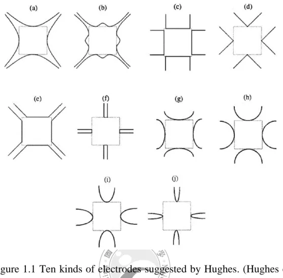
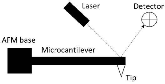
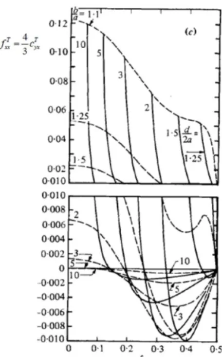
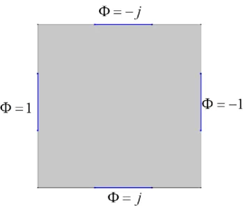
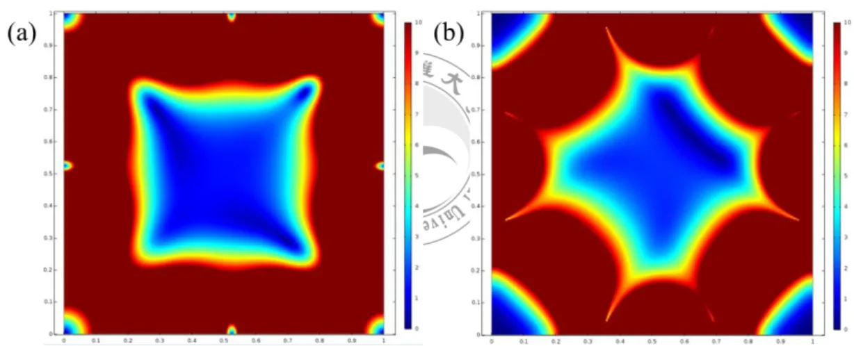
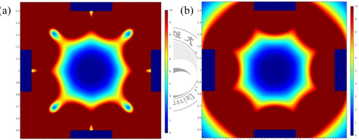
FIGURE 1.1 Ten kinds of electrodes suggested by Hughes. (Hugheset al., 1998). ··· 13 FIGURE 1.2 The basic combination of the AFM contains an AFM base, microcantilever with a tip, a laser, and a detector. ··· 14 FIGURE 1.3 (a) A sketch of Quinke rotation. (b) A sketch of Born-Lertes rotation. ··· 15 FIGURE 2.1 The particle is polarized by the electric field and starts to move to the place where the force is balanced. ··· 33 FIGURE 2.2 An illustrated image of the electrorotation. (Hughes, 2003) 34 FIGURE 2.3 Drag and torque coefficient for a sphere translating between two parallel walls in a fluid at rest (Ganatos et al., 1980) ··· 35 FIGURE 2.4 Schematics of the deflection of AFM microcantilever. ··· 36 FIGURE 3.1 Boundary conditions for the numerical calculation.  is the electric potential. ··· 46 FIGURE 3.2 Distributions of (a) the conventional dielectrophoresis and, (b) the traveling-waved dielectrophoresis. These results were calculated by the numerical method. ··· 47 FIGURE 3.3 (a) The conventional dielectrophoretic force and (b) the traveling waved dielectrophoretic force calculated by the FEM. ··· 47 FIGURE 3.4 The modified configuration for the FEM. ··· 48

(9)

VII

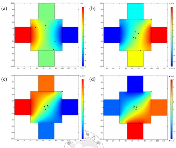
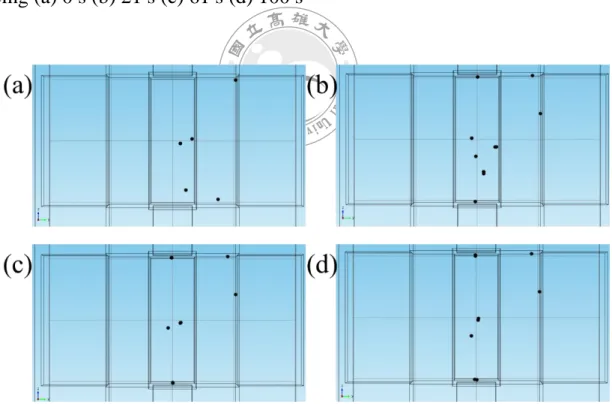
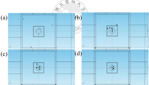
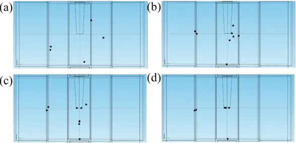
FIGURE 3.5 (a) The conventional dielectrophoretic force and, (b) the traveling-waved dielectrophoretic force calculated by the FEM. ··· 48 FIGURE 3.6 Solution of the particle tracing at (a) 0 (b) 60 (c) 120 (d) 180 second. Blue and red mean -5 Volt and 5 Volt. ··· 49 FIGURE 3.7 Three-dimensional distribution of the dielectrophoretic device. ··· 50 FIGURE 3.8 Simulation result of the three dimensional device. ··· 50 FIGURE 3.9 Modified configuration of the dielectrophoretic device. ···· 51 FIGURE 3.10 Simulation result of the three dimensional deviece. ··· 51 FIGURE 3.11 The three-dimensional simulation at x-y plane of the particle tracing (a) 0 s (b) 21 s (c) 61 s (d) 100 s ··· 52 FIGURE 3.12 The three-dimensional simulation at y-z plane of the particle tracing (a) 0 s (b) 21 s (c) 61 s (d) 100 s ··· 52 FIGURE 3.13 A three-dimensional model with a tip. The bottom of the tip locates at the center of the device. ··· 53 FIGURE 3.14 The result at (a) 0 s, (b) 21 s, (c) 61 s, and (d) 100 s of the simulation with the tip in the x-y plane. ··· 53 FIGURE 3.15 The result at (a) 0 s, (b) 21 s, (c) 61 s, and(d) 100 s of the simulation with the tip in the y-z plane. ··· 54 FIGURE 3.16 The result at (a) 0 s, (b) 5 s, (c) 10 s, (d) 15 s, and (e) 20 s. ··· 55

(10)

VIII

FIGURE 3.17 The result at (a) 0 s, (b) 5 s, (c) 10 s, and (d) 15 s. ··· 55 FIGURE3.18 The total dielectrophoretic force direction at (a) x-y plane, and (b) y-z plane of the three dimensional model based on the real device. ··· 56 FIGURE 4.1 The two experimental electrode setups for (a) rectangular and (b) polynomial electrodes ··· 72 FIGURE 4.2 Spores of Aspergillus Niger. Aspergillus Niger is a spheroid. The radius of the spores is about 4 μm. ··· 73 FIGURE 4.3 The AFM image of the surface of the Aspergillus Niger. The highest position was 0.3 μm. ··· 73 FIGURE 4.4 The mask shows the electrode setup in which R means the rectangular electrodes and P means the polynomial electrodes. ··· 74 FIGURE 4.5 The two-dimensional device with the copper electrodes and observation area. ··· 75 FIGURE 4.6 The two-dimensional device with theplatinum electrodes and observation area. ··· 75 FIGURE 4.7 A two-dimensional electrode device consisting of an eraser and four thin blades. The center distance is 0.1 ~ 0.3 um. ··· 76 FIGURE 4.8 (a) The thin blade before the fabrication. (b) The thin blade after fabrication. (c) The acupuncture needles. ··· 76 FIGURE 4.9 The two-dimensional device with needle electrodes. ··· 77

(11)

IX

FIGURE 4.10 The symmetric condition of the electrodes. The shortest distance between the cross point of the red lines and the midpoint of every electrodes should equal. ··· 77 FIGURE 4.11 The controller, NI USB-6343, made by National Instrument.

··· 78 FIGURE 4.12 The wave diagram measuring by the oscilloscope at (a) 10 kHz, (b) 20 kHz, and (c) 30 kHz. ··· 79 FIGURE 4.13 The rotation sequence of the Labview. (a) Front panel. (b) Block diagram. Block (1) to (4) represent the electrodes with the phases 0⁰, 90⁰, 180⁰ and, 270⁰. ··· 80 FIGURE 4.14 Front panel of the separated parameters program. The block (1) to (4) mean the amplitude and frequency exert to the electrode with phase 0⁰, 90⁰, 180⁰ and, 270⁰. ··· 81 FIGURE 4.15 Block diagram of the separated parameters program. (1) The switch. (2) The input parameters. (3) Signal settings. (4) The output setting. ··· 82 FIGURE 4.16 The block diagram of the rectangular shifting program. (1) The time counter. (2) Here are 8 intervals of time. ··· 83 FIGURE 4.17 Arrangement of the experiment. (a) An optical microscope with a CCD records the image of the particle’s motion. (b) The signal generator is connected to the dielectrophoretic device.··· 84

(12)

X

FIGURE 4.18 The rotational test result at (a) 0 s, (b) 1 s, (c) 2 s, (d) 3 s, (e) 4 s, and (f) 4.23 s at certain frequency, 20 kHz. The red and blue arrows are the positions at the start and the end of the second.··· 85 FIGURE 4.19 Rotational test result at (a) 0 s (b) 1 s (c) 2 s (d) 3 s (e) 3.25 s.

The red and blue arrows are the positions at the start and the end of the second. ··· 86 FIGURE 4.20 Angular velocity – frequency diagram of material Cu and Pt.

··· 87 FIGURE 4.21 -Im K_ *

 



_ - Angular Velocity diagram. ··· 87 FIGURE 4.22 - - Frequency diagram where the frequency range is from 15 kHz to 35 kHz. ··· 88 FIGURE 4.23 The rotation test resulting with needle electrodes at (a) 0 s, (b) 1 s, (c) 2 s, (d) 3 s, (d) 3.875 s. ··· 89 FIGURE 4.24 A designed path for the shift test. When t = (a) 0 ~ 20 s, (b) 21 ~ 30 s, (c) 31 ~ 40 s, (d) 41 ~ 60 s, (e) 61 ~ 80 s, (f) 81~ 100 s, (g) 101 ~ 110 s, and (i) 111 ~ 120 s. ··· 90 FIGURE 4.25 The path of the particle in shifting test. The particle starts from 20 s and ends at 120 s. ··· 91 FIGURE 4.26 The result of amplitude difference is 2 V at (a) 0 s, (b) 20 s, (c) 30 s, (d) 40 s, (e) 60 s, (f) 80 s, (g) 100 s, (h) 110 s, and (i) 120 s. ··· 92

 

*

(13)

XI

LIST OF TABLES

TABLE 3.1 The parameters of the RBC and of the fluidic medium. ...55 TABLE 3.2 The parameters of the silicon. ... 56 TABLE 3.3 The modified parameters of Aspergillus Niger and fluidic medium. ... 56

(14)

1

開放式介電泳裝置應用於三維觀測技術

指導教授：施博仁博士國立高雄大學土木與環境工程所學生：王世瑋國立高雄大學土木與環境工程所摘要本論文研製之二維介電泳裝置可操縱微小粒子，並以黴菌孢子作為實驗的範例。此裝置與前人所開發之封閉式的裝置不同，本論文利用開放式之介電泳裝置，使細胞檢測之三維觀測技術能有更多的選擇。此外，本文以實驗及理論分析得知微小粒子之轉動與平移速度，故在操縱的過程中可依據理論所得之參數進行實驗的設置。文中基於電場理論，配合電極位置配置的邊界條件，推導二維的介電泳力、行波介電泳力及介電力矩等場值。針對二維的理論場形分佈，也利用 Comsol 套裝軟體的計算技術建立二維模型，藉此建立模擬相關場形的半數值分析技術。透過理論場形和半數值場形的比對，確認半數值模擬技術的可靠性後，將技術擴充到三維的分析，和任意的邊界電極分佈，並分析掃描探針對於系統之影響。本論文亦討論了以不同的製程方法製造介電泳裝置，並且進行實驗測試，此測試證明除了一般半導體製程可進行介電泳裝置之製作外，尚有其他較低成本的製程方法製作介電泳裝置。首先，本論文設計一以行波介電泳為基礎的三維位移裝置，對標的物進行三維平移和旋轉等動作。藉旋轉標的物的技術，並配合可在液體中掃描觀測的原子力顯微鏡，實踐三維原子力顯微鏡掃描術。接著進行實驗以行波介電泳之位移裝置操控黑曲黴孢子。在實驗中，我們以開放式之空間進行介電泳實驗，從實驗可以求得在特定之交流電頻率下黑曲黴的轉速與移動速度。藉由將實驗數據帶入介電泳理論中即可得到完整的 Clausius-Mossotti 常數，輔以理論可得粒子之速度，增進粒子操縱術之精度。另外，本論文亦進行了三維介電泳裝置之設計與製作及原子力顯微鏡探針之影響探討。關鍵字：行波介電泳、開放式介電泳裝置、原子力顯微鏡、黑麴黴

(15)

2

A Three-Dimensional Measuring Technology by Applying

an Open-Chip Dielectrophoretic Device

Advisor: Dr. Po-Jen Shih

Institute of Civil and Environmental Engineering National University of Kaohsiung

Student: Shih-Wei Wang

Institute of Civil and Environmental Engineering National University of Kaohsiung

ABSTRACT

The purpose of this thesis is developing a three-dimensional device. This device can execute the three-dimensional manipulation of a small specimen; for example: Aspergillus Niger. The device is different from other devices, and it is designed by basing on an open-chip device. This difference provides much opportunity to the microscope to realize the three-dimensional scanning. In this paper, we apply the dielectrophoretic theory to calculate the two-dimensional forces as a semi-numerical model, and then a finite element method (FEM) software was applied to simulate this model and to provide the further comparsion. By comparison of the results between the theory model and the FEM model, the reliability and accuracy of the semi-numerical method were confirmed. Accordingly, the analysis of arbitrary electrode distribution and the affection from an AFM tip were studied to develop a three-dimensional model. In this thesis, we provide three different methods for manufacturing the dieletrophoretic device. The first method is a traditional method by applying MEMs processing; the second method is hand-made by combining a soft substrate and a thin blade; and the third method is an improvement from the second method by replacing the thin blade with the acupuncture needles to improve the symmetricity of electodes. As the experimental setup, it measured the translational and rotational velocity at the specific frequency of the Aspergillus Niger. Then we substituted the velocity into the dielectrophoretic formula, and the Clausius-Mossotti factor could be evaluated.

Keywords: Traveling-wave dielectrophoresis, open-chip device, dielectrophoretic device,

(16)

3

Chapter 1 Introduction

1.1 Background

In order to control particles moving, there are many methods forcing on manipulating particles. In addition, when it comes to a biological cell, the non-contact forces, such as the best choose, are required to avoid the physical contacting to ruin the cell. Accordingly, there are the ultrasonic, optical, hydrodynamic, and electromagnetic forces. The optical method is performed by optical beam; the hydrodynamic force is operated through the whirling flow; and the electromagnetic forces can be separated into electric method and magnetic method. However, there are disadvantages among these different kinds of forces from methods, such as that the force of the optical beam is too small to trigger or to move a big specimen while whose diameter is greater than 100 μm (Takeshi Hayakawa, et al., 2015).

In addition, the dielectrophoresis is chosen as the applying force in our study. The dielectrophoresis has become an important method of manipulating a particle especially in the field of controlling the biological particles (Benhal, 2013; Jones, 2003). In this method, the dielectrophoresis can operate a particle in a fluidic environment, and the particle is in the ideal medium, liquid, which helps particle float and frictionless. Moreover, the dielectrophoresis method can be applied in fields of isolating particles, separating DNA, traping particles at a specific location, etc. However,

(17)

4

according to references, these applications of the dielectrophoresis are limited in the two-dimensional motion in horizontal plane until now. In this paper, we try to develop a device which can operate a particle moving in three-dimensional space.

The dielectrophoresis were firstly found by Phol (Phol, 1978). Wang et al. calculated the amplitude and the phase in the operation system, and they also analyzed torques and forces on particles in an electric field with special concept (Wang et al., 1994). They consider the time averaged design in which the time averaged concept is defined by

 

1 t t



 



t f t f t t d t t t       



(1.1)

Where t is time, and t is a small interval of time. The detail calculation is shown in the appendix. In addition, they pointed out that the torque is strongly associative with the phase difference between the x-axis and the y-axis. In 1998, Hughes and Morgan studied the two-dimensional and time-depended electric field, and they pointed out two important results (Hughes and Morgan, 1998): Firstly, a device which accomplishes both translation and rotation could be designed through an ideal configuration of the electrodes. Secondly, there are ten different distributions of the electrodes suggested to control the particles. In Figure 1.1, (a) ~ (j) represent

(18)

5

polynomial, bone, square, pointed pyramidal, truncated pyramidal, pin, oblate ellipse, circular, prolate ellipse, and narrow prolate ellipse electrodes.

In addition to the dielectrophoresis, the total dielectrophoretic force including conventional dielectrophoretic force and traveling-waved dielectrophoretic force were introduced, and they applied both forces and torques on the target subject without the device contacting the subject directly. And so that it could be widely used in biological particles and cells (Benhal, 2013; Jones, 2003). In the total dielectrophoretic mode, when a dielectric particle experiences a non-uniform electric field, the dielectrophoretic force is greater than the initial inertial force. Afterward, the particles starts to move under the electric pathes. Here this phenomenon is called dielectrophoresis (Jones, 2003). That applying an AC electric to the electrodes makes a particle stably translate and rotate in the electric field is so called the traveling-waved dielectrophoresisp (Chen, 2008; Jones and Washizu, 1996).

When it is setup that a constant magnitude and frequency to every electrode and AC voltage are given and a 90 phase shifts between each nearby electrode, this rotating electric field gives the particle a specific torque. This model is called by the electrorotaion. When the electric field is not parallel to the dipole, it becomes a torque. This is named by the electroorientation. The above two methods, the electrorotation and the

(19)

6

electrooientation, are based on the same theory; and both of these dielectrophoretic forces are called dielectrophoresis.

In recent years, researchers have scanned many surfaces of the materials, and these results have reached to the sub-nano scale. Among these materials, the biological cells have not been mentioned for many times. There are some difficulties when performing a three-dimensional scan on the biological particles, including the medium and environment. In this case the particles need a normal saline to avoid the particle being destroyed. The most common way to scan a particle’s surface is using the Scanning Tunneling Microscope (STM) which is operating in vacuum. Once the particle is a biological cell, the particle should be coated with other material to avoid the cell exploding in the vacuum environment. Coating a thing is as soft as the biological cell may make the cell deform. Or the coating material is bonded with each other. Those make the depth of the surface become shallow, and hence the result is unreal.

There are three different kinds of the microscope, such as Atomic Force Microscope (AFM), Transmission Electron Microscope (TEM), and STM, can image micro-scalar particles or even nano-scalar particles. A STM requires a conductive specimen for scanning. A TEM requires a vacuum environment to execute the scanning. Because of the ability of performing a scan in the normal condition and in the water, the AFM is become a popular

(20)

7

equipment. An AFM is a microscope which can execute the nano-scale scanning with piezoelectric components in the open air or in the open liquid environment, and it was widely applied in measuring the contour of biological specimen (Shih and Shih, 2015). The AFM contains a laser, a detector, a vibration base, and a microcantilever with a tip. The major mechanism can assemble as Figure 1.2. An AFM base is a piezoelectric vibrating base. A microcantilever is fixed on the AFM base, and a tip locates at the free end of the microcantilever. When a laser hits the back of the microcantilever, the laser deflects to the detector. While the detector receives the signal, it transmits the signal to the computer which runs the further calculations.

Operating methods of the AFM can generally be separated into two modes. One is the contact mode, and the other one is the dynamic mode. Static mode is a mode of a static force, and this mode operates slowly to move down and to contact the sample. When the tip is barely a few nanometers to touch or contact the specimen, the tip is dragged down by the van der Waals' force. The advantage of the contact mode is that it directly touched the sample. The distortion of the particle’s image would be less than non-contact mode. This advantage is more obvious when the specimen is rigid. The responsive signal of the contact mode is proportional to the

(21)

8

displacement of the tip and noise. The disadvantage is that the tip can directly touch the specimen if the cantilever is with high stiffness. This will make the specimen be destroyed. On the other hand, the dynamic mode can also be separated into many details. Generally, the dynamic mode is a way that vibrating the cantilever and the tip moves toward the specimen. It is generally called the tapping mode (TM). And it uses a piezoelectric material to make the microcantilever do a simple harmonic motion. While the tip approaches the sample, the amplitude of vibration becomes small and the natural frequency shifts high. The method measuring the amplitude is also called the amplitude mode (AM). The method detecting the change of the vibrating frequency is also called the frequency mode (FM). To avoid the directly physical contact specimen during the process, the dynamic mode will be chosen when it scans biological specimen.

1.2 Literatures Survey

For measurement of small particles, there are few methods to control and image the micro or nano-particles. The dielectrophoresis was chosen to be our control method, and the AFM which can scan the contour of a particle in the liquid is chosen as the image method in this thesis. A closed chamber is needed when the dielectrophoresis is applied to perform a three-dimensional manipulation. But this closed chamber makes observation by using the AFM

(22)

9

become a difficult problem. This paper will present a viable open-chip device for the three-dimensional motion which is controlled by the dielectrophoretic force. A successful dielectrophoretic device had to complete three dimensional manipulations on the particle, and it should be trapped the particle at the center area.

The dielectrophoresis was first introduced by Phol (Phol, 1978). The further calculation was completed by Wang (Wang et al., 1994). He proposed a time averaged force calculation to unify the dielectrophoretic forces. These results made the calculation of the dielectrophoretic forces become easier. Jones and Washizu followed Wang’s concept to complete the multipolar questions about the dielectrophoretic forces. The electrorotation was also mentioned in Jones and Washizu’s studies (Jones and Washizu, 1996; Washizu and Jones, 1996). In 2003, Jones proposed a method to calculate the dieletrophoretic force on a biological specimen which was in the liquid environmental and experienced a non-uniform electric field (Jones, 2003). Accordingly, there are two kinds of the particle rotation: the Quincke rotation and the Born-Lertes rotation which is also called electrorotation (see Figure 1.3). In Figure 1.3, (a) is a sketch of Quinke rotation, where ₁ and ₂ are the conductivity of the medium and particle; ₁　 and ₂ are the permittivity of the medium, and the particle,   ₁  ₁ ₁ and ₂  ₂ ₂. The quince rotation happens when ₂ ₁. (b) is a sketch of Born-Lertes rotation. It

(23)

10

happens when the electrodes are applied a current with the phase difference 90⁰.

The method in this thesis is mainly used by the electrorotation for the rotation and translation of a particle. Hölzel introduced a method for the calculation of the two- and three-dimensional distribution of the electric field in the arbitrary configuration of the electrodes. For any voltages, phase, and frequency being applied in the electrodes, this method can determine the distribution of the electric field (Hölzel, 1993). Hughes et al. also calculated the amplitude and the phase of an AC electric field, and the concept of the time average was applied in their study. Their results pointed out that the torque was related to the difference of the phase between the x- and y- components. The square of the electric field magnitudes also had the contribution for the electrorotation (Hughes et al., 1994). Hughes et al. measured the spatial dependence of the rotation rate for a polynomial electrode array. They showed that the torque could vary in excess 50% for different position within this chamber (Hughes et al., 1999).

A widely adopted method for investigating the hydrodynamics caused by a vibrating probe in liquid is the boundary integral formulation, which is a semi-analytical method with a strongly theoretical background. Tuck (1969) proposed an integral method which has subsequently been applied to practical applications such as AFM and microelectromechanical systems. The tapping

(24)

11

mode has become a widely used technique for scanning bio-specimens (Tuck, 1969). In tapping mode of the AFM, when a tip taps the specimen, the system suffers interference from liquid in the small gap between the beam and the specimen. Meanwhile, both the beam and the tip apply pressure to the liquid, and this pressure works on the specimen. Möller et al. (1999) found that averaged heights of a topography of outer hexagonally packed intermediate (HPI) layer surfaces and extracellular cytoplasmic purple membrane surfaces measured by the tapping mode were up to 25% smaller than those measured by the contact mode (Möller et al., 1999).

1.3 Objective of this Thesis

An AFM can execute a scanning in normal temperature and pressure (NTP) condition or in a liquid environment. In the biological techniques, building a device that can use single process to complete a 3D imaging is not an easy task. We will develop an open-chip dielectrophoretic device and the procedures of manufacturing in this thesis. The open-chip dielectrophoretic device will be introduced in following chapters. The procedure mainly contained three parts. First, the theoretical analysis was introduced and built a two dimensional model for dielectrophoresis. Second, the simulation of the particle’s motion was done by finite element method. Third, the experiments

(25)

12

were done by applying devices which were manufactured by different methods.

(26)

13

Figure 1.1 Ten kinds of electrodes suggested by Hughes. (Hughes et al., 1998).

(27)

14

Figure 1.2 The basic combination of the AFM contains an AFM base, microcantilever with a tip, a laser, and a detector.

(28)

15

Figure 1.3 (a) A sketch of Quinke rotation. (b) A sketch of Born-Lertes rotation.

(29)

16

Chapter 2 Theory of Dielectrophoresis

The theory of dielectrophoresis introduces the dielectrophoresis from the electrostatics, through the conventional dielectrophoresis and the traveling-waved dielectrophoresis, to the fluidic force. The dielectrophoresis is a force induced by the effective dipole of the particle, and the electric dipole can be expressed by the electric potential. Those mean the dielectrophoretic force can be written as function of the electric potentials. The particle needs to suspend in the liquid to achieve the manipulation, and so the fluidic force is also an important issue to suspend the particle.

Through solving the theoretical solution, we can set up a numerical model. Then we could set up a correct FEM model for analyzing the dielectrophoretic problem by comparing the numerical model and FEM model. By building a FEM model, the dieletrophoretic problem could be analyzed with much less time.

2.1 The dielectrophoresis theory and the general solutions

2.1.1 Electrostatics

(30)

17

presented by the gradient of the electric potential, Vˆ, i.e.

ˆ ˆ

E V (2.1)

By substituting the governing equation of the electrostatics into Eq. (2.1), we can obtain the formula,

2_Vˆ 





  (2.2)

where  denotes the charge density, and  denotes the permittivity of the medium. Eq. (2.2) is known as the Poisson’s equation for the electric potential. When it is assumed the charge density is zero, this equation can be reduced to the Laplace’s equation as

2_Vˆ ₀

  (2.3)

The electric potential for an AC electric field with an angular frequency , can be shown as





( , , , ) Re ( , , ) j t

V x y z t   x y z e  (2.4) where the electric potential, , can be separated into two terms and can be written as,

( , , )x y z _ _r( , , )x y z j _i( , , )x y z _

     (2.5)

where j  1. Accordingly to the basic theory of the electrostatics, both terms,_r( , , )x y z and _i( , , )x y z , have to satisfy the Laplace equation,

(31)

18 2 ₀ r   (2.6) and 2 0 i   . (2.7)

2.1.2 General solutions to the dielectrophoresis

Generally speaking, the general theory of the dielectrophoresis consists the traditional dielectrophoresis (the conventional dielectrophoresis) and the traveling-waved dielectrophoresis. The general dielectrophoresis is the convenient and the noncontact force to manipulate particles. It may be a novel technique for manipulating the biological cells or bio-particles. Here the traditional dielectrophoresis is one of the general dielectrophoresis and is a phenomenon of the particle experiencing a non-uniform electric field. Whether the particle is charged or not, the particle will be effected by the dielectrophoresis. Once the particle is effected, the particle will be polarized. After the polarization, the particle will start to move according to the shape of the electric field, as shown in Figure 2.1. Here the force of the dielectrophoresis is strongly affected by the arrangement of the electrodes, and different configuration of the electrodes may induce a maximum 50% difference of the dielectrophoresis. For a quasi-static condition, the electric

(32)

19 field can be expressed like,

3 1 2 3 1 2 3 1 2 3 1 ˆ ( , , , ) ( , , )cos( ( , , )) n x n n n E x x x t E x x x  t  x x x x  



  (2.8)

where ( , , )x x x denote the coordinate system by ₁ ₂ ₃ ( , , )x y z , (E_x₁,E_x₂,E_x₃) are the amplitudes of electric field, ( , , )  ₁ ₂ ₃ are the phase components, t

is time,  is the angular frequency, and ( , , )x x x are the unit vector of ˆ ˆ ˆ₁ ₂ ₃

1 2 3

( , , )x x x in the Cartesian coordinate. Wang et al. (X-B Wang et al., 1994)

had pointed out the time-averaged general solution of the dielectrophoresis by effective moment method,

1 2 3

ˆ_{( ,} _, _{, )} ₍ ˆ ₎ˆ

F x x x t  M E (2.9)

where the effective dipole moment, ˆm, of a spherical particle with radius, r, and the center of the particle locate at ( , , )x x x can be presented by ₁ ₂ ₃



 



3 3 * 1 2 3 1 * ˆ ( , , , ) 4 Re ( ) cos( ) ˆ Im sin( ) m xn n n n n M x x x t r E K t K t x                      



(2.10)

So Eq. (2.9) can be written as,

 

3 3 * 2 1 2 3 1 3 * 2 1 1 ˆ ( , , , ) 2 Re 2 ˆ Im n n m x n x n n n F x x x t r K E K E x        _ _  _ _{ }   _ _ _ _       _  _{ } _     _  _    



(2.11)

(33)

20 where *

 

Re K_  _ and *

 

Im K_  _ are the real and imaginary part of complex Clausius-Mossotti factor. It is defined by

 

* * * * ₂ * p m p m K         (2.12) which * ( ) p p p j     and * ( ) m m m j

    . m and p are the

permittivity of the surrounding medium and the particle. m and p are the

conductivity of the surrounding medium and the particle. We choose the sphere and oblate spheroid as two models in normal saline, and it obtains p

and p by the model proposed by Gimsa (Gimsa et al., 1996):

0 2 0.162 50 1 p c f f                _ _   _ _       (2.13) and 2 2 0.135 0.4 1 c p c f f f f                     (2.14)

where f is the frequency, fc =15 MHz, m= 78.5 0, and m 1.327 S/m.

An illustrate image of the electrorotation is shown as Figure 2.2. The electrorotation is also initiated by one of the dielectrophoretic forces, torque.

(34)

21

Torque Tˆ can be calculated by using the effective moment approach (Jones,

1995),

1 2 3

ˆ_{( ,} _, _{, )} ˆ ˆ

T x x x t ME (2.15)

where ( , , )x x x is the axis which the torque act on the center axis of the ₁ ₂ ₃

particle. By applying Eqs. (2.2), (2.10), and (2.15), we determine the torque

ˆ T as,

 

















3 * 1 2 3 2 3 2 3 1 3 1 3 1 2 1 2 1 2 3 ˆ_{( ,} _{, , )} ₄ _Im _sin _ˆ ˆ ˆ sin sin m x x x x x x x x x x T x x x t r K E E x E E x E E x                    (2.16)

Force expressed in Eqs. (2.11) and (2.15) can be rewritten as the followed equations,

 

2 2 3 3 3 * 1 2 3 1 1 2 3 2 * 1 1 ˆ ( , , , ) 2 Re 2 + Im i r m n l l n n i r r i n l n n l n n F x x x t r K x x x K x x x x x x        _ _ __      _ _ _ _ __      _ _ _ __ _ _ _ __    _ _    __       _ _   _ _            _         



xˆ_l  (2.17) and

 

3 * 1 2 3 1 2 3 3 2 2 3 3 1 1 3 1 2 2 1 ˆ_{( ,} _, _{, )} ₄ _Im _ˆ ˆ ˆ i r i r m i r i r i r i r T x x x t r K x x x x x x x x x x x x x x x    _{ }_ _   _ _      _{ }   _  _   _ _ _   _                               (2.18)

(35)

22

Equations (2.17) and (2.18) are more suitable for numerical method, because the sine function is a difficult part for the numerical calculation. An expression of the electric potential like Eq. (2.17) and (2.18) can avoid the calculation of the sine function term in Eq. (2.16). This characteristic makes the electric potential expression a better function for the numerical calculations.

The above equations are based on the spherical particle, but the actual shape of the erythrocyte is much like an ellipsoid. This kind of shape can calculated by the Eqs. (2.17) and (2.18). The ellipsoid has three semiaxes, a, b and c, and so the equations should be written as (Yang and Lei, 2007),

 

2 2 3 3 * 1 2 3 1 1 2 3 2 * 1 1 ˆ ( , , , ) 2 Re 2 + Im i r m n l l n n i r r i n l n n l n n F x x x t abc K x x x K x x x x x x         _ _ __      _ _  __ _ _ _ _  _ _ _ __ _ _ _ __    _ _    __       _ _   _ _            _         



xˆ_l  (2.19) and





1 2 3 1 1 2 2 3 3 ˆ_{( ,} _, _{, )} ₂ ˆ_ˆ ˆ _ˆ ˆ _ˆ m T x x x t   abc T x T x T x (2.20) where

(36)

23

 





 





* * 1 2 3 2 3 3 2 * * 2 3 2 3 3 2 ˆ _Im _Im Re Re i r i r i r i r T K K x x x x K K x x x x          _{ } _     _ _      _{ } _     _ _                       (2.21)

 





 





* * 2 3 1 3 1 1 3 * * 3 1 3 1 1 3 ˆ _Im _Im Re Re i r i r i r i r T K K x x x x K K x x x x          _{ } _     _ _      _{ } _     _ _                       (2.22) and

 





 





* * 3 1 2 1 2 2 1 * * 1 2 1 2 2 1 ˆ _Im _Im Re Re i r i r i r i r T K K x x x x K K x x x x          _{ } _     _ _      _{ } _     _ _                       (2.23)

2.2 Viscous force and torque applying on the particle

Following these assumptions: (1) low Reynolds number flow, (2) rigid spherical particle, (3) dilute volume concentration of particles in suspension, and (4) laminar flow, a spherical particle with radius r is modified to moves in an infinite fluid with viscosity



where derived by Stokes (1851) and Kirchhoff (Lamb, 1932), respectively, as,

F = 6_  rU (2.24) and

3

8

(37)

24

where U and  are the linear and angular velocity of the particle relative to fluid at the center of the sphere. Ganatos et al. (1980) studied the problem between two parallel walls by applying collocation theory, and they found the forces 1 1 F= 6 T xx U r h rf  _  _    (2.26) and 2 1 1 8 T yx c r h T_ r _  _      (2.27) where f_xxT and T 1 yx c h    

  are as shown in Figure 2.3.

2.3 Vibration theory of an atomic force microscope

Dynamic AFM has been widely used in high resolution images on a nanometer scale for decades. The most commonly used operating mode of dynamic AFM involves a feedback system of amplitude modulation and exploits the fact that the tip of the microcantilever oscillates with amplitudes of a few tens of nanometers. An interaction between tip and sample induces a strong nonlinearity in the motion of the tip; such nonlinearity includes tip-jump, bistability (Lee et al., 2002; Samtos et al., 2010), snapping, hysteresis, intermittency (Jamitzky and Stark, 2010), period doubling, and

(38)

25

bifurcation from periodic to chaotic oscillations (Hu and Raman, 2006). These nonlinearities reduce the accuracy of the AFM. Shih (Shih, 2012) provided an easy method to understand the mechanism of the tip-jump. He also proposed that the tip-jump is a predictable motion, and the tip-jump always happens before the tip touched the sample.

2.3.1. Equations of the AFM tip motion

The elastic Bernoulli-Euler equation of the microcantilever motion is that

 

2

 

2

 

   

2 2 2 2 , , , m d w x t w x t w x t E I x m x c q x p t x x x x       _ _ _    _  _   (2.28)

Where w(x,t) is the deflection; Em is Young’s modulus of the cantilever; I(x)

is the moment of inertia and is assumed to be constant; m(x) is the mass per unit length with the microcantilever assumed to be homogeneous; c is the damping coefficient, and q(x)p(t) represents the applied force per unit length on the microcantilever. Figure 2.4 is schematics of the deflection of AFM microcantilever. Δ1(t) is the elevated height of AFM base, Δ2(t) is static

deflection caused by the force at the tip end, and ξ(l, t) is the dynamic deflection caused by the surface homogeneous wave. The deflection of the cantilever can be written as,

 

2

   

1 , , _i _i i w x t  x t t g x   



 (2.29)

(39)

26  

_{   }

2   1 IV IV m d m i i i i i i i E I m c  q x p t E I g m g c g       



_      _ (2.30)

The deflection ξ(x,t) can be obtained under a constant boundary condition,

 

   

1 , _n _n n x t x T t    



 (2.31)

where _n

 

x are the orthogonal mode shape function, and T t_n

 

are the mode of the time function. We can use the mode functions to replace g x_i

 

,

IV i

g , and q x_i

 

in equation (2.30). So these terms can be written as,

 

,

 

1 i i n n n g x G x   



 (2.32)

 

*

 

, 1 IV i i n n n g x G x   



 (2.33) and

 

1 i n n n q x Q x   



 (2.34)

The coefficients, G_{i n}_, , G_{i n}*_, , and Q_n , are determined by the boundary conditions of the tip-end. The equation (2.30) can be rewritten after substituting equation (2.32) ~ (2.34) into equation (2.30), dividing the equation by mT t_n

   

_n x , and setting the equation equal



_n2 . So the equations yields,   2 0 IV m n n n E I m



  (2.35) and

(40)

27

 

2 2 * , , , 1 n n n n n m i i n i i n i i n i mT cT  mT p t Q E I G m G c G       



_      _ (2.36)

Now, _n

 

x , and T t_n

 

can be obtained as,

 

cos

 

sin

 

cosh

 

sinh

 

n x Cn



nx Dn



nx En



nx Fn



nx      (2.37) and

 

_{ }

_

_

 

_

_

 

_{ }

0 0 0 0 0 0 0 2 * 1 cos sin 1 sin n n w t t n n n n n Dn Dn Dn t _{w t} Dn n m i n i n i n t i Dn B t A t T t e A t t t t t e t Q p t E I G m G c G d m                        _ _  _ _  __     _ _  _ _  __  _      ___   







(2.38) Where   c_d 2m_n , _n  _n E I m_m , and 2 1 Dn n    . The coefficients, C_n , D_n , E_n , and F_n , are determined by applying the boundary condition of the tip-end and base-end. The coefficients, A t_n

 

₀ , and

 

0

n

B t , can be obtained by applying the initial conditions of every linear segment. The numerical accuracy is affected by the integration interval in equation (2.38). A better setting of the integration interval should be relatively smaller than the jumping interval.

The boundary condition of a microcantilever at the end which is connected with the AFM base can be described as,

 

0,

 

_f w t S



t (2.39)

   

, , 0, 0 w w x t w t x  _ _ _ _  (2.40) and

(41)

28

 

, 0

w l t  (2.41) in which S

 



_ft is the excitation amplitude at frequency



_f . The boundary condition at the tip-end is,

 

,

 

0

m

E Iw l t F w  (2.42) where F w

 

is defined by Lennard Jones potential force,

 



1



8



2



6 180 Z 6 A R A R F w w Z w      (2.43)

where Z is the distance between the AFM base and the sample, R is the radius of the tip, and A₁ and A₂ are the Hamaker constants. Here F w

 

is discretized by a slope k_i*

 

*





0 0 i i i F w F k w w (2.44) where w w ₀ . The equation (2.44) can be rewritten as,

 

*

0

i i

i

F w F k



(2.45)

So the boundary condition of the microcantilever can be described as,

 

2

 

1 0, _i _i 0 _f i t g S t    



  (2.46)

 

2

 

1 0, _i _i 0 0 i t g    



   (2.47)

 

2

 

1 , _i _i 0 i l t g l    



   (2.48) and

(42)

29

 

2

 

1 , 0 m i i j E I  l t g l F w            



 (2.49)

Let  ₁ S

 



_ft and  ₂ F l₀i 3



3EI



. The boundary condition by using



and g_i can be written as,

 

* 0,t 0, 0,t 0, l t, 0, E I_m l t, k_i 0







 



 



 



 (2.50)

 

1 0 1, 1 0 0, g1 0, g1 0 g  g   l   l  (2.51)

 

2 0 0, 2 0 0, 2 0, 2 2 0 0 i m g  g  g l  E I g l F  (2.52) Then we can get,

 

1 1 g x  (2.53)

 

2 3 2 3 3 2 lx x g x l   (2.54)

And the relationship of coefficients, C_n, D E_n, _n,and F_n, is obtained as,

, D

n n n n

C  E  F (2.55) Furthermore the eigenvalues _n can be calculated by,

 

3 * 1 c o s c o s h s i n c o s h c o s s i n h 0 m n n n i n n n n E I l l k l l l l                _  _  (2.56)

The eigenvalues _n depend on k_i* and vary among the above piecewise linear segments.

The coefficients, A t_n

 

₀ , B t_n

 

₀ , can be evaluated by applying the initial condition of the dynamic motion of the microcantilever in an AFM. Assumed the piezoelectric oscillator in an AFM applied a sinusoidal amplitude to the

(43)

30

microcantolever. The initial condition can be subscribed. The sinusoidal amplitude is subscribed as,

 

f m

 

f

S



t  A



t (2.57)

where A_m is the amplitude, and



_f is the radius frequency. The applied force, p t

 

, is set to be zero. ₁ and ₂ can be determined as by following equations.

 

* , 1 0, 0, sin IV i i n m f g  G    A



t (2.58) 3 0 2 3 i F l EI   (2.59)

So   ₁ A_m



2_f sin

 



_ft , and  ₂ 0. As a result, equation (2.36) can be simplified as,

 

2 1, 2 sin 2 cos n n n n n n m f f f n f T   T  T G A  _w  t  w  t _ (2.60) So the solution of T t_n

 

is obtained,

 

_{ }



_

_



_{ }



_

_





  

 











  

 









0 0 0 0 0 2 2 1, 2 2 2 2 2 1, 2 2 2 2 cos sin 1 sin 2 cos 1 2 2 1 sin 2 cos 1 2 n t t n n Dn n Dn m n f n f n f n n n m n n f n f n f n n n T t e A t t t B t t t A G t t A G t t  _ _                     _ _  _    _  _ _      _ _         _   _   _ _      (2.61)

(44)

31

 



  

 











  

 









2 2 1, 0 0 0 ₂ ₂ 2 2 2 1, 0 0 2 ₂ 2 2 1 sin 2 cos 1 2 2 1 sin 2 cos 1 2 m n f n f n f n n n n m n n f n f n f n n n A G t t A w t A G t t                    _ _       _ _       _ _      _ _      (2.62) and

 



  

 











  

 









3 2 1, 0 0 0 2 2 2 2 2 2 1, 2 ₂ 2 2 1 sin 2 cos 1 2 2 1 sin 2 cos 1 2 m n f n f n f n n n Dn Dn n n n m n n f n f n f Dn n n n A G t t w t A B A G t t        _{ } _ _             _ _   _ _    _ _      _{ } _      _ _      (2.63)

By applying the orthogonality to g x_i

 

, G_{i n}_, yields,

   

0 , 0 l i n i n l n n g x x dx G x x dx    



(2.64)

The coefficient G_1,n and G_2,n can be evaluated as,

 

   

1, 0 1 cos cosh cos cosh 2 n n n n n l n n n l l l l G x x dx         



(2.65) and

(45)

32

 

   

 

   

3 2 2 3 4 2 4 2 2, 3 0 3 2 2 3 4 2 4 2 3 0 2 6 3 6 3 2 sin cos 2 2 6 3 6 3 2 sinh cosh 2 n n n n n n n n n n n n n l n n n n n n n n n n n n n n n n l l l l C D l C D l G l x x dx l l l l C D l C D l l x x dx                                                                              



l



(2.66) In which

   

0 l n x n x dx  



should satisfied,

   

 





 





 

2 2 0 2 2 2 ₂

cosh sinh 2sin

2

cos sin 2sinh

2 2 sin sinh 2 2 l _n _n _n _n _n n n n n n n n n n n n n n n n n l C D l l x x dx l C D l l C D l l C l                _  _       _  _        



(2.67)

Then substituting equation (2.61), (2.65), and (2.66) into equation (2.29), (2.31), and (2.32), the exact solution can be got for every segment.

(46)

33

Figure 2.1 The particle is polarized by the electric field and starts to move to the place where the force is balanced.

(47)

34

(48)

35

Figure 2.3 Drag and torque coefficient for a sphere translating between two parallel walls in a fluid at rest (Ganatos et al., 1980)

(49)

36

(50)

37

Chapter 3 Numerical Simulation and Device Design

The FEM can simulate a complex problem including, electromagnetic problem, fluid-structure coupling problem, and other complex problems; and it can carry out a successfully functional dielectrophoretic device. Here the finite element method was applied to analyze the distribution of the electric field, the path of the particle, and other properties. These simulations provided us a preliminary assess for the device.

In this chapter, we lunched a three-step of studies in numerical calculation and in model simulations to test the feasibility of our FEM model to the experiments. Firstly, we solved the distribution of the dielectrophoretic force by numerical method. Second the commercial software of the FEM, COMSOL (https://www.comsol.com/), was applied to analyze the complex problem. Third, by comparing these two results calculated by the numerical method and FEM, the feasibility of the FEM could be proved.

3.1 A two-dimensional model - numerical method

Considered the particle is a circular specimen, Eq. (2.17) and Eq. (2.18) will be applied in the following calculations. For numerical analysis, we have the formula of the electric potential,

2

0

r

   (3.1)

(51)

38

2

0

i

   (3.2)

The boundary conditions of the electric potential are

(0, ) 0 r y   (3.3) ( , ) 0 r L y   (3.4) ( ,0) [ ( ) ( )] r x H x a H x b      (3.5) ( , ) [ ( ) ( )] r x L H x a H x b       (3.6) ( ,0) 0 i x   (3.7) ( , ) 0 i x L   (3.8) (0, ) [ ( ) ( )] i y H y a H y b      (3.9) and, ( , ) [ ( ) ( )] i L y H y a H y b       (3.10)

The electric potential can be determined as

4 ( ) ( )

( , , ) {( [sin sin ]

2 2

1

cos( ) 1

[cosh( ) ( ) sinh( )]) sin( )} sinh( ) b a n b a n x y z r _n _L _L n n y n n y n x L n L L          _ _          (3.11) and 1 4 ( ) ( ) ( , ) {( [sin sin ] 2 2 cos( ) 1

[cosh( ) ( ) sinh( )]) sin( )} sinh( ) i n b a n b a n x y n L L n x n n x n y L n L L                   



(3.12)

We setup a two-dimensional model for the numerical analysis. In the model, there are a square observation area and four rectangular electrodes. Firstly, we set the square with the length equals a unit length as the observation area, and

開放式介電泳裝置應用於三維觀測技術

國立高雄大學土木與環境工程學系

碩士論文