類別資料混合先驗分配之經驗貝氏製程監控技術

國

立

交

通

大

學

統計學研究所

碩

士

論

文

A PROCESS MONITORING TECHNIQUE FOR

CATEGORICAL DATA USING

A PARAMETRIC TWO-COMPONENTS MIXTURE

PRIOR FAMILY

研 究 生 : 余家慧

類別資料混合先驗分配之經驗貝氏製程

監控技術

A PROCESS MONITORING TECHNIQUE FOR

CATEGORICAL DATA USING

A PARAMETRIC TWO-COMPONENTS MIXTURE

PRIOR FAMILY

研 究 生 ：余家慧 Student：Chia-Hui Yu

指導教授 ： 陳志榮 博士 Advisor： Dr. Chih-Rung Chen

國 立 交 通 大 學

統計學研究所

碩 士 論 文

A Thesis

Submitted to Institute of Statistics

College of Science

Nation Chiao Tung University

in partial Fulfillment of the Requirements

for the degree of Master

in

Statistics

June 2006

Hsinchu, Taiwan

類別資料混合先驗分配之經驗貝氏製程

監控技術

研究生：余家慧 指導教授：陳志榮 教授

國立交通大學統計學研究所

摘 要

在此篇論文中，首先對在製程控制下的先驗分配提出一個由兩個

成份組成的混合先驗有母數族。然後在可以得到製程控制下所產

生的某些類別資料時，提出一個經驗貝氏的方法。接著提出一個

例子來解釋此經驗貝氏模型。為了建構模型，我們討論此經驗貝

氏模型之配適度和簡化。利用概似比的方法，提出貝氏和經驗貝

氏製程監控技術來作為本篇論文的主要目的。最後藉由平均連串

長度來研究此製程監控技術的表現。

關鍵字: 經驗貝氏; 製程監控; 類別資料; 混合先驗; beta-二項

式; Dirichlet-多項式; 變換-常態-二項式; 變換-常態-多項式;

管制圖; 品質管制

A PROCESS MONITORING TECHNIQUE FOR

CATEGORICAL DATA

USING A TWO-COMPONENTS MIXTURE PRIOR

PARAMETRIC FAMILY

Student : Chia-Hui Yu Advisor : Dr. Chih-Rung Chen

Institute of Statistics

National Chiao Tung University

Abstract

In the paper, first, a two-components mixture prior parametric family for

the in-control prior distribution is proposed in a manufacturing process.

Then an empirical Bayes approach is proposed when there are available

in-control categorical data generated from the manufacturing process. As

an illustration, an example of the proposed empirical Bayes model is

introduced. For the purpose of model building, the goodness of fit and the

simplification of the proposed model are discussed. Utilizing the

likelihood ratio method, both Bayesian and empirical Bayes monitoring

techniques are proposed as the main purpose of the paper. Finally, the

performance of the proposed process monitoring scheme is studied in terms

of the average run length to show the robustness of the methodology.

Key words: Empirical Bayes; Process monitoring; Categorical data; Mixture

prior; Beta-binomial; Dirichlet-multinomial; Transformed-normal-binomial;

Transformed-normal-multinomial; Control chart; Quality control

誌謝

在交大統計學研究所兩年的日子裡，很感謝陪著我一路走來

的師長與同學。非常感謝所上老師們的教導，以及同學們在學業

上所給予我的協助，使我在研究所的生活既豐富又充實．很感謝

我的指導教授陳志榮老師，指引我探索論文相關領域並且指導我

完成論文．也很感謝口試委員許文郁老師，洪志真老師，黃榮臣

老師對於我的論文所提供寶貴的指導與建議。

生活上也很感激我的家人和朋友們在精神上的支持與鼓勵，

使我能順利的完成學業。謹以此論文給我的家人、師長、同學和

朋友，表達內心最誠摯的感激！

余家慧 謹誌于

國立交通大學統計學研究所

中華民國九十五年八月

Contents

Abstract in Chinese………...i

Abstract in English………..ii

Acknowledgements………iii

Contents………..………iv

1 INTRODUCTION………..1

2 A TWO-COMPONENTS MIXTURE PARAMETRIC

FAMILY……….5

3 AN EMPIRICAL BAYES APPROACH……..………....10

4 AN EXAMPLE…….……….……...18

4.1 THE FIRST COMPONENT PRIOR PARAMETRIC

FAMILY………18

4.2 THE SECOND COMPONENT PRIOR

PARAMETRIC FAMILY...20

5 GOODNESS OF FIT………24

6 SIMPLICATION…..………...………..27

7 A PROCESS MONITORING SCHEME………..30

7.2 AN EMPIRICAL BAYES MONITORING

SCHEME………33

8 AVERAGE RUN LENGTH BEHAVIOR………36

8.1 A BAYESIAN APPROACH……….37

8.2 AN EMPIRICAL BAYES APPROACH…………..39

9 CONCLUSIONS AND FUTHURE WORK………43

Appendix………44

Reference………...45

1

In a manufacturing process, suppose that a product has k possible types of defects for some known positive integer k. For each tested product item, the result could be recorded as exactly one of the following k + 1 disjoint categories: fthe …rst defect type, : : :, the kth defect type, passg. Such data are called either binary for k = 1 or polytomous for k 2. In the paper, categorical data denote either binary or polytomous data. See, e.g., McCullagh and Nelder (1989, Chapters 4 and 5) or Agresti (2002) for a review of the categorical data analysis.

In a Bayesian framework, the prior distribution of the unobserved random parameters is pre-speci…ed explicitly, i.e., it does not depend on the observed data. However, it is usually a non-trivial task for practitioners to pre-specify an appropriate prior distribution of the random parameters. Thus, an empirical Bayes approach is commonly used instead.

In an empirical Bayes framework, there exist some unknown hyperparameters in the prior distribution of the unobserved random parameters. Then the marginal distribution of the observed data is utilized to estimate the hyperparameters. Fi-nally, a Bayesian inference is made for the random parameters by treating the estimated prior distribution as the prior distribution. Since the estimated prior distribution does depend on the observed data, an empirical Bayes inference is not a Bayesian inference.

There are some research works utilizing the empirical Bayes model to monitor the categorical data generated in a manufacturing process. For example, Yousry et al. (1991) used the beta-binomial empirical Bayes model to monitor the binary data and utilized the method of moments for estimation of the

hyperparame-ters. Recently, Shiau et al. (2005) used the Dirichlet-multinomial empirical Bayes model to monitor the polytomous data and utilized both the pseudo maximum likelihood method and the method of moments for estimation of the hyperparame-ters. Chen et al. (2004) used the beta-binomial/Dirichlet-multinomial empirical Bayes model to monitor the categorical data and utilized the maximum likelihood method for estimation of the hyperparameters. Similarly, Chen et al. (2005) used the transformed-normal-binomial/multinomial empirical Bayes model to monitor the categorical data and utilized the maximum likelihood method for estimation of the hyperparameters. Chen and Liu (2005) developed a model selection technique between two empirical Bayes models for the categorical data.

To proceed the discussion, we give a brief description on the Bayesian inference as follows: In a Bayesian framework, the prior distribution of the unobserved ran-dom parameter vector has an explicitly pre-speci…ed prior probability density function (p.d.f.) or probability mass function (p.m.f.) ( ) and that the response vector y given _{has a known conditional p.d.f. or p.m.f. f (yj ), where the}

func-tion ( ) does not depend on y. Then the Bayesian inference is based on the

posterior p.d.f. or p.m.f. p( jy) of given y, where

p( _{jy) / f(yj ) ( ):}

In the Bayesian terminology, ( )_{, f (yj ), and p( jy) are also called the prior} likelihood, the likelihood, and the posterior likelihood of , respectively. In the literature, it is common practice to estimate _{by the posterior mean E( jy) of}

given y, where E( _{jy) =} R f (y_{j ) ( ) d} R f (y_{j ) ( ) d} or P 2 f (yj ) ( ) P 2 f (yj ) ( )

with P (f 2 g) = 1. An alternative estimator of is the posterior mode

mode( _{jy) of} given y, where

mode( _{jy) = arg sup}

2

p( _{jy) = arg sup}

2

f (y_{j ) ( ):}

See, e.g., Gelman et al. (2004) for a review of the Bayesian data analysis.

Next, we give a brief description on the empirical Bayes inference as follows: In an empirical Bayes framework, the unobserved random parameter vector has

a prior p.d.f. or p.m.f. ( ; ) for some unknown hyperparameter vector and

that the response vector y given _{has a known conditional p.d.f. or p.m.f. f (yj ).} An empirical Bayes inference is simply a Bayesian inference discussed above with ( ) _{being replaced by ( ; )j = ^ (y)} ( ( ; ^(y))), where ^(y) is an estimator of . Then an empirical Bayes inference is based on the estimated posterior p.d.f. or p.m.f. p( jy; )j = ^ (y) ( p( jy; ^(y))) of given y, where

p( _{jy; ) / f(yj ) ( ; ):}

In practice, either the maximum likelihood estimator or a method-of-moments estimator of is usually used as ^(y) in an empirical Bayes inference. Similarly, it is common practice to estimate _{by the estimated posterior mean E( jy; )j = ^ (y)}

( E( _{jy; ^(y))) of} given y, where E( _{jy; ) =} R f (y_{j ) ( ; ) d} R f (y_{j ) ( ; ) d} or P 2 f (yj ) ( ; ) P 2 f (yj ) ( ; )

with P (f 2 g; ) = 1. An alternative estimator of is the estimated posterior

mode mode( jy; )j = ^(y) ( mode( jy; ^(y))) of given y, where

mode( _{jy; ) = arg sup}

2

p( _{jy; ) = arg sup}

2

f (y_{j ) ( ; ):}

See, e.g., Carlin and Louis (2000) for a review of the empirical Bayes data analysis. The remaining parts of the paper is organized as follows. In Section 2, a two-components mixture prior parametric family for the in-control prior distribution is proposed in a manufacturing process. In Section 3, an empirical Bayes approach is proposed when there are available in-control categorical data generated from the manufacturing process. An example of the proposed empirical Bayes model is introduced in Section 4. The goodness of …t and the simpli…cation of the proposed model are discussed in Sections 5 and 6, respectively. Utilizing the likelihood ratio method, both Bayesian and empirical Bayes monitoring techniques are proposed in Section 7. The performance of the proposed process monitoring scheme is studied in terms of the average run length in Section 8. Some concluding remarks are given in the …nal section.

2

Assume that a product item is classi…ed as one of the following k + 1 disjoint categories: fthe …rst defect type, : : :, the kth defect type, passg, where k is a known positive integer. Let t be any positive integer. For i 2 f1; : : : ; kg, let it denote the probability that a product item manufactured at time t has the ith defect type. Then 1 Pk_i=1 it ( k+1;t) is the probability that a product item manufactured at time t passes the test. Set t ( 1t; : : : ; kt)T and f t: 1t; : : : ; kt > 0 and Pk_i=1 it < 1g. In the paper, t is called the (unobserved) random parameter vector at time t. Let F t denote the prior cumulative

distrib-ution function (c.d.f.) of t. For simplicity of notation, set Rm ( 1; 1)m for any positive integer m.

Throughout the paper, the manufacturing process is said to be in control at time t if and only if F t = F, where F is an unknown in-control prior c.d.f. on

with p.d.f. ( t). In other words, the manufacturing process is said to be out of control at time t if and only if F t 6= F .

For u 2 f1; 2g, let fFu; u: u 2 ug denote the uth component prior

para-metric family, where u is a qu 1 hyperparameter vector for some known pos-itive integer qu, each Fu; u is a known prior c.d.f. on with p.d.f. u( t; u),

and u is a known open subset of Rqu. Assume that @2 u( t; u)=@ u@ Tu

ex-ists for each t 2 , u 2 u, and u 2 f1; 2g. Let fF : 2 g denote the

two-components mixture prior parametric family, where ( (!; T₁; T₂)T) is a

c.d.f. on with p.d.f. ( t; ) exp(!) 1 + exp(!) 1( t; 1) + 1 1 + exp(!) 2( t; 2); (1)

and [ _{1; 1]} 1 2. Assume that the two-components mixture prior

parametric family is identi…able, i.e., F 1 6= F 2 if 1 6= 2 with 1; 2 2 .

When ! = 1, the two-components mixture prior parametric family is simpli…ed to the …rst component prior parametric family with ( t; ) = 1( t; 1). When ! = _{1, the two-components mixture prior parametric family is simpli…ed to the} second component prior parametric family with ( t; ) = 2( t; 2). See, e.g., McLachlan and Peel (2000).

For any _{2 , the Kullback-Leibler divergence between the in-control prior} c.d.f. F and the prior c.d.f. F is de…ned as

d(F; F )

Z

log ( t)

( t; )

dF ( t) d( ): (2)

By the Jensen inequality,

d( ) = Z log ( t; ) ( t) dF ( t) log Z ₍ t; ) ( t) ( t) d t = log Z f t: ( t)>0g ( t; ) d t log Z ( t; ) d t = 0

for _{2 , where d( ) = 0 if and only if F = F .}

( o_{), @}2_{d( )=@ @} T exists, @d( ) @ = Z _@ @ log ( t) ( t; ) dF ( t) S( ); and @2d( ) @ @ T = Z @2 @ @ T log ( t) ( t; ) dF ( t) J ( ):

Assume that there exists a unique 0 ₂ o such that

0 _{= arg inf}

2 d( ): (3)

Then S( 0) = 0q 1. Observe that, for 2 o,

S( ) = Z _{@ (} t; )=@ ( t; ) dF ( t) Z ₍ t; ) ( t; ) dF ( t) Z S( ; t) dF ( t) E(S( ; t); F ) (4) and J ( ) = Z _{@S( ;} t) @ T dF ( t) = Z @2 ( t; )=@ @ T ( t; ) + ( t; ) T₍ t; ) [ ( t; )]2 dF ( t) Z T( _t; ) ( t; ) + ( t; ) T₍ t; ) [ ( t; )]2 dF ( t) Z J ( ; t) dF ( t) E(J ( ; t); F ): (5)

For ₂ o_{, set} K( ) Z S( ; t) ST( ; t) dF ( t) = Z ₍ t; ) T( t; ) [ ( t; )]2 dF ( t) Z K( ; t) dF ( t) E(K( ; t); F ): (6)

Then K( ) is a positive de…nite covariance matrix for ₂ o_{. For}

u 2 uand u 2 f1; 2g, set u; u( t; u) @ u( t; u)=@ u and u; u Tu( t; u) @

2

u( t; u)=

@ u@ Tu.

Observe that, for ₂ o,

@ ( t; ) @! = exp(!) [1 + exp(!)]2 [ 1( t; 1) 2( t; 2)] !( t; ); @ ( t; ) @ 1 = exp(!) 1 + exp(!) 1; 1( t; 1) 1( t; ); @ ( t; ) @ 2 = 1 1 + exp(!) 2; 2( t; 2) 2( t; ); @2 ₍ t; ) @!2 = exp(!) [1 exp(!)] [1 + exp(!)]3 [ 1( t; 1) 2( t; 2)] !!( t; ); @2 ₍ t; ) @ 1@ T1 = exp(!) 1 + exp(!) 1; 1 T1( t; 1) 1 T1( t; ); @2 ( t; ) @ 2@ T2 = 1 1 + exp(!) 2; 2 T2( t; 2) 2 T2( t; ); @2 ₍ t; ) @!@ T₁ = exp(!) [1 + exp(!)]2 T 1; 1( t; 1) ! T1( t; ); @2 ₍ t; ) @!@ T₂ = exp(!) [1 + exp(!)]2 T 2; 2( t; 2) ! T2( t; ); and @2 ₍ t; ) @ 1@ T2 = 0q1 q2 1 T2( t; );

One way to evaluate 0 is to iterate the following procedure until (v)converges to 0: First choose a good initial value (0) ₂ o for 0. Next, set

(v+1) (v) _{+ J} 1 (v) _S (v) ₍₇₎

when (v) _{is de…ned for v 2 f0; 1; 2; : : :g. If} (v+1) ₂ o and d( (v+1)) d( (v)),

set (v+1) (v+1); otherwise, set

(u;v+1) (v)₊ 1

2u K

1 (v) _S (v) ₍₈₎

for u 2 f0; 1; 2; : : :g and set (v+1) (mv+1;v+1)_{, where m}

v+1 minfu: u 2

f0; 1; 2; : : :g, (u;v+1) 2 o, (u+1;v+1) ₂ o, and d( (u;v+1)) < min_fd( (v)),

d( (u+1;v+1))_gg.

Note that, by the Taylor series expansion, we obtain

d (u;v+1) = d (v) ST (v) (u;v+1) (v) +

= d (v) 1

2u S

T (v) _K 1 (v) _S (v) _{+ O} 1

22 u

as u ! 1 for any …xed non-negative integer v. Since ST₍ (v)_)K 1₍ (v)_)S( (v)_{) >} 0for any …xed non-negative integer v, d( (u;v+1))is a strictly increasing function of u for large u with limit d( (v)), which implies that mv+1 is well-de…ned. Thus, d( (v)) is a decreasing function of v, i.e., d( (0)) d( (1)) d( (2)) : : :.

When any of d( ), S( ), J ( ), and K( ) does not have a closed-form formula, we may …rst simulate an independent and identically distributed (i.i.d.) sample f (1)t ; : : : ;

(R)

then numerically evaluate d( ), S( ), J ( ), and K( ) by ^ d( ) 1 R R X r=1 log ( t) ( t; ) _t= (r) t ; (9) ^ S( ) 1 R R X r=1 ( t; ) ( t; ) _t= (r) t ; (10) ^ J ( ) 1 R R X r=1 T( _t; ) ( t; ) + ( t; ) T₍ t; ) [ ( t; )]2 _t= (r)_t ; (11) and ^ K( ) 1 R R X r=1 ( t; ) T( t; ) [ ( t; )]2 _t= (r) t ; (12) respectively.

3

Let t be any positive integer. Suppose that there are nt tested product items manufactured at time t, where nt is a known positive integer. For i 2 f1; : : : ; kg, let yitdenote the number of the tested product items which have the ith defect type among the nt tested product items manufactured at time t. Then nt

Pk

i=1 yit

( yk+1;t) is the number of the tested product items which pass the test among

the nt tested product items manufactured at time t. Set yt (y1t; : : : ; ykt)T and Ynt fyt: y1t; : : : ; ykt 2 f0; 1; : : : ; ntg and

Pk

i=1 yit ntg. In the paper, yt is called the (observed) response vector at time t.

At each time t, assume that the response vector ytgiven the random parameter vector t is distributed as either the conditional binomial(nt; t) distribution for k = 1 or the conditional multinomial(nt; t) distribution for k 2, denoted by

ytj t binomial(nt; t) for k = 1 or multinomial(nt; t) for k 2. Let Fytj t

denote the conditional c.d.f. of yt given t with p.m.f.

f (ytj t) = 1Ynt(yt) nt! Qk+1 i=1 yit! k+1 Y i=1 yit it ; (13)

where 1_Ynt(yt) = 1 for yt 2 Ynt and 0 otherwise. Let Fyt denote the marginal

c.d.f. of yt with p.m.f. f (yt; F t) = 1Y_nt(yt) nt! Qk+1 i=1 yit! Z k+1_Y i=1 yit it dF t( t): (14)

For u 2 u and u 2 f1; 2g, let Fyt;u; u denote the marginal c.d.f. of yt with

p.m.f. fu(yt; u) = 1Ynt(yt) nt! Qk+1 i=1 yit! Z k+1_Y i=1 yit it dFu; u( t) = 1_Ynt(yt) nt! Qk+1 i=1 yit! Z k+1_Y i=1 yit it ! u( t; u) d t (15)

when t is distributed as the prior c.d.f. Fu; u, denoted by t Fu; u and yt

Fyt;u; u. For 2 , let Fyt; denote the marginal c.d.f. of yt with p.m.f.

f (yt; ) =

exp(!)

1 + exp(!) f1(yt; 1) +

1

1 + exp(!) f2(yt; 2) (16)

For u 2 u and u 2 f1; 2g, assume that @fu(yt; u) @ u = 1_Ynt(yt) nt! Qk+1 i=1 yit! Z @ @ u " _k+1 Y i=1 yit it ! u( t; u) # d t fu; u(yt; u) and @2_f u(yt; u) @ u@ Tu = 1_Ynt(yt) nt! Qk+1 i=1 yit! Z @2 @ u@ Tu " _k+1 Y i=1 yit it ! u( t; u) # d t f_{u; u} T u(yt; u):

Then, for u 2 u and u 2 f1; 2g,

fu; u(yt; u) = 1Y_nt(yt) nt! Qk+1 i=1 yit! Z k+1_Y i=1 yit it ! u; u( t; u) u( t; u) dFu; u( t) (17) and f_{u; u} T u(yt; u) = 1Ynt(yt) nt! Qk+1 i=1 yit! Z k+1_Y i=1 yit it ! u; u Tu( t; u) u( t; u) dFu; u( t): (18) In the paper, it is assumed that the in-control prior c.d.f. F = F 0 for some

unique 0 _{2 . Then d(} 0) = 0. Assume that there are available historical in-control _{response vectors fy}1; y2; : : : ; yTg generated in the manufacturing process for some known large positive integer T , where ( T1; yT1)T; (

T

2; yT2)T; : : : ; ( T

T; yTT)

T

are independent 2k 1 random vectors. Set ( T₁; T₂; : : : ; T_T)T, y (yT₁; yT₂; : : :, yT_T)T

, and Y Yn1 Yn2 YnT, where and y are, respectively, called the

(ob-served) response vector in the paper. Let Fy; 0 denote the marginal c.d.f. of y with p.m.f. f y; 0 = T Y t=1 f yt; 0 : (19)

Given the historical in-control response vector y, the log-likelihood function

for is

`( ; y) log[f (y; )] log

" _T Y t=1 f (yt; ) # = T X t=1 log exp(!) 1 + exp(!) f1(yt; 1) + 1 1 + exp(!) f2(yt; 2) T X t=1 log exp(!) 1 + exp(!) exp[`1( 1; yt)] + 1 1 + exp(!) exp[`2( 2; yt)] T X t=1 `( ; yt); (20)

the score function for is

S( ; y) @`( ; y) @ = T X t=1 @`( ; yt) @ = T X t=1 @f (yt; )=@ f (yt; ) T X t=1 f (yt; ) f (yt; ) T X t=1 S( ; yt); (21)

and the observed (Fisher) information for is J ( ; y) @S( ; y) @ T = T X t=1 @S( ; yt) @ T = T X t=1 f (yt; ) fT(yt; ) [f (yt; )]2 @2f (yt; )=@ @ T f (yt; ) T X t=1 f (yt; ) fT(yt; ) [f (yt; )]2 f T(y_t; ) f (yt; ) T X t=1 J ( ; yt): (22) For ₂ o, set K( ; y) T X t=1 S( ; yt) ST( ; yt) = T X t=1 f (yt; ) f T(y_t; ) [f (yt; )]2 T X t=1 K( ; yt): (23)

Then K( ; y) is a non-negative de…nite covariance matrix for ₂ o _{and y 2 Y.} For large T , K( ; y) is in general a positive de…nite covariance matrix for ₂ o and y 2 Y.

Observe that, for ₂ o_, @f (yt; ) @! = exp(!) [1 + exp(!)]2 [f1(yt; 1) f2(yt; 2)] f!(yt; ); @f (yt; ) @ 1 = exp(!) 1 + exp(!) f1; 1(yt; 1) f 1(yt; ); @f (yt; ) @ 2 = 1 1 + exp(!) f2; 2(yt; 2) f 2(yt; ); @2_{f (y} t; ) @!2 = exp(!) [1 exp(!)] [1 + exp(!)]3 [f1(yt; 1) f2(yt; 2)] f!!(yt; ); @2_{f (y} t; ) @ 1@ T1 = exp(!) 1 + exp(!) f1; 1 T1(yt; 1) f 1 T1(yt; ); @2_{f (y} t; ) @ 2@ T2 = 1 1 + exp(!) f2; 2 T2(yt; 2) f 2 T2(yt; ); @2_{f (y} t; ) @!@ T₁ = exp(!) [1 + exp(!)]2 f T 1; 1(yt; 1) f! T1(yt; ); @2_{f (y} t; ) @!@ T₂ = exp(!) [1 + exp(!)]2 f T 2; 2(yt; 2) f! T2(yt; ); and @2f (yt; ) @ 1@ T2 = 0q1 q2 f 1 T2(yt; ):

The maximum likelihood estimator (MLE) ^(y) ( ^) of solves the score

equation S( ; y) = 0q 1 for . That is, S( ; y)j _{= ^} ( S(^; y)) = 0q 1.

One way to evaluate ^ is to iterate the following procedure until (v) converges to ^: First choose a good initial value (0) ₂ o _{for ^. Next, set}

(v+1) (v)

+ J 1 (v); y S (v); y (24)

`( (v); y), set (v+1) (v+1); otherwise, set

(u;v+1) (v)₊ 1

2u K

1 (v)_{; y S} (v)_{; y (25)}

for u 2 f0; 1; 2; : : :g and set (v+1) (mv+1;v+1)_{, where m}

v+1 minfu: u 2

f0; 1; 2; : : :g, (u;v+1) 2 o, (u+1;v+1) ₂ o, and `( (u;v+1); y) < min<sub>f`(</sub> (v); y),

`( (u+1;v+1); y)_gg.

Note that, by the Taylor series expansion, we obtain

` (u;v+1); y = ` (v); y + ST (v); y (u;v+1) (v) + = ` (v); y + 1 2u S T (v)_{; y K} 1 (v)_{; y S} (v)_{; y + O} 1 22 u

as u ! 1 for any non-negative integer v. Since ST( (v); y)K 1( (v); y)S( (v); y) > 0for any …xed non-negative integer v, `( (u;v+1); y)is a strictly decreasing function of u for large u with limit `( (v); y), which implies that m_v+1is well-de…ned. Thus, `( (v); y) is an increasing function of v, i.e., `( (0); y) `( (1); y) `( (2); y) : : :.

When any of `( ; y), S( ; y), J ( ; y), and K( ; y) does not have a closed-form closed-formula, we may numerically evaluate any of them as follows: First, for u_{2 f1; 2g, simulate an i.i.d. sample f} (u;1)₁ ; : : : ; (u;R)_{1 g of size R, e.g., R = 50 000,} from the prior c.d.f. Fu; u. Secondly, for u 2 f1; 2g, numerically evaluate fu(yt; u),

fu; u(yt; u), and fu; u Tu(yt; u) by ^ fu(yt; u) 1Ynt(yt) nt! Qk+1 i=1 yit! 1 R R X r=1 k+1_Y i=1 yit it ! = (u;r) ; (26)

^ fu; u(yt; u) 1_Ynt(yt) nt! Qk+1 i=1 yit! 1 R R X r=1 " _k+1 Y i=1 yit it ! u; u( t; u) u( t; u) # t= (u;r)₁ ;(27) and ^ f_{u; u} T u(yt; u) 1_Ynt(yt) nt! Qk+1 i=1 yit! 1 R R X r=1 " _k+1 Y i=1 yit it ! u; u Tu( t; u) u( t; u) # t= (u;r)1 ;(28)

respectively. As all of f (yt; ), f (yt; ), and f T(y_t; ) have closed-form

for-mulae of !, fu(yt; u), fu; u(yt; u), and fu; u Tu(yt; u) for u 2 f1; 2g, thirdly,

numerically evaluate f (yt; ), f (yt; ), and f T(y_t; ) by ^f (y_t; ), ^f (y_t; ),

and ^f T(y_t; ), respectively, utilizing their closed-form formulae. Finally,

numer-ically evaluate `( ; y), S( ; y), J ( ; y), and K( ; y) by

^ `( ; y) T X t=1 loghf (y^ t; ) i ; (29) ^ S( ; y) = T X t=1 ^ f (yt; ) ^ f (yt; ) ; (30) ^ J ( ; y) = T X t=1 ( ^ f (yt; ) ^fT(yt; ) [ ^f (yt; )]2 ^ f T(y_t; ) ^ f (yt; ) ) ; (31) and ^ K( ; y) = T X t=1 ^ f (yt; ) ^fT(yt; ) [ ^f (yt; )]2 ; (32) respectively.

4

For illustration of the proposed methodology, the …rst component prior para-metric family is chosen as the family of all beta/Dirichlet distributions because it is a conjugate family of binomial/multinomial distributions. The second com-ponent prior parametric family is chosen as the family of all transformed normal distributions (de…ned below) because it is a rich family of distributions, o¤ering important distribution shapes that cannot be achieved within the family of all beta/Dirichlet distributions. See, e.g., O’Hagan and Forster (2004, Chapter 12).

4.1

Let the …rst component prior parametric family fF1; 1: 1 2 1g denote

the family of all beta/Dirichlet distributions, where 1 ( 11; : : : 1;k+1)T ( ( 11; : : : 1q1) T_), 1 Rk+1, and F1; 1 has p.d.f. 1( t; 1) = 1 ( t) [Pk+1_i=1 exp( 1i)] Qk+1 i=1 [exp( 1i)] k+1 Y i=1 exp( 1i) 1 it 1 ( t) [exp( 10)] Qk+1 i=1 [exp( 1i)] k+1 Y i=1 exp( 1i) 1 it (33)

with 1 ( t) = 1 for t 2 and 0 otherwise. Since fF1; 1: 1 2 1g is

cho-sen as a conjugate family of binomial/multinomial distributions, all of f1(yt; 1), f1; 1(yt; 1), and f1; 1 1T(yt; 1) have closed-form formulae for 1 2 1 as follows:

For 1 2 1, it follows from Johnson et al. (1997, pages 80 and 81) that f1(yt; 1) = 1_Ynt(yt) exp (_{nt 1} X j=0 log j + 1 exp( 10) + j k+1 X i=1 yXit 1 j=0 log j + 1 exp( 1i) + j ) : (34)

For 1 2 1, set exp( 1) (exp( 11); : : : ; exp( 1;k+1))T. Then, for 1 2 1 and yt2 Ynt, we have S1( 1; yt) @ @ 1 `1( 1; yt) = f1; 1(yt; 1) f1(yt; 1) = yX1t 1 j=0 exp( 11) exp( 11) + j ; : : : ; yk+1;t_X 1 j=0 exp( 1;k+1) exp( 1;k+1) + j !T "_{nt 1} X j=0 1 exp( 10) + j # exp( 1) and J1( 1; yt) @ @ T₁ S1( 1; yt) = S1( 1; yt) S T 1( 1; yt) f_{1; 1} T 1(yt; 1) f1(yt; 1) = diag (_{y1t 1} X j=0 j exp( 11) [exp( 11) + j] 2; : : : ; yk+1;t_X 1 j=0 j exp( 1;k+1) [exp( 1;k+1) + j] 2 ) + "_{nt 1} X j=0 1 exp( 10) + j #

diag_{fexp (} 11) ; : : : ; exp( 1;k+1)g (_{nt 1} X j=0 1 [exp( 10) + j]2 ) exp( 1) exp( 1)T:

Thus, for yt2 Ynt and 1 2 1, f1; 1(yt; 1) = f1(yt; 1) S1( 1; yt) (35) and f_1; 1 T1(yt; 1) = f1(yt; 1) S1( 1; yt) S T 1( 1; yt) J1( 1; yt) : (36)

4.2

Let the second component prior parametric family fF2; 2: 2 2 2g

de-note the family of all transformed normal distributions de…ned as follows: Set (log( 1t= k+1;t); : : : ; log( kt= k+1;t))T t( ( 1t; : : : ; kt)T). Then, for i 2 f1; : : :, k_g, it = exp( it)=[1 +

Pk

i0=1 exp( i0t)]. Let N ( ; ) denote the k-variate normal distribution with mean vector ( ( ₁; : : : ; _k)T

) 2 Rk _{and k k positive} def-inite covariance matrix ( ( ii0)). Set 1 ( ii0) and R ( ii0=

p _{ii i0i0} ) ( ( _ii0)). Then

1 _{= diag}np 11_{; : : : ;}p kko_Rdiagnp 11_{; : : : ;}p kko_:

Set

2 T; log 11 ; : : : ; log kk ; log

1 + ₁₂ 1 ₁₂ ; : : : ; log 1 + _1k 1 _1k ; : : : ; log 1 + k 1;k 1 _{k 1;k} T ( 21; : : : ; 2;k(k+3)=2)T ( 21; : : : ; 2q2) T 2 2;

where 2 f 2: 2 Rk and is a k k positive de…nite covariance matrixg. Then 2 is an open subset of Rq2. For 2 2 2, let ( ; 2) and 2 denote,

re-spectively, the p.d.f. and the c.d.f. of the N ( ; ) distribution. For 2 2 2,

set @ ( ; 2)=@ 2 ₂( ; 2) and @2 ( ; 2)=@ 2@ T2 2 T2( ; 2). When

t N ( ; ), we say that t is distributed as the transformed-normal( ; )

distribution, denoted by t F2; 2, with p.d.f.

2( t; 2) = ( t; 2) det @ _t @ T_t = 1 ( t) 1 (2 )k=2_{j j}1=2 Qk+1 i=1 it exp 1 2 ( t ) T 1₍ t ) ;(37) where @ _t @ T_t = diag 1 1t ; : : : ; 1 kt + 1 k+1;t 1k 11Tk 1 with 1k 1 denoting the k 1vector (1; : : : ; 1)T.

For 2 2 2, we obtain f2(yt; 2) = 1Ynt(yt) nt! Qk+1 i=1 yit! Z k+1_Y i=1 yit it dF2; 2( t) = 1_Ynt(yt) nt! Qk+1 i=1 yit! Z Rk exp(yT_{t t}) [1 +Pk_i=1 exp( _it)]nt d 2( t); (38) f2; 2(yt; 2) = 1_Ynt(yt) nt! Qk+1 i=1 yit! Z k+1_Y i=1 yit it ! 2; 2( t; 2) 2( t; 2) dF2; 2( t) = 1_Ynt(yt) nt! Qk+1 i=1 yit! Z Rk exp(yT_{t t}) [1 +Pk_i=1 exp( _it)]nt 2( t; 2) ( _t; 2) d 2( t); (39)

and f_2; 2 T2(yt; 2) = 1_Ynt(yt) nt! Qk+1 i=1 yit! Z k+1_Y i=1 yit it ! 2; 2 T2( t; 2) 2( t; 2) dF2; 2( t) = 1_Ynt(yt) nt! Qk+1 i=1 yit! Z Rk exp(yT t t) [1 +Pk_i=1 exp( _it)]nt 2 T2( t; 2) ( _t; 2) d 2( t): (40)

Note that, for t2 and 2 2 2,

2; 2( t; 2) 2( t; 2) = 2( t; 2) ( _t; 2) = 1 2 @ @ 2 ( _t )T 1( _t ) (41) and 2; 2 T2( t; 2) 2( t; 2) = 2 T2( t; 2) ( _t; 2) = 1 2 @2 @ 2@ T2 ( _t )T 1( _t ) + 2( t; 2) T 2( t; 2) [ ( _t; 2)]2 : (42)

Since none of f2(yt; 2), f2; 2(yt; 2), and f2; 2 T2(yt; 2) has a closed-form

formula, we may numerically evaluate all of them as follows: First simulate an i.i.d. sample f (2;1)1 ; : : : ;

(2;R)

1 g of size R, e.g., R = 50 000, from the prior c.d.f. F2; 2

and then numerically evaluate f2(yt; 2), f2; 2(yt; 2), and f2; 2 T2(yt; 2) by

^ f2(yt; 2) 1Ynt(yt) nt! Qk+1 i=1 yit! 1 R R X r=1 k+1 Y i=1 yit it ! t= (2;r)1 ; (43)

^ f2; 2(yt; 2) 1_Ynt(yt) nt! Qk+1 i=1 yit! 1 R R X r=1 " _k+1 Y i=1 yit it ! 2; 2( t; 2) 2( t; 2) # t= (2;r)₁ ; (44) and ^ f_{2; 2} T 2(yt; 2) 1_Ynt(yt) nt! Qk+1 i=1 yit! 1 R R X r=1 " _k+1 Y i=1 yit it ! 2; 2 T2( t; 2) 2( t; 2) # t= (2;r)1 ;(45) respectively.

An alternative way to numerically evaluate all of f2(yt; 2), f2; 2(yt; 2), and

f_2;

2 T2(yt; 2) is to utilize the multivariate Gauss-Hermite quadrature, e.g., see

Fahrmeir and Tutz (2001, pages 447-449). All of nodes and weights of the Hermite polynomial of 32 degrees are shown in the appendix for the multivariate Gauss-Hermite quadrature.

In the paper, a simulation study is conducted for the following four cases where

F = F 0 = exp(!0₎ 1 + exp(!0₎ F1; 01 + 1 1 + exp(!0₎ F2; 02; k = 1, T = 300, and n1 = : : : = nT = 300 with 0 (!0; 0T1 ; 0T 2 )T ( (!0; 0₁₁; 0₁₂; 0₂₁; 0₂₂)T).

Case 1: 0 = (log(1=5); log(85); log(15); 0:716; log[1=(0:214)2_])T_{. In} particu-lar, exp(!0_{)=[1 + exp(!}0_{)] = 1=6, F}

1; 01 is the beta(85; 15) distribution, and F2; 02 is

the transformed-normal( 0:716; (0:214)2_{) distribution.}

Case 2: 0 = (log(1); log(80); log(20); 0:410; log[1=(0:205)2_])T_{. In particular,} exp(!0_{)=[1 + exp(!}0_{)] = 1=2, F is the beta(80; 20) distribution,and F is the}

transformed-normal( 0:410; (0:205)2_{) distribution.}

Case 3: 0 = (log(1); log(60); log(40); 1:405; log[1=(0:253)2])T. In particular, exp(!0)=[1 + exp(!0)] = 1=2, F1; 01 is the beta(60; 40) distribution, and F2; 02 is the

transformed-normal( 1:405; (0:253)2_{) distribution.}

Case 4: 0 = (log(5); log(73); log(27); 0:203; log[1=(0:202)2_])T_{. In particular,} exp(!0_{)=[1 + exp(!}0_{)] = 5=6, F}

1; 01 is the beta(73; 27) distribution, and F2; 02 is the

transformed-normal( 0:203; (0:202)2_{) distribution.}

5

In this section, the goodness of …t of the proposed model for a set of available historical in-control response vectors, fy1; : : : ; yTg, generated in a manufacturing process is discussed. Recall that ( T₁; : : : ; T_T)T_{, y (y}T

1; : : : ; yTT)T, Y Yn1 YnT, and F is the in-control prior c.d.f.

Consider the null hypothesis H0: 1; : : : ; T i:i:d:

F _{2 fF : 2 g versus the}

alternative H1: 1; : : : ; T i:i:d:

F =_{2 fF : 2 g. Let F( ) denote the set of all}

prior c.d.f.’s on and let `(F ; y) denote the log-likelihood function of F given y. Then `(F ; y) log " _T Y t=1 f (yt; F ) # = T X t=1 log[f (yt;F )] T X t=1 `(F ; yt); where f (yt; F ) = Z f (ytj t) dF ( t):

Then WT(y) 2 " sup F 2F( ) `(F ; y) sup 2 `( ; y) # 2 h` F ; y^ ` ^; y i; (46)

where ^F is the non-parametric MLE of F given y under H1 and ^ is the parametric MLE of under H0. Since it takes too much time to calculate the critical point for performing the LR test, an alternative goodness-of-…t test is proposed in the paper as follows:

Note that the empirical prior c.d.f. ~F with p.m.f. T 1 PT_t=1 1_f tg converges

to F in distribution as T ! 1 and that, for t 2 f1; : : : ; T g, the MLE yt=nt of t given ytconverges to tas nt! 1. Since 1; : : : ; T are unobserved, the empirical prior c.d.f. ~F is unavailable. Thus, we utilize the estimated empirical prior c.d.f. F with p.m.f. T 1 PT

t=1 1fyt=ntg to estimate F . When all of n1; : : : ; nT, and T tend

to 1, F converges to F in distribution.

In the paper, consider the goodness-of-…t statistic

W_T(y) 2 h`(F ; y)<sub>jF =F</sub> ` ^; y i 2 h`(F ; y) ` ^; y i: (47)

One way to calculate the critical point for performing the goodness-of-…t test is as follows: First simulate an i.i.d. sample fy(1); : : : ; y(R)_{g, e.g., R = 50 000, from} the estimated in-control marginal c.d.f. Fy; 0j 0_{= ^} ( F_y;^). Let (y₍₁₎; : : : ; y_(R))

be a permutation of (y(1)_{; : : : ; y}(R)_{) such that W}

T(y(1)) : : : WT(y(R)). Let be a known constant with 0 < < 1, e.g., 0:05. An approximate size 1 goodness-of-…t test is to reject H0 if and only if WT(y) > WT(y([R (1 )])), where [R (1 )] is the largest integer less than or equal to R (1 ).

The corresponding values of W_T(y([R (1 )]))’s for Cases 1-4 in Section 4 are shown in Table 1, where k = 1, T = 300, n1 = : : : = nT = 300, R = 50 000, and = 0:05. And the empirical c.d.f.’s of WT(y)’s for Cases 1-4 in Section 4 are shown in Figures 1, where k = 1, T = 300, n1 = : : : = nT = 300, R = 50 000. Table 1: The values of W_T(y([R (1 )]))’s for Cases 1-4, where k = 1, T = 300, n1 = : : : = nT = nt= 300, R = 50 000, and = 0:05.

Case 1 Case 2 Case 3 Case 4

W_T(y([R (1 )])) 18.1 4.90 12.7 1.78

Figure 1: The empirical c.d.f.’s of W_T’s for Case 1-4, where k = 1, T = 300, n1 = : : : = nT = nt= 300, and R = 50 000. -5.0 0.0 5.0 10.0 15.0 20.0 25.0 W*_T 0.0 0.2 0.4 0.6 0.8 1.0 E m p iri ca l c.d .f. Case 1 Case 2 Case 3 Case 4 4.90 0.95 18.1 1.78 12.7

6

In this section, the simpli…cation of the two-components mixture prior para-metric family to either the …rst or the second component prior parapara-metric family is discussed if the null hypothesis of the previous goodness-of-…t test is not rejected.

Let u 2 f1; 2g be …xed. Consider the null hypothesis Hu0: 1; : : : ; T i:i:d:

F ₂

fFu; u: u 2 ug versus the alternative Hu1: 1; : : : ; T

i:i:d:

F _{2 fF : 2 g.}

Let Wu;T(y)denote the LR statistic given y, where

Wu;T(y) 2 " ` ^; y sup u2 u T X t=1 `u( u; yt) # 2 ` ^; y sup u2 u `u( u; y) 2 h ` ^; y `u ^u; y i (48)

with ^udenoting the MLE of ugiven y under the uth component prior parametric family.

One way to calculate the critical point for performing the LR test is as follows: First simulate fy(u;1)_{; : : : ; y}(u;R)

g, e.g., R = 50 000, from the estimated in-control marginal c.d.f. Fy;u; 0 uj 0u= ^u ( Fy;u; ^u). Let (y (u) (1); : : : ; y (u) (R)) be a permutation of

(y(u;1); : : :, y(u;R)) such that Wu;T(y₍₁₎(u)) : : : Wu;T(y(u)_(R)). Let be a known

constant with 0 < < 1, e.g., 0:05. An approximate size 1 LR test is to reject Hu0 if and only if Wu;T(y) > Wu;T(y

(u)

([R (1 )])), where [R (1 )] is the

largest integer less than or equal to R (1 ).

When both H10 and H20 are rejected, the proposed two-components mixture prior parametric family for the in-control prior distribution is selected. The cor-responding monitoring technique is developed in the following section.

para-metric family for the in-control prior distribution is selected. The corresponding monitoring technique is developed in Chen et al. (2004).

When H10is rejected but H20is not rejected, the second component prior para-metric family for the in-control prior distribution is selected. The corresponding monitoring technique is developed in Chen et al. (2005).

When neither H10 nor H20is rejected, the model selection technique developed in Chen and Liu (2005) can be utilized. The corresponding monitoring technique is developed in either Chen et al. (2004) or Chen et al. (2005).

The corresponding values of Wu;T(y (u)

([R (1 )]))’s for Cases 1-4 in Section 4 are

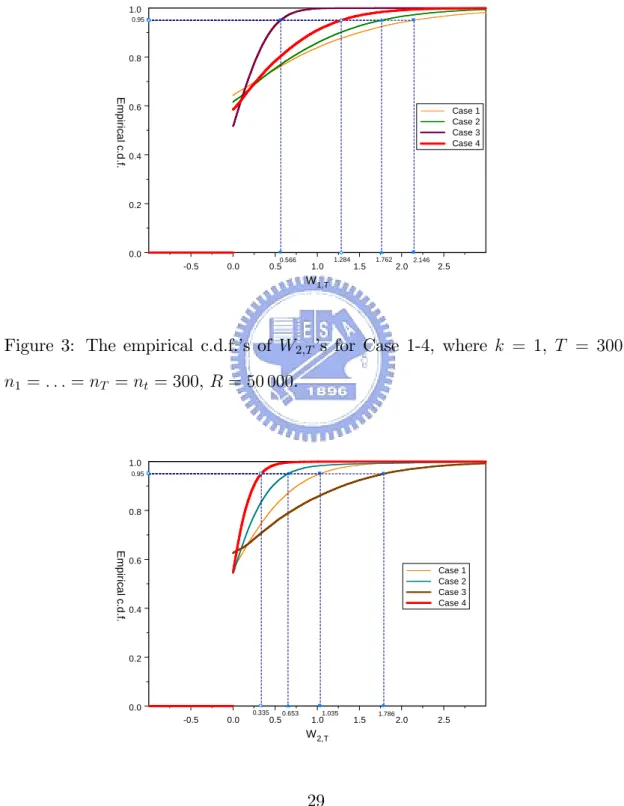
shown in Table 2, where u 2 f1; 2g, k = 1, T = 300, n1 = : : : = nT = 300, R = 50 000, and = 0:05. And the empirical c.d.f.’s of W1;T(y)’s and W2;T(y)’s for Cases 1-4 in Section 4 are shown in Figures 2 and 3, where k = 1, T = 300, n1 = : : : = nT = 300, R = 50 000.

Table 2: The values of Wu;T(y (u)

([R (1 )]))’s for Cases 1-4, where u 2 f1; 2g, k = 1,

T = 300, n1 = : : : = nT = nt = 300, R = 50 000, and = 0:05.

Case 1 Case 2 Case 3 Case 4

W1;T(y (1) ([R (1 )])) 2.146 1.762 0.566 1.284 W2;T(y (2) ([R (1 )])) 1.035 0.653 1.789 0.335

Figure 2: The empirical c.d.f.’s of W1;T’s for Case 1-4, where k = 1, T = 300, n1 = : : : = nT = nt= 300, R = 50 000. -0.5 0.0 0.5 1.0 1.5 2.0 2.5 W_1,T 0.0 0.2 0.4 0.6 0.8 1.0 E m p iri ca l c.d .f. Case 1 Case 2 Case 3 Case 4 2.146 1.762 0.566 1.284 0.95

Figure 3: The empirical c.d.f.’s of W2;T’s for Case 1-4, where k = 1, T = 300, n1 = : : : = nT = nt= 300, R = 50 000. -0.5 0.0 0.5 1.0 1.5 2.0 2.5 W_2,T 0.0 0.2 0.4 0.6 0.8 1.0 E m p iri ca l c.d .f. Case 1 Case 2 Case 3 Case 4 1.035 0.653 1.786 0.335 0.95

7

Let Pin denote the false-alarm rate, i.e., the probability that an out-of-control signal occurs when the manufacturing process is in control. Conventionally, Pin is taken to be 2 ( 3) ( 0:002 699 8), where is the c.d.f. of the standard normal distribution. In this section, utilizing the LR method, a Bayesian (or an empirical Bayes) monitoring scheme for the manufacturing process is proposed when F =

F 0 2 fF : 2 g for some known (or unknown) 0 2 . The main reason for

using the LR test is that it often has a higher power than other tests when the alternative hypothesis is true, which corresponds to a better detecting power in monitoring the process when the process is out of control.

In order to monitor the manufacturing process at time t (> T ), suppose that the response vector yt is observed. Then we are interested in testing whether or not the manufacturing process is in control at time t. Recall that F t is the prior

c.d.f. of t and that F( ) is the set of all c.d.f.’s on .

7.1

In this subsection, consider the case where F = F 0 2 fF : 2 g for some

known 0 _{2 . To monitor the manufacturing process at time t, the null hypothesis} H0: F t = F 0 versus the alternative H1: F t 6= F 0, i.e., F t 2 F( )nfF 0g, is

tested.

List all the elements of the sample space Ynt of yt by fy

(1)

t ; : : : ; y

(jYntj)

t g, where

jYntj (= (nt+ k)!=(nt!k!)) is the number of elements in Ynt. Regard F t as the

unknown parameter of interest in F( ). Then the unknown parameter of inter-est is non-parametric. Let `(F t; yt) ( log[f (yt; F t)]) denote the log-likelihood

function of F t given yt. Note that `(F _t; yt) = log Z f (ytj t) dF t( t) log Z sup t2 f (ytj t) dF t( t) = log Z f (ytj t)j _t=yt=nt dF t( t) = log h f (ytj t)j _t=yt=nt i ;

where the binomial/multinomial likelihood f (ytj t)for tgiven ytattains its max-imum at t = yt=nt: Thus, the MLE ^F t of F t given yt has p.m.f. 1fyt=ntg and

sup

F _t2F( )

`(F <sub>t</sub>; yt) = `(F t; yt)jF _t= ^F _t ` F^ t; yt = log f (ytj t)j t=yt=nt :

Let Wt; 0(y_t) denote the corresponding LR statistic, where

W_t; 0(y_t) = 2 log f (y_tj _t)j t=yt=nt ` 0_{; y} t (49) with P (f0 < Wt; 0(y_t) <1g; F_y t; 0) = 1.

The size PinLR test and a control chart of monitoring the LR statistic Wt; 0(y_t)

can be constructed as follows: Let (yt;(1); : : : ; yt;(jYntj))be a permutation of (y

(1) t ; : : :, y(jY_t ntj))such that Wt; 0(yt;(1)) : : : Wt; 0(yt;(jYntj)). Note that Wt; 0(yt)is a dis-crete random variable. If a deterministic upper control limit is used, a pre-speci…ed false-alarm rate Pin (2 (0; 1)), e.g., 2 ( 3), is nearly impossible to attain. How-ever, there is no problem to attain any pre-speci…ed false-alarm rate based on the concept of a randomized-upper-control-limit approach proposed in Shiau et al. (2005). To …nd the randomized upper control limit ( RU CL 0), we start

ac-cumulating the right tail probability from Wt; 0(y_t;(jY

such that P (fWt; 0(y_t) W_t; 0(y_t;(r))g; F_y

t; 0) Pin. Denote this r by m 0, i.e.,

m 0 = max r: P W_t; 0(y_t) W_t; 0 y_t;(r) ; F_y

t; 0 Pin : (50)

If P (fWt; 0(y_t) W_t; 0(y_t;(m

0))g; Fyt; 0) = Pin, which is nearly impossible, then

there is no need for randomization and Wt; 0(y_t;(m

0))is the upper control limit (

U CL 0). If P (fW_t; 0(y_t) W_t; 0(y_{t;(m 0)})g; F_y

t; 0) > Pin, then Wt; 0(yt;(m 0)) =

RU CL 0. Note that there may be more than one y_t;(r) such that W_t; 0(y_t;(r)) =

RU CL 0. Let m 0_;L, m 0_;U 2 f1; : : : ; jY_n tjg such that W_t; 0 y_t;(m 0;L 1) < Wt; 0 yt;(m 0;L) = RU CL 0 = Wt; 0 yt;(m 0;U) < W_t; 0 y_t;(m 0;U+1) ;

where Wt; 0(y_t;(0)) 0 and W_t; 0(y_t;(jY

ntj+1)) 1. Then the randomization is

done by signaling an out-of-control alarm with probability

P_in; 0_{;RU CL} = Pin P (fWt; 0(y_t) > RU CL 0g; F_y t; 0) P (_fWt; 0(y_t) = RU CL 0g; F_y t; 0) = Pin PjYntj r=m _0;U+1 P (fWt; 0(y_t) = W_t; 0(y_t;(r))g; F_y t; 0) Pm _0;U r=m _0;L P (fWt; 0(y_t) = W_t; 0(y_t;(r))g; F_y t; 0) :(51) This leads to Pin = P Wt; 0(yt) > RU CL 0 ; F_y t; 0 +P_in; 0_{;RU CL} P W_t; 0(y_t) = RU CL 0 ; F_y t; 0

randomiza-tion.

The monitoring scheme is as follows: If Wt; 0(y_t) > RU CL 0, then the null

hypothesis H0: F t = F 0 is rejected and the manufacturing process is declared

to be out of control at time t; if W_t; 0(y_t) < RU CL 0, then the null hypothesis

H0: F t = F 0 is not rejected and the manufacturing process is declared to be

in control at time t; if W_t; 0(y_t) = RU CL 0, then, with probability P_in; 0_{;RU CL},

the null hypothesis H0: F t = F 0 is rejected and the manufacturing process is

declared to be out of control at time t.

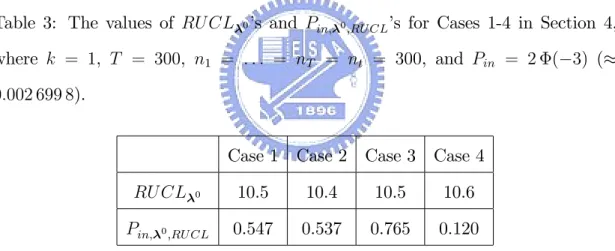
The corresponding values of RU CL 0’s and P_in; 0_{;RU CL}’s for Cases 1-4 in

Sec-tion 4 are shown in Table 3, where k = 1, T = 300, n1 = : : : = nT = nt = 300, and Pin = 2 ( 3) ( 0:002 699 8).

Table 3: The values of RU CL 0’s and P_in; 0_{;RU CL}’s for Cases 1-4 in Section 4,

where k = 1, T = 300, n1 = : : : = nT = nt = 300, and Pin = 2 ( 3) (

0:002 699 8).

Case 1 Case 2 Case 3 Case 4

RU CL 0 10.5 10.4 10.5 10.6

P_in; 0_{;RU CL} 0.547 0.537 0.765 0.120

7.2

In this subsection, consider the case where F = F 0 2 fF : 2 g for some

unknown 0 _{2 . To monitor the manufacturing process at time t (> T ), the null} hypothesis H0: F t = F 0 versus the alternative H1: F t 6= F 0 is tested.

The LR statistic Wt; 0(y_t) proposed in Section 7.1 for known 0 can be

esti-mated by Wt; 0(y_t)j 0_{= ^} ( W_t;^(y_t)), where ^ is the MLE of given y and

W_t;^(yt) = 2 n

log f (ytj t)j t=yt=nt ` ^; yt

o

(52)

with P (f0 < Wt;^(yt) < 1g; Fyt; 0) = 1. Note that ^ =

0

+ Op(1= p

T ) as T _{! 1, which implies that Wt;^}(yt) = Wt; 0(y_t) + O_p(1=

p

T )_{as T ! 1.}

An empirical Bayes monitoring scheme can be constructed by replacing the

unknown 0 by ^ in the Bayesian monitoring scheme described in Section 7.1,

where RU CL 0 and P_in; 0_{;RU CL} are estimated by RU CL 0j 0_{= ^} ( RU CL_^) and

P_in; 0_{;RU CL}j 0_{= ^} ( P_{in; ^ ;RU CL}), respectively.

To see how the additional estimation error resulting from the empirical Bayes approach a¤ects the performance of the monitoring scheme, the Kullback-Leibler divergence d(F 0; F_^) between F 0 and F_^ can be used as a measure of how close

F^ is to F 0, where F_^ F j = ^ and d (F 0; F_^) Z log ( t; )j = 0 ( t; )j _{= ^} ( t; )j = 0d t Z log " ( t; 0) ( t; ^) # ( t; 0) d t: (53)

When there is no closed-form formula for d(F 0; F_^), it can be numerically

evaluated as follows: First simulate an i.i.d. sample f (1)1 ; : : : ;

(R1)

1 g of size R1, e.g., R1 = 50 000, from the in-control prior c.d.f. F 0 and then numerically

evalu-ate d(F 0; F_^)by ^ d (F 0; F_^) 1 R1 R1 X r=1 log " ( t; 0) ( t; ^) # t= (r)1 : (54)

One way to numerically evaluate the quantile of d(F 0; F_^) for 2 (0; 1)

is as follows: First simulate an i.i.d. sample fy(1)_{; : : : ; y}(R)

g, e.g., R = 50 000, from the in-control marginal c.d.f. Fy; 0. Let (y₍₁₎; : : : ; y_(R)) be a permutation

of (y(1)_{; : : : ; y}(R)_{) such that ^d(F} 0; F_{^ (y} (1))) : : : ^ d(F 0; F_{^ (y} (R))). Then the

quantile of d(F 0; F_^) can be estimated by ^d(F 0; F_{^ (y}

([R ]))), where [R ] is the

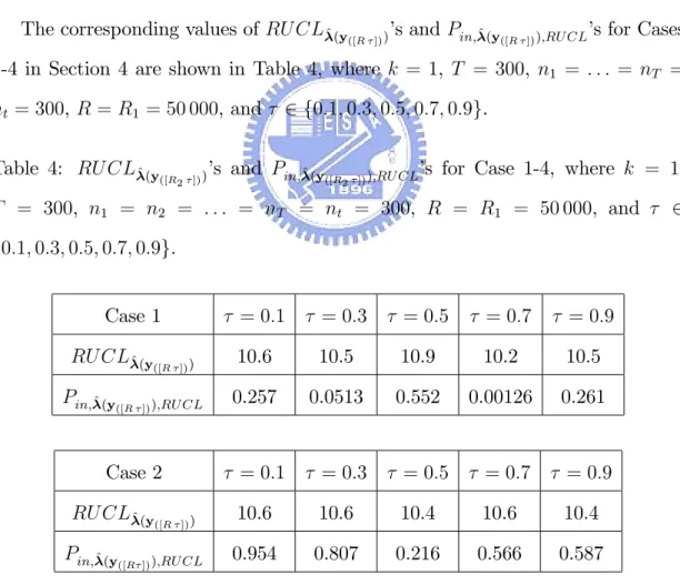
largest integer less than or equal to R . The corresponding values of RU CL_{^ (y}

([R ]))’s and Pin; ^ (y([R ]));RU CL’s for Cases

1-4 in Section 4 are shown in Table 4, where k = 1, T = 300, n1 = : : : = nT = nt = 300, R = R1 = 50 000, and 2 f0:1; 0:3; 0:5; 0:7; 0:9g.

Table 4: RU CL_{^ (y}

([R2 ]))’s and Pin; ^ (y([R2 ]));RU CL’s for Case 1-4, where k = 1,

T = 300, n1 = n2 = : : : = nT = nt = 300, R = R1 = 50 000, and 2 f0:1; 0:3; 0:5; 0:7; 0:9g. Case 1 = 0:1 = 0:3 = 0:5 = 0:7 = 0:9 RU CL_{^ (y} ([R ])) 10.6 10.5 10.9 10.2 10.5 P_{in; ^ (y} ([R ]));RU CL 0.257 0.0513 0.552 0.00126 0.261 Case 2 = 0:1 = 0:3 = 0:5 = 0:7 = 0:9 RU CL_{^ (y} ([R ])) 10.6 10.6 10.4 10.6 10.4 P_{in; ^(y} ([R ]));RU CL 0.954 0.807 0.216 0.566 0.587

Case 3 = 0:1 = 0:3 = 0:5 = 0:7 = 0:9 RU CL_^(y ([R ])) 10.5 10.3 10.3 10.5 10.6 P_{in; ^ (y} ([R ]));RU CL 0.688 0.0511 0.433 0.840 0.602 Case 4 = 0:1 = 0:3 = 0:5 = 0:7 = 0:9 RU CL_{^ (y} ([R ])) 10.5 10.4 10.7 10.5 10.3 P_{in; ^ (y} ([R ]));RU CL 0.346 0.506 0.353 0.449 0.553

From Tables 3 and 4, it is easily seen that all of RU CL_^(y

([R ]))’s are close

to RU CL 0, but P

in; ^(y([R ]));RU CL’s are not necessarily close to Pin; 0;RU CL for

Cases 1-4.

8

In this section, the performance of the proposed process monitoring scheme is studied in terms of the average run length. Let ARL0 denote the average run length for an out-of-control signal to occur when the manufacturing process is in control. Recall that Pin is the false-alarm rate, i.e., the probability that an out-of-control signal occurs when the manufacturing process is in out-of-control. Then ARL0 = 1=Pin. When Pin = 2 ( 3) ( 0:002 699 8), ARL0 = 1=[2 ( 3)] ( 370:40). Let ARL1 denote the average run length for an out-of-control signal to occur when the manufacturing process is out of control. Let Pout denote the correct-alarm rate, i.e., the probability that an out-of-control signal occurs when the manufacturing process is out of control. Similarly, ARL1 = 1=Pout.

8.1

In this subsection, consider the case where F = F 0 2 fF : 2 g for some

known 0 _{2 . To monitor the manufacturing process at time t, the monitoring}

scheme proposed in Section 7.1 is used for the null hypothesis H0: F t = F 0

versus the alternative H1: F t 6= F 0.

Set ARL0 ARL0; 0, P_in P_in; 0, ARL₁ ARL_1; 0_;F

t, and Pout Pout; 0_;F

t.

When Pin; 0 is pre-speci…ed to be 2 ( 3) ( 0:002 699 8),

ARL_0; 0 = 1 P_in; 0 = 1 2 ( 3) 370:40: (55) When F t 6= F 0, P_out; 0_;F t = P Wt; 0(y_t) > RU CL 0 ; F_y t +P_in; 0_{;RU CL} P W_t; 0(y_t) = RU CL 0 ; F_y t ; (56)

where all of W_t; 0(y_t), RU CL 0, and P_in; 0_{;RU CL} are de…ned in Section 7.1 and

Fyt is de…ned in Section 3.

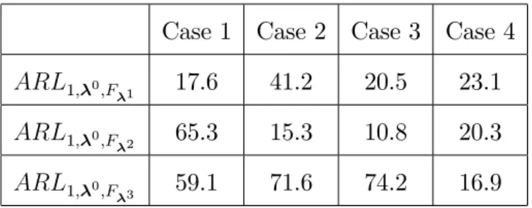
The corresponding values of Pout; 0_;F

i’s, and ARL1; 0;F i’s for Cases 1-4 in

Section 4 are shown in Tables 5 and 6, where k = 1, T = 300, n1 = : : : = nT = nt = 300, and i 2 f1; 2; 3g.

Case 1: 1 = (log(1=4); log(80); log(20); 2:210; log[1=(0:210)2_])T_, 2 _{= (log(1=} 9); log(90); log(10); 1:552; log[1=(0:220)2_])T_{, and} 3 _{= (log(4=21); log(80); log(20);}

0:503; log[1=(0:216)2_])T_.

Case 2: 1 = (log(9=11); log(85); log(15); 0:510; log[1=(0:210)2_])T_, 2 = (log(11=9); log(72); log(18); 2:030; log[1=(0:210)2_])T_{, and} 3

log(20); 0:203; log[1=(0:202)2_])T_.

Case 3: 1 = (log(2=3); log(65); log(35); 0:110; log[1=(0:210)2])T, 2 = (log(1); log(70); log(30); 2:005; log[1=(0:253)2])T, and 3 = (log(3=2); log(60); log(40); 0:2 03; log[1=(0:202)2_])T_.

Case 4: 1 = (log(4); log(70); log(20); 1:510; log[1=(0:210)2_])T_, 2 _{= (log(3);} log(88); log(22); 1:203; log[1=(0:220)2_])T_{, and} 3 _{= (log(83=17); log(80); log(20);} 1:203; log[1=(0:041)2_])T_.

Table 5: The values of Pout; 0_;F

i’s for Cases 1-4, where k = 1, T = 300, n1 = : : : =

nT = nt = 300, and i 2 f1; 2; 3g.

Case 1 Case 2 Case 3 Case 4

P_out; 0_;F 1 0.0568 0.024 0.0487 0.0434 P_out; 0_;F 2 0.0153 0.0652 0.0929 0.0492 P_out; 0_;F 3 0.0169 0.0140 0.0135 0.0590

Table 6: The values of ARL_1; 0_;F

i’s for Cases 1-4, where k = 1, T = 300, n1 =

: : : = nT = nt= 300, and i 2 f1; 2; 3g.

Case 1 Case 2 Case 3 Case 4

ARL_1; 0_;F 1 17.6 41.2 20.5 23.1 ARL_1; 0_;F 2 65.3 15.3 10.8 20.3 ARL_1; 0_;F 3 59.1 71.6 74.2 16.9

8.2

In this subsection, consider the case where F = F 0 2 fF : 2 g for some

unknown 0 _{2 . To monitor the manufacturing process at time t, the monitoring} scheme proposed in Section 7.2 is used for the null hypothesis H0: F t = F 0

versus the alternative H1: F t 6= F 0.

Set ARL0 ARL0; 0_;^, P_in P_in; 0_;^, ARL₁ ARL_1; 0_{;^ ;F}

t, and Pout

P_out; 0_{;^ ;F}

t. When ^ =

0

, which is nearly impossible, we have P_in; 0_;^ = P_in; 0

and P_out; 0_{;^ ;F} t

= P_out; 0_;F

t, where both Pin;

0 and P_out; 0_;F

t are de…ned in

Sec-tion 8.1. When ^ 6= 0, we have

P_in; 0_;^ = P n W_t;^(yt) > RU CL^ o ; F_yt; 0 +P_{in;^;RU CL} P nW_t;^(yt) = RU CL^ o ; F_yt; 0 (57) and P_out; 0_{;^ ;F} t = P n W_t;^(yt) > RU CL^ o ; Fyt +P_{in; ^ ;RU CL} P nW_t;^(yt) = RU CL^ o ; Fyt ; (58)

where all of W_t;^(yt), RU CL^, and P_{in; ^;RU CL} are de…ned in Section 7.2 and both F_yt; 0 and F_y

t are de…ned in Section 3.

To see how the additional estimation error resulting from the empirical Bayes approach a¤ects the performance of the average run length, the Kullback-Leibler divergence d(F 0; F_^)between F 0 and F_^ de…ned in Section 7.2 can be used as a

measure of how close F^ is to F 0. See Section 7.2 for details.

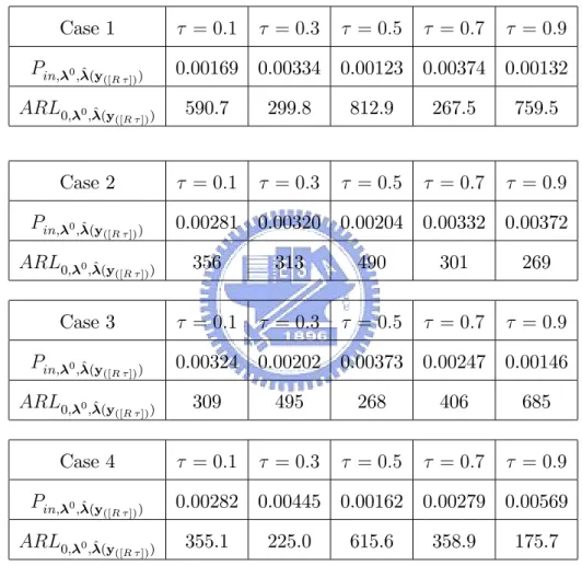
1-4 in Section 4 are shown in Table 7, where k = 1, T = 300, n1 = : : : = nT = nt = 300, R = R1 = 50 000, and 2 f0:1; 0:3; 0:5; 0:7; 0:9g.

Table 7: The values of P_in; 0_{;^ (y}

([R2 ]))’s and ARL0; 0;^(y([R ]))’s for Cases 1-4, where

k = 1, T = 300, n1 = : : : = nT = nt = 300, R = R1 = 50 000, and 2 f0:1; 0:3; 0:5; 0:7; 0:9g. Case 1 = 0:1 = 0:3 = 0:5 = 0:7 = 0:9 P_in; 0_{;^ (y} ([R ])) 0.00169 0.00334 0.00123 0.00374 0.00132 ARL_0; 0_{;^ (y} ([R ])) 590.7 299.8 812.9 267.5 759.5 Case 2 = 0:1 = 0:3 = 0:5 = 0:7 = 0:9 P_in; 0_{;^ (y} ([R ])) 0.00281 0.00320 0.00204 0.00332 0.00372 ARL_0; 0_{;^ (y} ([R ])) 356 313 490 301 269 Case 3 = 0:1 = 0:3 = 0:5 = 0:7 = 0:9 P_in; 0_{;^ (y} ([R ])) 0.00324 0.00202 0.00373 0.00247 0.00146 ARL_0; 0_{;^ (y} ([R ])) 309 495 268 406 685 Case 4 = 0:1 = 0:3 = 0:5 = 0:7 = 0:9 P_in; 0_{;^ (y} ([R ])) 0.00282 0.00445 0.00162 0.00279 0.00569 ARL_0; 0_{;^ (y} ([R ])) 355.1 225.0 615.6 358.9 175.7

The corresponding values of P_out; 0_;^(y

([R ]));F i’s and ARL1; 0;^ (y([R ]));F i’s for

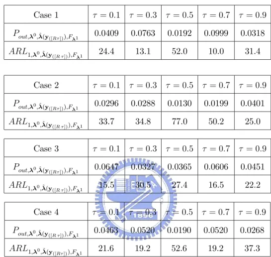
Cases 1-4 in Section 4 are shown in Tables 8-10, where k = 1, T = 300, n1 = : : : = nT = nt = 300, R = R1 = 50 000, 2 f0:1; 0:3; 0:5; 0:7; 0:9g, and i 2 f1; 2; 3g. Table 8: The values of P_out; 0_{;^ (y );F} ’s and ARL_1; 0_{;^ (y );F} ’s for Cases

1-4, where k = 1, T = 300, n1 = : : : = nT = nt = 300, R = R1 = 50 000, and 2 f0:1; 0:3; 0:5; 0:7; 0:9g. Case 1 = 0:1 = 0:3 = 0:5 = 0:7 = 0:9 P_out; 0_{;^ (y} ([R ]));F 1 0.0409 0.0763 0.0192 0.0999 0.0318 ARL_1; 0_;^(y ([R ]));F 1 24.4 13.1 52.0 10.0 31.4 Case 2 = 0:1 = 0:3 = 0:5 = 0:7 = 0:9 P_out; 0_{;^ (y} ([R ]));F 1 0.0296 0.0288 0.0130 0.0199 0.0401 ARL_1; 0_;^(y ([R ]));F 1 33.7 34.8 77.0 50.2 25.0 Case 3 = 0:1 = 0:3 = 0:5 = 0:7 = 0:9 P_out; 0_{;^ (y} ([R ]));F 1 0.0647 0.0327 0.0365 0.0606 0.0451 ARL_1; 0_;^(y ([R ]));F 1 15.5 30.5 27.4 16.5 22.2 Case 4 = 0:1 = 0:3 = 0:5 = 0:7 = 0:9 P_out; 0_{;^ (y} ([R ]));F 1 0.0463 0.0520 0.0190 0.0520 0.0268 ARL_1; 0_{;^ (y} ([R ]));F 1 21.6 19.2 52.6 19.2 37.3

Table 9: The values of P_out; 0_{;^ (y}

([R ]));F 2’s and ARL1; 0;^ (y([R ]));F 2’s for Cases

1-4, where k = 1, T = 300, n1 = : : : = nT = nt = 300, R = R1 = 50 000, and 2 f0:1; 0:3; 0:5; 0:7; 0:9g. Case 1 = 0:1 = 0:3 = 0:5 = 0:7 = 0:9 P_out; 0_;^(y ([R ]));F 2 0.0126 0.0184 0.00802 0.0218 0.0108 ARL_1; 0_;^(y ([R ]));F 2 79.5 54.4 125 46.0 92.8

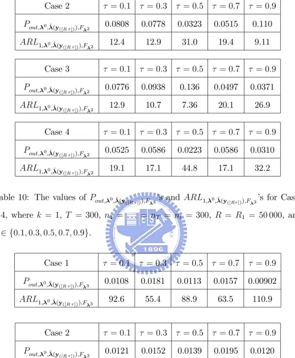
Case 2 = 0:1 = 0:3 = 0:5 = 0:7 = 0:9 P_out; 0_{;^ (y} ([R ]));F 2 0.0808 0.0778 0.0323 0.0515 0.110 ARL_1; 0_;^(y ([R ]));F 2 12.4 12.9 31.0 19.4 9.11 Case 3 = 0:1 = 0:3 = 0:5 = 0:7 = 0:9 P_out; 0_{;^ (y} ([R ]));F 2 0.0776 0.0938 0.136 0.0497 0.0371 ARL_1; 0_;^(y ([R ]));F 2 12.9 10.7 7.36 20.1 26.9 Case 4 = 0:1 = 0:3 = 0:5 = 0:7 = 0:9 P_out; 0_{;^ (y} ([R ]));F 2 0.0525 0.0586 0.0223 0.0586 0.0310 ARL_1; 0_;^(y ([R ]));F 2 19.1 17.1 44.8 17.1 32.2

Table 10: The values of P_out; 0_{;^ (y}

([R ]));F 3’s and ARL1; 0;^ (y([R ]));F 3’s for Cases

1-4, where k = 1, T = 300, n1 = : : : = nT = nt = 300, R = R1 = 50 000, and 2 f0:1; 0:3; 0:5; 0:7; 0:9g. Case 1 = 0:1 = 0:3 = 0:5 = 0:7 = 0:9 P_out; 0_{;^ (y} ([R ]));F 3 0.0108 0.0181 0.0113 0.0157 0.00902 ARL_1; 0_;^(y ([R ]));F 3 92.6 55.4 88.9 63.5 110.9 Case 2 = 0:1 = 0:3 = 0:5 = 0:7 = 0:9 P_out; 0_{;^ (y} ([R ]));F 3 0.0121 0.0152 0.0139 0.0195 0.0120 ARL_1; 0_;^(y ([R ]));F 3 82.8 65.9 72.1 51.3 83.2

Case 3 = 0:1 = 0:3 = 0:5 = 0:7 = 0:9 P_out; 0_{;^ (y} ([R ]));F 3 0.0199 0.00786 0.00911 0.0182 0.0121 ARL_1; 0_{;^ (y} ([R ]));F 3 50.3 127 109 55.1 82.6 Case 4 = 0:1 = 0:3 = 0:5 = 0:7 = 0:9 P_out; 0_{;^ (y} ([R ]));F 3 0.0627 0.0695 0.0282 0.0695 0.0383 ARL_1; 0_{;^ (y} ([R ]));F 3 16.0 14.4 35.5 14.4 26.1

From Tables 8-10, there is no pattern that the values of P_in; 0_;^ and P_out; 0_{;^ ;F} i

for Case 1-Case 4 increase as the Kullback-Leibler divergence d(F 0; F_^)increases,

where k = 1, T = 300, n1 = : : : = nT = nt = 300, R = R1 = 50 000, and

i_{2 f1; 2; 3g.}

9

In the paper, …rst, a two-components mixture prior parametric family for the in-control prior distribution is proposed in a manufacturing process. Then an em-pirical Bayes approach is proposed when there are available in-control categorical data generated from the manufacturing process. As an illustration, an example of the proposed empirical Bayes model is introduced. For the purpose of model building, the goodness of …t and the simpli…cation of the proposed model are dis-cussed. Utilizing the likelihood ratio method, both Bayesian and empirical Bayes monitoring techniques are proposed as the main purpose of the paper. Finally, the performance of the proposed process monitoring scheme is studied in terms of the average run length to show the robustness of the methodology.

APPENDIX

All of nodes and weights of the Hermite polynomial of 32 degrees are shown in the following table. This table is obtained from the following website:

http://www.efunda.com/math/num_integration/…ndgausshermite.cfm

No. i abscissas xi weights wi

1 7:12581390983 7:31067642754 10 23 2 6:40949814928 9:23173653482 10 19 3 5:81222594946 1:19734401957 10 15 4 5:27555098664 4:21501019491 10 13 5 4:77716450334 5:93329148347 10 11 6 4:30554795347 4:09883215841 10 9 7 3:85375548542 1:57416779440 10 7 8 3:41716749282 3:65058512533 10 6 9 2:99249082501 5:41658405999 10 5 10 2:57724953773 5:36268365495 10 4 11 2:16949918361 3:65489032677 10 3 12 1:76765410946 1:75534288315 10 2 13 1:37037641095 6:04581309559 10 2 14 0:97650046359 1:51269734077 10 1 15 0:58497876544 2:77458142303 10 1 16 0:19484074157 3:75238352593 10 1

No. i abscissas xi weights wi 17 0:19484074157 3:75238352593 10 1 18 0:58497876544 2:77458142303 10 1 19 0:97650046359 1:51269734077 10 1 20 1:37037641095 6:04581309559 10 2 21 1:76765410946 1:75534288315 10 2 22 2.16949918361 3:65489032677 10 3 23 2:57724953773 5:36268365495 10 4 24 2:99249082501 5:41658405999 10 5 25 3:41716749282 3:65058512533 10 6 26 3:85375548542 1:57416779440 10 7 27 4:30554795347 4:09883215841 10 9 28 4:77716450334 5:93329148347 10 11 29 5:27555098664 4:21501019491 10 13 30 5:81222594946 1:19734401957 10 15 31 6:40949814928 9:23173653482 10 19 32 7:12581390983 7:31067642754 10 23

REFERENCES

1. Agresti, A. (2002). Categorical Data Analysis, 2nd ed. John Wiley & Sons, New York.

3. Chen, C.-R. and Liu, C.-Y. (2005). A Model Selection Technique Between Two Empirical Bayes Models for Categorical Data. Technical Report, Insti-tute of Statistics, National Chiao Tung University, Hsinchu, Taiwan.

4. Chen, C.-R., Shiau, J.-J. H., Liao, H.-H., and Feltz, C. J. (2004). A process monitoring technique for categorical data under the beta-binomial/Dirichlet-multinomial empirical Bayes model. Technical Report, Institute of Statistics, National Chiao Tung University, Hsinchu, Taiwan.

5. Chen, C.-R., Shiau, J.-J. H., Lin, T.-Y., and Feltz, C. J. (2005). A process monitoring technique for categorical data under the transformed-normal-binomial/multinomial empirical Bayes model. Technical Report, Institute of Statistics, National Chiao Tung University, Hsinchu, Taiwan.

6. Fahrmeir, A. and Tutz, G. (2001). Multivariate Statistical Modelling Based on Generalized Linear Models, 2nd ed. Springer-Verlag, New York.

7. Gelman, A., Carlin, J. B., Stern, H. S., and Rubin, D. B. (2004). Bayesian Data Analysis, 2nd ed. Chapman & Hall/CRC, Boca Raton.

8. Johnson, N. L., Kotz, S., and Balakrishnan, N. (1997). Discrete Multivariate Distributions. John Wiley & Sons, New York.

9. McCullagh, P. and Nelder, J. A. (1989). Generalized Linear Models, 2nd ed. Chapman and Hall, London.

10. McLachlan, G. J. and Peel, D. (2000). Finite Mixture Models. John Wiley & Sons, New York.

11. O’Hagan, A. and Forster, J. (2004). Kendall’s Advanced Theory of Statistics, Volume 2B: Bayesian Inference, 2nd ed. Arnold, London.

12. Shiau, J.-J. H., Chen, C.-R., and Feltz, C. J. (2005). An empirical Bayes process monitoring technique for polytomous data. Quality and Reliability Engineering International, 21, 13-28.

13. Yousry, M. A., Sturm, G. W., Feltz, C. J., and Noorossana, R. (1991). Process monitoring in real time: empirical Bayes approach - discrete case. Quality and Reliability Engineering International, 7, 123-132.