Determinants of Return on Equity of enterprises in the real estate industry listed on Ho Chi Minh Stock Exchange

(1)

College of Management

I-Shou University

Master Thesis

Determinants of Return on Equity

of enterprises in the real estate industry listed on

Ho Chi Minh Stock Exchange

Advisor: Ph.D. Yeh, Chao – Hui

Graduate Student: Nguyen, Thi Lan Phuong

(2)

(3)

Acknowledgment

Two years have been passed so fast. I have obtained so many experiences in academic study and my personal life. Obviously, I would not be here without support from many people.

I would like to say thank you for my family, mom, dad and my sister. Thank you for your support and make me laugh when I felt tired with these. Third, I would like to express my gratitude and appreciation for my supervisor, PhD. Yeh Chao Hui for his help and guidance through all the process. I would like to say thank you for all the committee Prof. Lan Yu Chen and Prof. Lin Chu-hsiung for their valuable opinions and contribution comments.

In addition, I am thankful for my entire classmate, my friends who help me for these two years. I will never forget all the memories we’ve been through together. Thanks to all those people who participate in my collecting data of my research and those who give me comments and suggestions to carry out the study.

Kaohsiung, June 2017

(4)

Abstract

The real estate market is a market that promotes the economic, social development of Vietnam and contributes to improving the living standard of the population. The objective of this research is to diagnose the financial variables that are determinants of Return on Equity in real estate firms. The direction of the dissertation was supplied by taking data from 2007 to 2016 of 35 enterprises of Ho Chi Minh Stock Exchange.

This study used Eview software. Random Effect Model with panel data is used to test relationship between variables. The results showed that except Current Ratio, the remaining financial ratios show statistical significance for the firms ROE. The findings concerning the financial firms indicate that only Risk is statistically negative significant, while the remaining financial ratios show statistic positive significance with ROE.

(5)

List of Abbreviations

1 ASSETS Total Assets

2 AT Asset Turnover

3 CR Current Ratio

4 FEM Fixed Effects Models

5 GLS Generalized Least Squares

6 HOSE Ho Chi Minh Stock Exchange

7 LEV Leverage

8 MPT Modern Portfolio Theory

9 NPM Net Profit Margin

10 OLS Ordinary Least Squares

11 REM Random Effects Models

12 RISK Risk Ratio

13 ROA Return on Asset

14 ROE Return on Equity

15 TIE Times Interest Earned

(8)

List of Tables

Table 3.1 Description of variables in model testing………. 17

Table 4.1 Output of Descriptive Statistics……….…………... 21

Table 4.2 Correlation matrix……….……… 23

Table 4.3 Autocorrelation regression analysis………... …….. 24

Table 4.4 Autocorrelation analysis result……….……… 24

Table 4.5 Heteroskedasticity regression analysis………. 25

Table 4.6 Heteroskedasticity analysis result………. 25

Table 4.7 Output of Hausman Test……….……….. 26

Table 4.8 Output of Random Effect Model……….………….. 27

(9)

List of Figures

Figure 1.1 Research flowchart…...4 Figure 2.1 Du-Pont Formula …... 7

(10)

Chapter 1 INTRODUCTION

The objective of first chapter is to introduce the research background of the study, the situation of economics of Vietnam as well as the condition of Vietnamese real estate enterprises. In addition, this chapter also explains problem identification, the essential of researching Return on Equity to attract capital and discusses the scope of research, research objective. Form that, author give research questions to satisfy research purposes. The author hope this dissertation will have some contributions for further researches.

1.1 Research background

According to data reported to World Bank (2016), since joined World Trade Organization, GDP of Vietnam has a significantly increase from 66.37 USD Billion in 2005 to 193.60 USD Billion in 2015. Being a member of WTO, there are many opportunities as well as challenges to economic integration process of Vietnam (Quan & Ly, 2015). In that context, the real estate market became one of the most important markets which attract more attention and investment of individuals and society, in specific real estate market accounts 34.2% in market capitalization of Vietnam (HOSE, 2015). Real estate market is also the market inputs of the production process beside the capital market and the labor market. However, property market is not simple, it is complex with erratic progress. Due to this market accounts for a large capital, market fluctuation negatively will have a strong influence on economy.

In recent years, the real estate market in Vietnam have developed instability, even have time “freeze” affecting the macro-economic balance which leading negative impact on the background economy. Many real estate businesses and trading real estate services were difficult, especially for small and medium sized companies. From end of 2013 to 2015, the real estate market has been in the recovery trend; for instance, liquidity improved and the number of successful transactions is increasing (Chu et al, 2015). Those are positive signs for the real estate market. However, according to Nguyen Tran Nam - Deputy Minister of Construction of Vietnam, although the market have positive signs in the transaction, the problem has not been solved completely. Therefore, firms in the sector require the effective business strategy to get high profit to the business. Vietnamese businesses actually are still in a vicious circle, no way out while the majority of projects under construction are in progress, too much property in stock causes difficult in capital rotation; therefore, investors do not have the capital to continue to build, customers also stop contributing capital. The access to funding difficultly forces these

(11)

firms have to borrow short-term loans at high interest rates. Moreover, businesses are unable to access medium and long-term funding as well as from other credit funds.

To solve this problem and to improve the efficiency of operation and reasonable capital management, businesses also need to consider the financial indicators. Financial indicators are tool for analysts find the trends of the business as well as investors, creditors and lenders check the financial health situation of enterprise. One of financial indicators plays an important role – an effective leverage in attracting capital is Return on Equity - ROE (Nguyen, 2009). ROE is a financial ratio that is used for comparisons between companies in order to assess profitability and to enable shareholders identify investment opportunities and establish the best suited to their return requirements (Popov & Roosenboom, 2009). This ratio is influenced by some factors such as Asset Turnover, Current liquidity ratios, Net Profit Margin ratio, total Assets and solvency. That is reason why author choose to study about ROE and factors affecting ROE of real estate companies to hope that providing appropriate solutions to improve ROE of this enterprises.

To know exactly about ROE of property entrepreneurs, we need to find the place where the data is clearly and be updated every moment. Ho Chi Minh Stock Exchange (HOSE) is the largest stock exchange in Vietnam and the secondary capital market. On July 10th 1998, the Prime Minister signed Decree No. 48/1998/ND-CP on stock and securities market and a Decision to set Ho Chi Minh City Securities Trading Center. After 9 years of growing and integrating into the global securities market, the government signed Decision No. 599/QD-TT on May 11th 2007 to transfer the Ho Chi Minh City Securities Trading Center to Ho Chi Minh Stock Exchange (HOSE). To be listed on the HOSE market, companies must satisfy all the conditions in capital and financial activities of publicity, ROE in most recent year was at least 5% and the company have to report a profit. Companies must regularly update the financial situation monthly, quarterly and annually. Therefore, HOSE is also a clearly and transparent financial channel for shareholders, investors consider buying shares and investing in industries in Vietnam.

Therefore, through this research, researcher aims to improve ROE and the factors that influence ROE through an analytical model to devise appropriate measures. That is why the author studied the topic: "Determinants of Return on Equity of enterprises in the real estate industry listed on HOSE".

(12)

1.2 Research questions

The target of this essay is want to find out determinants of Return on Equity (ROE) with regard to real estate companies listed on HOSE between 2007 and 2016. This research will study about the real estate market of Vietnam, the ROE and the factors affecting to ROE of this kind of companies and the relationship between research factors to companies. Besides that analyzing the current situation of ROE and its factors of companies help find the best solutions to improve the business performance of Vietnamese estate companies nowadays. Thus, research question for this study are:

1. What are factors affecting to ROE of the companies in the industry of real estate listed on HOSE?

2. How do these factors influence to ROE of the companies in the industry of real estate listed on HOSE?

1.3 Research significance

The research has examined the determinants of ROE of Vietnamese estate companies. The necessary of this research can be considered from two elements: theoretical contributions and practical implications. In theory, the study fixes an important gap in previous literature that is, exploring the determinants affecting to ROE in specific kinds of companies (real estate firms). Therefore, the findings of this research can supplement to the existing problems of the literature and can serve as a starting point on which future studies can be improved. On the practical side, in the context of fierce competition among real estate enterprises to attract investors and customers, this study can help firm managers to identify the important factors that may determine ROE of companies in order to build more strategy to attract capital and find methods how to improve their firms’ operations. Such information should help managers make decisions adjust the shortcomings for reaching and attracting investors. In the other hand, it also helps investors look right to choose and evaluate appropriate companies to invest; credit analysts to assess the ability of companies and securities analysts to the company's effectiveness, risk, and prospects.

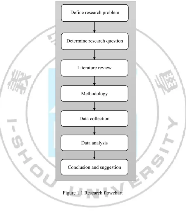
1.4 Research structure

Here is research structure described steps that author will conduct in next chapter in dissertation. Firstly, defining the problem and giving topic of research. Secondly, researching the literature review of each factor depends on previous research and finding out the gap of that studies as well as developing new model in this paper. Next is showing methodology from data

(13)

collection and analyzing the collected data. Last, giving conclusion after testing model of this problem and answering the research question as well as recommendation to improve the research quality.

Figure 1.1 Research flowchart Define research problem

Literature review Determine research question

Methodology

Data collection

Data analysis

(14)

Chapter 2 LITERATURE REVIEW

This chapter demonstrates the importance of using the financial ratio, classification of financial ratio; the definition of Return on Equity, the concept and theories as well as the necessary to analyze Return on Equity. Furthermore, the chapter is reviewed of some previous works of other researchers that related to the topic. In addition, it is given seven factors that affect to ROE, definition of each factor and some previous studies research of the relationship between ROE and some factors. All of them will be a fundamental to build the hypothesis of each factor.

2.1 Return on Equity (ROE)

This section explains the essential and types of financial ratio based on viewed of researchers and scholars. Next, giving definition of Return on Equity, explaining how assess it and the important of ROE in company with managers, investors and shareholders.

2.1.1 Financial ratio

Financial ratios include five different categories: liquidity, profitability, debt management, asset management and market value ratio (Gibson, 1982) that help to evaluate financial statement. Each type has different functionality to predict and study the financial situation of any company (Altman, 1968).

Liquidity ratio: The indicators in this category are calculated and used to determine

capability of particular business for paying the short-term obligation. Current ratio, quick ratio, cash ratio are represented to this kind of ratio.

Profitability ratio: The indicators said the overall profitability of the company, also shows

how effectiveness the property was used. Business financial theory has authorized two relative dimensions of profitability which are Return on Assets and Return on Assets. Both are used to diagnose a company's profitability (Stancu, 2007). Profit margin, ROE, ROA are showed profitability ratio.

Debt management ratio: it is said how does the company consider its assets to pay off its

debt as well as the capability of the company to pay off its long-term or short-term debt; it is also defined as an ability of the company to settle its all liabilities by available cash includes business risk and financial risk;. Financial risk is the risk related to the financial structure of the company (Nguyen, 2015). This ratio include total debt ratio, times interest earned, cash coverage.

(15)

Asset management ratio: extremely meaningful indicators for shareholders and investors

to consider whether the company is worth anywhere and allows creditors to predict ability to repay current liabilities and evaluation additional debt or the efficiency of using assets of the enterprises (Brigham, 2010) such as inventory turnover, receivables turnover, total asset turnover.

Market value ratio: which describe the stock price and show what the investor thinks about

the company and its prospects in the future like Price - earnings ratio, market - to - book ratio. In corporate financial reports, the analysis of ratio of profitability is very essential point. Managers and investors who analyze this ratios can assess the performance of the business, helping to make their invested decisions. Financial ratio is an important and effective tool however when using this ratio, it need to put in historical value of same firms or industries because the ratio is counted from accounting so different principle can make different results and based on business practices and cultures of enterprises’ country (Gibson, 2011). Wild (2009) also said that financial investigation is used to figure out the financial situation and performance of the company, in addition to the indicators used to evaluate the financial performance that its profitability in future. Financial indicators were used by interior and extraneous financial data users for having their economic selection. including investing, and performance evaluation decisions.

Some Western researches such as the studies of Altman (1968); Beaver, McNichols & Rhie (2005); Hossari (2006), Vietnamese studies also use both financial statement ratios and nonfinancial elements to search best ratios and find the reason of business failure. Harahap (2004) stated that financial ratios are collected from the financial reports or posts and comparison all to make this numbers be more meaningful and relevant. Financial indicators give this information related to the measurement of business quality and evaluate to decide whether to invest in support of a company (Zager, 2006). One explanation was given by Nissim & Penman (2001), the financial ratio is standard level to identify and measure differences in negative or positive financial operations and activities of employees in company. Nweze (2011) defined the analysis of financial statements using ratio analysis as putting two financial indicators together. It's more efficient to choose the right variables predetermined ratio which describes the advantages and disadvantages of the firm's financial situation (Tugas & Cisa, 2012). Managers have a duty to identify and control the decisive factors for the implementation of development, sustainable growth for a company (Kochhar, 1996; Cassar, 2004).

In financial accounting and reporting, it is generally demonstrated that there are assured relationships between the items shown in the accounts of profits and losses, in the annual report

(16)

as well as between components in the report. Therefore, the financial ratio is used as a means of expressing relationships in business situation. Ezeamama (2010) battles that indicators are effective tool to interpret the financial statement when correlated to a definitive or norm. Pandey (2010) shows the financial analysis is the process through analyzing the numbers to explore the strengths and weaknesses of the financial company, thereby instituting the relationship between the firms by the establishment correct relationships between items in the balance sheet and the profit and loss account of the company.

2.1.2 Definition of Return on Equity

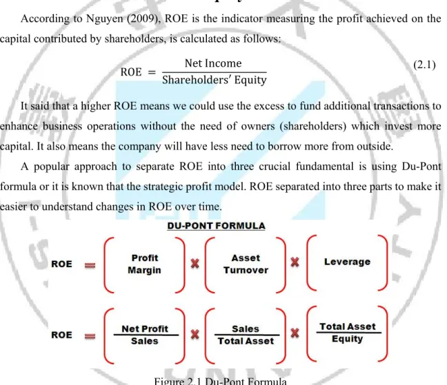
According to Nguyen (2009), ROE is the indicator measuring the profit achieved on the capital contributed by shareholders, is calculated as follows:

ROE Net Income Shareholders′ Equity

(2.1)

It said that a higher ROE means we could use the excess to fund additional transactions to enhance business operations without the need of owners (shareholders) which invest more capital. It also means the company will have less need to borrow more from outside.

A popular approach to separate ROE into three crucial fundamental is using Du-Pont formula or it is known that the strategic profit model. ROE separated into three parts to make it easier to understand changes in ROE over time.

Figure 2.1 Du-Pont Formula

The Du-Pont maintains the function of a firm’s profitability, asset utilization efficiency and financial leverage to analyze a ROE digit. In addition, Du-Pont model shows interactions between specific financial indicators is the ratio of operating profit and sales to determine profitability on invested capital. The equation also shows the relationship and impact of these factors are indicators of capital efficiency, which can set the appropriate decisions and

(17)

efficiently based on different level of impact of each different factors to increase profitability. If ROE is unsatisfactory by some measure, the Du-Pont identity tells the reason.

ROE is often used to analyze for comparison with the stock in the same industry, and the ratio supported to the decision what shares of company should buy. Return on Equity computes the return to common shareholders (Fraser & Ormiston, 2004). ROE is the best measure ability of company to maximize the profit from each investment contract. The higher ROE firm achieved, the stronger competitiveness of the company are.

2.1.3 Particular importance of Return on Equity

Greater importance is given to ROE because it is commonly used by investors when evaluating stock purchases and assessing the corporate performance (Acheampong, 2000). When the company only reaches ROE equivalent to bank interest, at a relative level, investors should revisit the profitability of the company, as if the company is only profitable at this level. No company will get a loan from the bank, since the interest on loans is enough to pay interest on a bank loan. Of course, here he just put the case the company has not yet borrowed the bank. According to Damodaran (2007), ROE “focuses on just the equity component of the investment. It relates the earnings left over for equity investors after debt services costs have been factored in to the equity invested in the asset”. However, the ROE does not describe the details of how much money will be returned to shareholders, but only indicates the profitability that company create based on shareholders’ equity (Berman et al., 2013). Even so, ROE still become the essential financial indicators that shareholders use so as to assess whether their investments are profitable or not (Dietrich & Wanzenried, 2009).

ROE is often a difference for companies with different age. The newly established companies usually have high ROE by deciding to allocate capital simpler. Long-standing companies, especially companies operating in industries with high capital concentration as communications, technology so the ROE are lower, because they are costly to create a contract revenue or profit. On the other hand, the ROE of the industry also is very different, so ROE should compare between similar businesses (in terms of size, product structure ...) or compared with the sector average. Likewise ROE is used as a measure of manager’s performance and define a manager´s remuneration, this can encourage them to invest more projects, which have higher than expected ROE, though those projects can be very risky for companies (Gadoiu, 2014).

(18)

2.1.4 Limitation of ROE

Assessing and measuring corporate financial performance is one of the most controversial and discussed issues in financial management. The use of tools to assess the financial performance of enterprises is important.

There are a lot of measures to measure corporate financial performance, but the most commonly used indicators in the studies can be divided into two main groups: first, using multiple accounting tools. Used in previous research, is the ratio between the results achieved (net income, net profit) and inputs (assets, capital, investment capital, equity Property). The second set of indicators, including market-based models. For the first set of indicators: To measure corporate financial performance, ROA and ROE are currently the two most widely used factors.

However, the value of these two factors may depend on how the "profit" indicator is derived. Profit before tax and interest (EBIT) are chosen by many researchers to account for these two factors (Hu & Izumida, 2008, Le & Buck, 2011, Wang & Xiao, 2011). Net profit plus interest (before or after tax) (Shah, Butt & Saeed, 2011; Thomsen & Pedersen, 2000), or simply net profit (LI, Sun & Zou, 2009). Meanwhile, the study said that the use of profit before tax, interest, wear and depreciation (EBITDA).

In summary, the group of factors based on book value is a view of the past or the short-term profitability of a firm (Hu & Izumida, 2008). Because factors such as ROA and ROE are effective indicators for current business results and reflect the value of profits earned in the past accounting periods. In addition, the norms of the first group do not provide a long-term perspective for shareholders and business leaders as they are historical and short-term measures (Jenkins, Ambrosini & Collier, 2011). Therefore, if having decision to purchase stock, it should be further examined other factors besides ROE like ROA, EPS,… In this study, the author conducted research on the impacts of determinants affecting to ROE of business cooperation.

2.2 Factors affecting to ROE

In this study, there are seven factors that affect to ROE such as Current Ratio, Asset Turnover, Leverage, Net Profit Margin, Time Interest Earned, Assets and Risk. This section shows the definition of each factor, the mathematic formula as well as the meaning of its. In addition, the prior of researchers’ hypothesis are given as foundation to me to build my hypothesis in this dissertation.

(19)

2.2.1 Current Ratio (CR)

Current Ratio “determines short-term debt-paying ability” (Gibson, 2011) representing relationship of the current assets and current liabilities. “The Current Ratio is a vast indicator of a company’s short-term financial position: a ratio of more than one indicates a surplus of current assets over current liabilities” (Holmes, Sugden & Gee, 2005). Current Ratio is a liquidity ratio that describes the ability of companies to pay off their short-term obligations (within one year) and compares the firm´s current assets to its current liabilities.

Current Ratio is calculated by the following formula: Current Ratio CR Current Assets

Current Liabilities

(2.2)

The higher the ratio, the greater the short-term repayment capacity of the business. If the ratio is less than 1, the business is likely to fail to meet its repayment obligations when due, but that does not mean the company will go bankrupt because there are many ways to raise more capital. Look at this ratio can be seen the effective of operating cycle of the company or the ability to turn products into cash. The reasonable ratio is about 1.5 to 3.

Clausen (2009) noted that the liquidity ratio is important due to it can be used to assess company performances. According to Thachappilly (2009) the Liquidity Ratios help Good Financial when look at company situation. Wild (2009) claimed that it is very important to analyze short-term liquidity because depends on financial short-term success of company to evaluate its solvency. This ratio allows you to visualize the company's operating cycle to be effective, or the ability to turn the product into cash. If the company encounters problems with receivables collection or prolonged cash withdrawal, the company is prone to liquidity problems. Look at the formula we can see that, the solvency of the business will be good if the moving assets move on an upward trend and short-term debt is shifted downward trend or are moving along the same trend, but the growth rate of current assets is greater than the growth rate of short-term debt or are moving in the same direction, but the rate of reduction of liquid assets is lower than the rate of short-term debt.

In the study of determinants affecting ROE, Boyd et al. (2007) has indicated that the current payment rate have negatively impact on ROE, the authors suggest that when billions CR rate increase showed many businesses are taking long-term debt to finance short-term assets, increased debt burdens, and thereby reduce future ROE. Moreover Saleem & Rehman (2011) and Boyd et al. (2007) also explained that Current Ratio has a negative association with ROE, which leads to the first hypothesis:

(20)

H1: Current Ratio is negatively associated with ROE.

2.2.2 Asset Turnover (AT)

“The total asset turnover ratio measures the company’s overall ability to generate revenues with a given level of assets” (Robinson, 2009). Ezeamama (2010) defines that total asset turnover is indicator represents company use its assets to generate how many times of revenue into sales. It can be seen a property can generate how much revenue. According to Pandey (2010) total asset turnover ratio indicate the enterprise’ capabilities in use total asset to create sales. For example, asset turnover is 3$ means property is 1$ which create 3$ in revenue a year. The Asset Turnover Ratio is a key component of Du-Pont analysis. Formula calculate Asset Turnover as follows:

Asset Turnover AT Net sales Average Total Assets

(2.3)

Clausen (2009) denotes that when calculating the total asset ratio, total average asset for years should be used to be more accurate instead of a particular year. Okwuosa (2005) admitted that the total Asset Turnover shows that the higher this ratio, the more efficient a company is when generating. Asset Turnover is higher means that asset usage at the company's management and business operations is more efficiently. The higher the total asset turnover ratio, the better the use of the company's assets in business operations. However, in order to make accurate conclusions about the effectiveness of a company's asset utilization, we need to compare the company's asset turnover ratio with the industry average asset turnover ratio.

According to Boyd et al. (2007), Asset Turnover has negative relationship with margin on net revenue, which means the higher asset turnover, the smaller profit margin and vice versa. However, this ratio has same direction with ROE because AT increase, so revenue increase and profit grow that contribute to increase ROE. In studied of Pouraghajan (2012), variable Asset Turnover is positively impacted with ROE. Moreover, in Boyd et al. (2007) research, there is evidence proved positive association between Asset Turnover and ROE. That assumption leads to the second hypothesis:

H2: Asset Turnover is positively associated with ROE.

2.2.3 Leverage (LEV)

According to Du-Pont method, Leverage (LEV) shows the relationship between asset and equity and demonstrate the ability of financial autonomy of enterprises. This factor also allows a positive impact assessment of loans to ROE. The LEV ratio shows the ratio that shareholders invest to asset of firms. The inverse of this ratio shows the proportion of assets that funded by

(21)

debt (Ani, 2014). The proportion indicate the possibility of a capital company and the amount of the loan used to fund the operations of the company. In this study, Leverage is calculated according to Du-Pont formula as:

Leverage LEV Total Assets Total Equity

(2.4)

The high ratio of LEV demonstrates that the company may have to borrow a lot of money to maintain their inefficient business operations. However, the high rate of LEV can also prove that this company has a very efficient in use of capital, because when it's been made business resources increasing several times from some moderate shareholders capitals. If the income that is created by loan greater than its cost (interest), the business performance company will be improved remarkably. However, every company has a certain tipping point that if the loan exceeds that level, the profit margin will not be able to offset the cost of capital, resulting gross margin of the company declined, pushing the company into jeopardy. Conversely, a low rate of LEV also shows this is a very strong company, they do not need loans, or it can also be a trading company also in safe area, not daring to business loans and resigned good business opportunities in the market.

In research of Boyd et al. (2007) also showed that the proportion LEV has positive impact on ROE because if enterprises use more capital to investment will contribute to improving ROE; the higher this ratio value, the risker the company will face. Pagratis et al. (2014) considered that “(…) a way to increase ROE is to increase the ratio of total asset to equity”. Leading to the third hypothesis:

H3: Leverage ratio is positively associated with ROE.

2.2.4 Net Profit Margin (NPM)

Net Profit Margin is a profitability ratio and is the ratio between income before tax and sales (Rose, 2008). In particular, the ROE of a year ago will impact the same ROE of the current year as the decision of the company's leaders in the past will be effective in the future. The net profit margin ratio has the same effect on the ROE, which is high, indicating that the business is well-performing, highly profitable, and has a positive impact on the magnitude of ROE in the future (Fraser & Ormiston, 2004). It concerns the effectiveness of the management team and reflects how much profit a company earns per dollar of its total sales (Ross, 2008).

In the study Boyd et al. (2007) showed the same trend impacts the NPM to the rate of Return on Equity. In particular, the proportion of ROE in last year will impact the way to the ROE of the current year because the decision of the leadership of the company in the past would

(22)

be effective in the future. Coefficient Net Margin impact in the same way to ROE, higher coefficient indicates businesses are performing well, high profitability and a positive influence to the magnitude of future ROE.

The calculation of this ratio is:

Net Profit Margin NPM Net Profit Total Revenue

(2.5)

To determining the financial situation of the enterprise, the time to consider to look at their profit statements at least five to ten years, because profits in a single year may be ambigous (Josue, 2015).

A significant positive association between ROE and the Net Profit Margin has been identified through many studies (Boyd et al., 2007; Circiumaru, Daniel, Siminica, Marian & Marcu, 2010; Boldeanu & Pugna, 2014). That’s leading to the fourth hypothesis:

H4: Net Profit Margin is positively associated with ROE.

2.2.5 Times Interest Earned (TIE)

The Times Interest Earned ratio measures the level of profitability to ensure the ability of how interest payment (Brigham & Houston, 2009). Emekekwue (2008) said that interest coverage ratio measures the number of times that a firm can earn interest it hopes to pay. The higher the solvency ratio of a business, the greater the ability of the business to pay its interest to its creditors. The ability to pay a low interest on a loan also demonstrates the low return on assets, thereby affecting the ROE. Pandey (2010) stated that the low ability to pay a low interest rate indicates a dangerous situation, a downturn in industrial movement that can reduce pre-tax profit and interest expenses to less than the interest rate the company pays, thus resulting in a loss. Payment capacity and default. However, this risk is limited by the fact that pre-tax profit and interest are not the only source of interest payments. Businesses can also generate cash from depreciation and can use that capital to pay interest. What a business needs to achieve is to create a reasonable level of security, ensuring the ability to pay for its creditors.

Times Interest Earned is calculated as the ratio of earnings before interest and taxes (EBIT) in interest:

Times Interest Earned TIE EBIT Interest Expends

(2.6)

(23)

However, only using the solvency ratio of interest is not enough to evaluate a company because of this factor is not mentioned the other fixed payments such as paying debt principal, rental expenses and preferred dividends charge. The higher the solvency ratio of a business, the greater the ability of the business to pay its interest to its creditors. The ability to pay a low interest on a loan also demonstrates the low return on assets, thereby affecting the ROE.

According to Boyd et al. (2007), Michell (2001), Claussen (2002) and Dean (2002), TIE have positive impact to ROE. Therefore, we have hypothesis

H5: Times Interest Earned is positively associated with ROE.

2.2.6 Total Assets (ASSETS)

Total Assets (ASSETS) = Liabilities + Shareholders’ Equity (2.8) Total assets are divided into short-term assets and long-term assets. Short-term assets are low-value assets, short-term use within 12 months or 1 business cycle normal business and frequently change the form of value in use. Long-term assets are long-term assets (long-term), more than one year of use, and are involved in a number of business cycles, in the process of wear and tear.

In the study, "Factors affecting capital structure of companies listed on the Ho Chi Minh City Stock Exchange (HOSE)", Dang and Quach (2014) has shown that Total Assets of enterprises or enterprise scale is greater proving the stronger of financial strength and the risk of bankruptcy is lower. Furthermore, the larger the scale, the smaller the financial cost of the business, the more likely it is to borrow more to get a better deal from the tax shield. This increases the ROE. Mubin & Hussain (2014) and Josue (2015) researched the factors affecting ROE through DuPont model showed that the total assets variable explain positive the fluctuations in ROE.

H6: Total Assets is positively associated with ROE.

2.2.7 The risk factor

According to Dean (2002) & Nguyen (2009), the risk is an uncertainty that may happen but may not occur, its meaning bring positive and both negative, losses or opportunities for businesses depends on situation. One of scale risk in management is standard deviation.

Doing business to be successful, shareholders, investors and managers must be taken and accepted the risk that means having the opportunity to increase profits (higher venturing more risk but greater returns). Therefore it is willing to use more debt to increase profits. However, managers need to carefully consider before making a decision to increase the share capital

(24)

increase of debt because if a small change in revenue and profit tend to decrease led the balance of payments be wobble and the risk of bankruptcy will come true.

There are five components to measure risk in modern portfolio theory (MTP). MPT is a standard financial and academic methodology for assessing the performance of a stock or a stock fund as compared to its benchmark index. The five measures include the alpha, beta, R-squared, standard deviation and Sharpe ratio. Due to data limitations to this study, Risk is measured based on Beta coefficient (β) instead of Standard deviation like other researches (Boyd et al., 2007).

Beta Coefficient (

To measure the risk of a particular equity, many investors turn to beta. According to Nguyen (2009), beta coefficient is a parameter that reflects the relationship between the volatility of a stock price that we are concerned with the volatility of share prices versus the overall market. It reflects the sensitivity of the securities under review with general market prices.

The price of Treasury bill has a beta

Equal 1 means the stock the volatility of this stock price will be equal to the volatility of the market

Below 1 suggests the volatility of this stock price is lower than the volatility of the market Higher than 1 suggests an above average risk and return.

Calculate

,

(2.9)

Ri: Rate of i stock return

Rm: Rate of market return (in this case the VN-Index).

Var (Rm): Variance of the market return.

Covar (Ri, Rm): Covariance of i stock return and market return.

Rate of Return are calculated as:

(2.10)

P’: Adjusted closing price in current session P: Adjusted closing price in previous session

Boyd et al. (2007) proved that Risk factors (RISK) has the negative impact on ROE. A greater risk leads to a higher value of ROE and according to “the extreme focalization on ROE

(25)

may drive managers to take higher risks” Moussu & Petit-Romec (2013), which leads to the seventh hypothesis:

(26)

Chapter 3 RESEARCH METHODOLOGY

This chapter discusses the type of the research, sources of data, population of research and methodology how to analyze data of the research. In addition, this chapter also describes dependent and independent variables and chooses the model to test hypothesis.

3.1 Research design

This research is an empirical research. Quantitative approach will be used in this research which is mean that this study use number in the data processing

Types of data used in this research:

- Researcher used secondary data. The source of data for this research is taken from Ho Chi Minh Stock Exchange website, www.hsx.vn in the form of the financial statements of the company.

- The data analyzed in this article are quantitative data, systematically indexed for easy analysis and statistics. Data is analyzed based on collection, statistics and treatment figures. Quantitative data in the study was collected through financial statements of real estate firms from HOSE website.

3.2 Sampling design

Categories statistics used is inferential statistics or sampling statistics. The population of this research is all the real estate companies listed on the Ho Chi Minh Stock Exchange (HOSE) period 2007 - 2016 with a total of 35 companies. It is an attempt to make the database of companies as complete as possible. Because some data is insufficient and some companies did not update all data, therefore, the sample consists of about 305 observations.

3.3 Data collection method

A method of collecting data on this study is the technique documentation, by collecting the data from financial statements of the estate enterprises in period 2007 - 2016 that has been published. Data is collected from the official website of the Ho Chi Minh Stock Exchange. Types of data used are interval data, ratio data and continuous data. The study uses book values of calculated variables.

3.4 Measure of research variables

The dependent variable is ROE ratio. This variable has important information when assessing the profitability of a company.

(27)

The independent variables used in this dissertation are based on the work by Boyd et al. (2007). The definitions of the variables are summarized in Table 3.1

Table 3.1 Description of variables in model testing

Calculation Expected sign

ROE Net Income Shareholde ′ Equity CR Current Assets Current Liabilities - LEV Total Assets Total Equity + NPM Net Profit Total Revenue + AT Net Sales Average Total Assets + TIE EBIT Interest Expends + RISK , -

LOG ASSETS Liabilities + Shareholders’ Equity +

Because the influence of these variables are not really clear so in this study, the variable will be used in the form LOG (ASSETS) to limit the dispersion of data and does not affect to other variables.

3.5 Data analysis

After all the data completed, researcher will analyze the data using statistical software called as Eview 8.1 for drawing appropriate conclusion. Data analysis was conducted to determine the effect of independent variables on the dependent variable.

After all the data completed, researcher will analyze the data using statistical software called as Eview 8.1 for drawing appropriate conclusion.

(28)

Research model should look:

, , , , ,

(3.1)

Where β , β , … , β = coefficients of independent variables ε = error

3.5.1 Pre-test

Reliability analysis is used to know the consistency of the instrument, whether the instrument can be relied and still consistent when it is test many times. When choosing Least Squared model, we should test the existence of a unit specific component in the error. In this paper, author will test multicollinearity, autocorrelation and heteroskedasticity to make sure the result is reliable.

Test multicollinearity

Multicollinearity is a circumstance that show the correlation between independent variables and their relationships can be explicit in form of a formula. To identify multicollinearity, Variance inflation factor (VIF) is used. A variance inflation factor (VIF) quantifies how much the variance is inflated. One other way to test multicollinearity is following the correlation table. “According to the rule of thumb test, multicollinearity is a potential problem if the absolute value of the sample correlation coefficient exceeds 0.7 for any two of the independent variables” (Anderson, 2008).

Test Autocorrelation

Autocorrelation is the phenomenon of correlation between observations in the same dataset. This phenomenon usually occurs with time series.

, 0 (u j)

In this paper, we use Breusch - Godfrey test to check autocorrelation. The Breusch-Godfrey (BG) test is most common test and test for higher order serial correlation, AR (q)

(3.2)

Autocorrelation is usually occurred when data is following over the time, therefore the form of equation is:

. . . (3.3)

H0: ρ1 =...= ρm = 0 (no autocorrelation) H1: ρ1 =...= ρm 0 (autocorrelation)

(29)

After running regression, p_value > α (0.05), it is said that H0 is accepted. This model has no autocorrelation

p_value < α (0.05) that means H0 is rejected which exist autocorrelation diagnostic.

Test heteroscedasticity

Heteroskedasticity is said to occur when the variance of the dependent variables has varied levels of change for each value of the independent variable, is not constant.

(3.4) One method to test heteroskedasticity is using White test. According to White test, we conduct regression secondary:

(3.5)

(3.6)

To test for heteroskedasticity, we use hypothesis

H0: | , , … ,

H1: | , , … ,

p_value > α (0.05), H0 is accepted. This model has no heteroskedasticity p_value < α (0.05), H0 is rejected which exist heteroskedasticity diagnostic.

3.5.2 Haussman test

Panel data is used to run data in this study. In the panel data, space-based diagonal units are surveyed over time. In brief, table data has both spatial and temporal dimensions (Juanda, 2012). According to Baltagi (1995), Ajija (2011) and Khadul (2014), panel data contributes several advantages. First, panel data refers to individuals and businesses over time, there should be a distinct (heterogeneous) feature in these units. The table data estimation technique can formally consider that difference by examining individual-specific variables, as discussed below. We use the term individual in the general sense including micro units such as individuals and businesses. Secondly, by combining spatial chronology of spatial observations, table data provides more informative, more diverse, less coherent data between variables, more degrees of freedom, and more effective. It is better because panel data can measure the effects that cannot be observed in pure time series data or in purely spatial data. Finally, by collecting the available data for several thousand units, panel data can minimize the bias that can occur if we aggregate individuals or businesses into aggregate data

(30)

According Biørn (2016), General linear regression model:

(i=1,…, n) (3.7)

There are two types of the method of Generalized Least Squares (GLS) which are Fixed Effects Models (FEM) and Random Effects Models (REM) to test incontrollable variables.

The Fixed Effects Model is an extension of the classic linear model and is defined according to the following formula (Allison, 2009)

(3.8)

With i = 1, 2, 3… (Number of companies, which is company A, B, and others) t = 1, 2, 3, 4… (Number of years, which is 2007 - 2016)

are called the fixed effects, and induce unobserved heterogeneity in the model.

The term 'fixed effects' is due to although the original toss may be different for individuals (here are 35 companies), but the toss of each company does not change over time. Meaning immutable over time.

The Random Effects Model is that, Instead of seeing β1i as fixed, we assume it is a random variable with an average value of β1 (without the i symbol here). And the original pitch value for an individual company can be expressed as:

(3.9)

Where the error term is decomposed as

is a random effect ∼ N(0, ) . It is the permanent component of the error term. is a noise term ∼ N(0, ). It is the idiosyncratic component of the error term.

Also, in order to find which of these models is the most appropriate, the Hausman test can be conducted. Hausman test is an analytical test to choose we use the Fixed Effects Model or Random to analyze the regression data.

: and independent variable uncorrelated : and independent variable correlated

If the null hypothesis is rejected, the appropriate model is the FEM. Likewise if the null hypothesis is not rejected, the appropriate model is REM.

(31)

CHAPTER IV RESULTS

This chapter consists of the testing result and the analysis model according to the data that have been collected. Demographic information multicollinearity results through correlation test results, autocorrelation and heteroscedasticity result, t-statistics value and regression test results are presented.

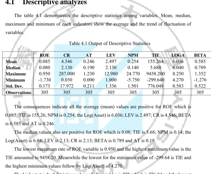
4.1 Descriptive analyzes

The table 4.1 demonstrates the descriptive statistics among variables. Mean, median, maximum and minimum of each indicators show the average and the trend of fluctuation of variables.

Table 4.1 Output of Descriptive Statistics

ROE CR AT LEV NPM TIE LOGA BETA

Mean 0.085 4.546 0.246 2.497 0.254 155.264 6.036 0.585 Median 0.080 2.130 0.190 2.130 0.140 5.680 6.040 0.789 Maximum 0.950 287.000 1.230 12.980 24.770 9458.200 8.250 1.352 Minimum -1.730 0.030 0.000 1.000 -5.750 -299.640 4.270 -1.276 Std. Dev. 0.173 17.972 0.211 1.336 1.501 776.048 0.583 0.522 Observations 305 305 305 305 305 305 305 305

The consequences indicate all the average (mean) values are positive for ROE which is 0.085; TIE is 155.26; NPM is 0.254; the Log(Asset) is 6.036; LEV is 2.497; CR is 4.546; BETA is 0.585 and AT is 0.246.

The median values also are positive for ROE which is 0.08; TIE is 5.68; NPM is 0.14; the Log(Asset) is 6.04; LEV is 2.13; CR is 2.13; BETA is 0.789 and AT is 0.19.

The lowest maximum rate of ROE variable is 0.950 and the highest maximum value is the TIE amounted to 9458.20. Meanwhile the lowest for the minimum value of -299.64 is TIE and the highest minimum values follow by Log(Asset) of 4.270.

The highest standard deviation values of all variables is TIE which is 776.04 and the lowest standard deviation is ROE amounted to 0.173. Thus, based on the results of the descriptive analysis it showed generally all variables has the positive descriptive statistics values.

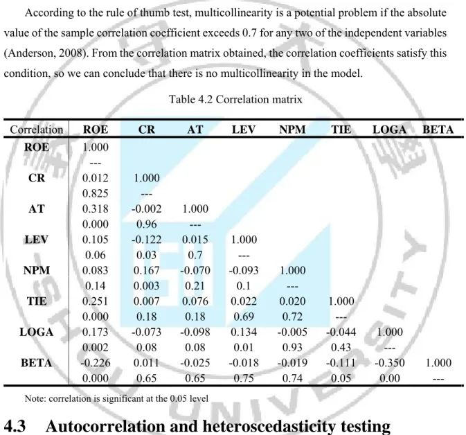
4.2 Correlation test

Pearson correlation is designed to explore whether or not a correlation between two categorical variables and measure the strength and direction of the linear correlation inside the

(32)

two concepts. The Pearson correlation initiates a coefficient was named the Pearson correlation coefficient, which is also called r. The r aimed to perform a line of best match by the data of two variables. It is also used to indicate how those data points are far away from line of best match. Pearson's correlation coefficient value can range from -1 which indicated a perfect negative linear relationship to +1 which proved a perfect positive linear relationship (David Lane, 2003). In details, if the Pearson’s r closer to 1 proving a greater correlation between two variables and if there is one variable changing, another will also change. If the Pearson’s r is negative, there will be a negative correlation which means when one variable score raises, another variable score will drop. If Pearson’s r value equal to 0 (zero), there is no link between two variables.

This research will use Pearson’s Correlation to analyze the relationship between one variable to another variable. Table 4.2 shows the result of Pearson correlation for ROE, CR, TIE, NPM, LEV, LOG(ASSET), AT and BETA. It finds that all variables are correlated to another variable. Table 4.2 also shows that there is a moderate positive linear relationship between ROE and AT (r = 0.318, n = 305, p<0.05). The result also finds that there is a moderate positive linear relationship between ROE and TIE and between ROE and LOG(ASSET) respectively (r = 0.251, n = 305, p<0.05) ; (r = 0.173, n = 305, p<0.05). In contrast, there is moderate negative relationship between ROE and BETA (r = -0.226, n = 305, p<0.05). The result also finds that there is a weak positive relationship between ROE to CR and NPM (r = 0.012, n = 305, p<0.05); (r = 0.083, n = 305, p<0.05) and there is a moderate positive relationship with LEV (r = 0.105, n = 305, p<0.05).

Table 4.2 also shows that there is a weak negative relationship between CR to AT, LEV and LOG(ASSET) (r = -0.002, n = 305, p<0.05) ; (r = -0.122, n = 305, p<0.05); (r = -0.073, n = 305, p<0.05), a weak positive relationship to NPM, TIE and BETA (r = 0.167, n = 305, p<0.05); (r = 0.007, n = 305, p<0.05); (r = 0.011, n = 305, p<0.05).

There is a weak negative relationship between AT to NPM, LOG(ASSET) and BETA (r = -0.07, n = 305, p<0.05) ; (r = -0.098, n = 305, p<0.05); (r = -0.025, n = 305, p<0.05), a weak positive relationship between AT to LEV and TIE (r = 0.015, n = 305, p<0.05), ; (r = 0.076, n = 305, p<0.05).

There is a weak negative relationship between LEV to NPM and BETA (r = -0.09, n = 305, p<0.05); (r = -0.01, n = 305, p<0.05), a weak positive relationship between LEV to TIE and LOG(ASSET) (r = 0.022, n = 305, p<0.05), ; (r = 0.134, n = 305, p<0.05).

(33)

There is a weak negative relationship between NPM to LOG(ASSET) and BETA (r = -0.004, n = 305, p<0.05); (r = -0.01, n = 305, p<0.05), a weak positive relationship between NPM to TIE (r = 0.02, n = 305, p<0.05). There is a weak negative relationship between TIE to LOG(ASSET) and BETA (r = -0.044, n = 305, p<0.05); (r = -0.11, n = 305, p<0.05) and finally there is a moderate negative relationship between LOG(ASSET) and BETA (r = -0.350, n = 305, p<0.05).

According to the rule of thumb test, multicollinearity is a potential problem if the absolute value of the sample correlation coefficient exceeds 0.7 for any two of the independent variables (Anderson, 2008). From the correlation matrix obtained, the correlation coefficients satisfy this condition, so we can conclude that there is no multicollinearity in the model.

Table 4.2 Correlation matrix

Correlation ROE CR AT LEV NPM TIE LOGA BETA

ROE 1.000 --- CR 0.012 1.000 0.825 --- AT 0.318 -0.002 1.000 0.000 0.96 --- LEV 0.105 -0.122 0.015 1.000 0.06 0.03 0.7 --- NPM 0.083 0.167 -0.070 -0.093 1.000 0.14 0.003 0.21 0.1 --- TIE 0.251 0.007 0.076 0.022 0.020 1.000 0.000 0.18 0.18 0.69 0.72 --- LOGA 0.173 -0.073 -0.098 0.134 -0.005 -0.044 1.000 0.002 0.08 0.08 0.01 0.93 0.43 --- BETA -0.226 0.011 -0.025 -0.018 -0.019 -0.111 -0.350 1.000 0.000 0.65 0.65 0.75 0.74 0.05 0.00 --- Note: correlation is significant at the 0.05 level

4.3 Autocorrelation and heteroscedasticity testing

This part shows the result of autocorrelation test and heteroscedasticity test to detect autocorrelation and heteroscedasticity diagnose in this model. By this way, it can be seen that the result of regression is ensured BLUE (Best Linear Unbiased Estimator).

(34)

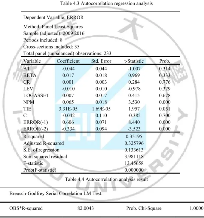
4.3.1 Autocorrelation testing result

To test autocorrelation, firstly, running secondary regression model to test the exist of quadratic autocorrelation in model

(4.1)

Table 4.3 Autocorrelation regression analysis Dependent Variable: ERROR

Method: Panel Least Squares Sample (adjusted): 2009 2016 Periods included: 8

Cross-sections included: 35

Total panel (unbalanced) observations: 233

Variable Coefficient Std. Error t-Statistic Prob.

AT -0.044 0.044 -1.007 0.314 BETA 0.017 0.018 0.969 0.333 CR 0.001 0.003 0.284 0.776 LEV -0.010 0.010 -0.978 0.329 LOGASSET 0.007 0.017 0.415 0.678 NPM 0.065 0.018 3.530 0.000

TIE 3.31E-05 1.69E-05 1.957 0.051

C -0.042 0.110 -0.385 0.700 ERROR(-1) 0.606 0.071 8.440 0.000 ERROR(-2) -0.334 0.094 -3.523 0.000 R-squared 0.35195 Adjusted R-squared 0.325796 S.E. of regression 0.133613

Sum squared residual 3.981118

F-statistic 13.45658

Prob(F-statistic) 0.000000

Table 4.4 Autocorrelation analysis result Breusch-Godfrey Serial Correlation LM Test:

OBS*R-squared 82.0043 Prob. Chi-Square 1.0000

The result indicated that p_value = 1 > α, H0 is accepted that means there is no autocorrelation in this model.

(35)

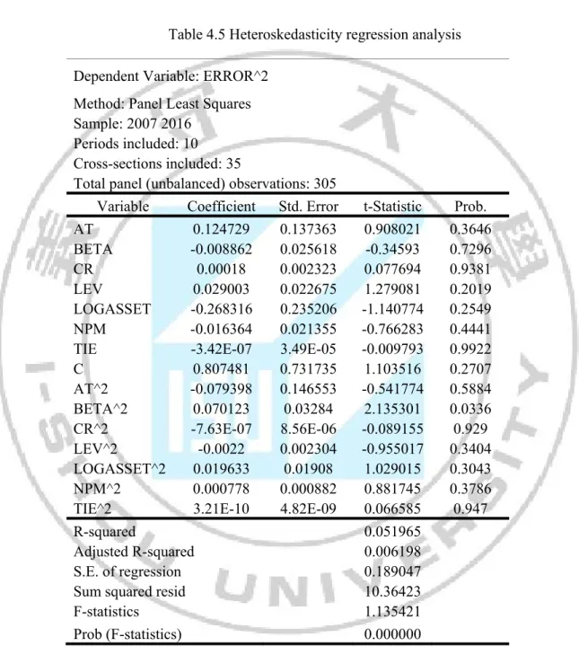
4.3.2 Heteroscedasticity testing result

Run secondary regression model

(4.2)

Table 4.5 Heteroskedasticity regression analysis Dependent Variable: ERROR^2

Method: Panel Least Squares Sample: 2007 2016

Periods included: 10 Cross-sections included: 35

AT 0.124729 0.137363 0.908021 0.3646 BETA -0.008862 0.025618 -0.34593 0.7296 CR 0.00018 0.002323 0.077694 0.9381 LEV 0.029003 0.022675 1.279081 0.2019 LOGASSET -0.268316 0.235206 -1.140774 0.2549 NPM -0.016364 0.021355 -0.766283 0.4441

TIE -3.42E-07 3.49E-05 -0.009793 0.9922

C 0.807481 0.731735 1.103516 0.2707 AT^2 -0.079398 0.146553 -0.541774 0.5884 BETA^2 0.070123 0.03284 2.135301 0.0336 CR^2 -7.63E-07 8.56E-06 -0.089155 0.929 LEV^2 -0.0022 0.002304 -0.955017 0.3404 LOGASSET^2 0.019633 0.01908 1.029015 0.3043 NPM^2 0.000778 0.000882 0.881745 0.3786

TIE^2 3.21E-10 4.82E-09 0.066585 0.947

R-squared 0.051965

Adjusted R-squared 0.006198

S.E. of regression 0.189047

Sum squared resid 10.36423

F-statistics 1.135421

Prob (F-statistics) 0.000000

Table 4.6 Heteroskedasticity analysis result

Heteroskedasticity Test: White

OBS*R-squared 15.8493 Prob. Chi-Square 1.0000 From the result of table 4.6, p_value = 1 > α => Accepted H0 that means there is no heteroskedasticity in this model.

(36)

Therefore, in this model there are no exist of heteroskedasticity, autocorrelation and multicollinearity. It can be seen that the result GLS is BLUE or this model are reliability.

4.4 Regression and hypothesis testing

Regression is the test which analyzes the relationship between variables is negative or positive and the strength of the relationship. To define which model is suitable to analyze this data, Hausman test is conducted and after that regression testing is performed.

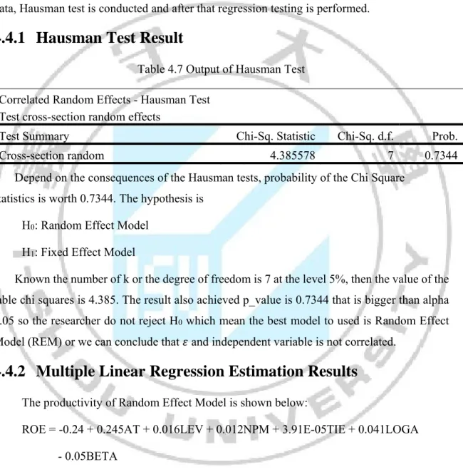
4.4.1 Hausman Test Result

Table 4.7 Output of Hausman Test Correlated Random Effects - Hausman Test

Test cross-section random effects

Test Summary Chi-Sq. Statistic Chi-Sq. d.f. Prob.

Cross-section random 4.385578 7 0.7344

Depend on the consequences of the Hausman tests, probability of the Chi Square statistics is worth 0.7344. The hypothesis is

H0: Random Effect Model H1: Fixed Effect Model

Known the number of k or the degree of freedom is 7 at the level 5%, then the value of the table chi squares is 4.385. The result also achieved p_value is 0.7344 that is bigger than alpha 0.05 so the researcher do not reject H0 which mean the best model to used is Random Effect Model (REM) or we can conclude that and independent variable is not correlated.

4.4.2 Multiple Linear Regression Estimation Results

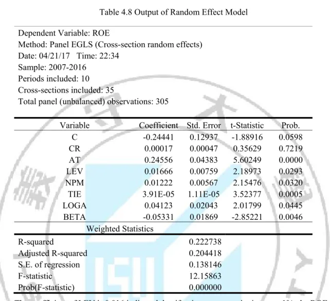
The productivity of Random Effect Model is shown below:

ROE = -0.24 + 0.245AT + 0.016LEV + 0.012NPM + 3.91E-05TIE + 0.041LOGA - 0.05BETA

The results of model testing with Eview 8.1 showed that LOG (ASSETS), AT, NPM, RISK, ATE, TIE variables were statistically significant and these variables accounted for 22.27% of the variation of ROE. Specifically, LOGA (ASSETS), NPM, ATE, TIE and AT have positive associated on the ROE dependent variable, and RISK (BETA) variables have negative associated on ROE changes.

(37)

Table 4.8 Output of Random Effect Model Dependent Variable: ROE

Method: Panel EGLS (Cross-section random effects) Date: 04/21/17 Time: 22:34

Sample: 2007-2016 Periods included: 10 Cross-sections included: 35

C -0.24441 0.12937 -1.88916 0.0598

CR 0.00017 0.00047 0.35629 0.7219

AT 0.24556 0.04383 5.60249 0.0000

LEV 0.01666 0.00759 2.18973 0.0293

NPM 0.01222 0.00567 2.15476 0.0320

TIE 3.91E-05 1.11E-05 3.52377 0.0005

LOGA 0.04123 0.02043 2.01799 0.0445 BETA -0.05331 0.01869 -2.85221 0.0046 Weighted Statistics R-squared 0.222738 Adjusted R-squared 0.204418 S.E. of regression 0.138146 F-statistic 12.15863 Prob(F-statistic) 0.000000

The coefficient of LEV is 0.016 indicated that if ratio asset to equity increase 1%, the ROE will surge 1.6%. The coefficient of NPM is 0.012 indicated that if ratio net profit margin increase 1%, the ROE will increase 1.2%. The coefficient of AT is 0.245 showed that if ratio asset turnover increase 1%, the ROE will increase 24.5%. The coefficient of TIE is 3.91E-05 indicated that if ratio times interest earned increase 1%, the ROE will increase 0.0039%. The coefficient of LOGA is 0.041 indicated that if asset ratio increase 1%, the ROE will increase 4.1%. In contrast, the coefficient of BETA is -0.05 indicated that if ratio Risk increase 1%, the ROE will decrease 5%.

4.4.3 The Results of Coefficient Determination Test (R

2

₎

The result of random effects model (REM) showed that the value of the coefficients determination (R2_{) is 0.222738. Therefore, 22.27% variation or the changing to ROE explained} by the independent variables, which are AT, TIE, LOG(ASSET), NPM, BETA and LEV except

(38)

CR towards real estate companies listed on Ho Chi Minh Stock Exchange. Prob (F-statistic) = 0.0000 < α (0.05) indicates the suitability of the model or the model exists. The p_value of coefficients less than α (0.05) shows that only these variables in the model are statistically significant, explaining well the variability of the ROE at the significance level and the 95% confidence level.

4.4.4 The Results of t-statistics value

The results of current ratio (CR) on the ROE are 0.356297 for t-statistics value while the p-statistics value is 0.7219. The result of the probability is larger compared with the level of α = 5 %. It means partially current ratio have no significant impact on ROE.

The results of leverage (LEV) on the ROE are 2.189749 for t-statistics value while the p-statistics value is 0.0293. The result of the probability is smaller compared with the level of α = 5 %. It means partially leverage have positive significant impact on ROE.

The results of net profit margin (NPM) on the ROE are 2.154763 for t-statistics value while the p-statistics value is 0.0320. The result of the probability is smaller compared with the level of α = 5 %. It means partially net profit margin have positive significant impact on ROE.

The results of asset turnover (AT) on the ROE are 5.602498 for t-statistics value while the p-statistics value is 0.0000. The result of the probability is smaller compared with the level of α = 5 %. It means partially asset turnover have positive significant impact on ROE.

The results of time interest earned (TIE) on the ROE are 3.523776 for t-statistics value while the p-statistics value is 0.0005. The result of the probability is smaller compared with the level of α = 5 %. It means partially time interest earned have positive significant impact on ROE.

The results of Risk (BETA) on the ROE are -2.852211 for t-statistics value while the p-statistics value is 0.0046. The result of the probability is smaller compared with the level of α = 5 %. It means partially Risk have negative significant impact on ROE.

The results of assets (LOGA) on the ROE are 2.017998 for t-statistics value while the p-statistics value is 0.0445. The result of the probability is smaller compared with the level of α = 5 %. It means partially assets have positive significant impact on ROE.

(39)

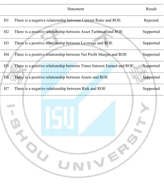
In a summary, the results in table 4.9 show that H1 is rejected and H2, H3, H4, H5, H6 and H7 are all supported.

Table 4.9 Hypothesis Summary

Statement Result H1 There is a negative relationship between Current Ratio and ROE. Rejected

H2 There is a positive relationship between Asset Turnover and ROE Supported H3 There is a positive relationship between Leverage and ROE Supported H4 There is a positive relationship between Net Profit Margin and ROE Supported H5 There is a positive relationship between Times Interest Earned and ROE. Supported H6 There is a positive relationship between Assets and ROE Supported H7 There is a negative relationship between Risk and ROE Supported

(40)

CHAPTER V CONCLUSIONS AND

SUGGESTIONS

5.1 Summary of findings

To achieve research objectives, this study is implemented through several stages and has obtained predetermined objectives. After running the Eview, this study found that 6 hypotheses are supported and one hypothesis is rejected. This study claims the AT, LEV, NPM, RISK, TIE and ASSET affect to ROE of real estate companies listed on HOSE period 2007 - 2016. Meanwhile, AT, LEV, NPM, TIE and ASSET have positively impacted to ROE and RISK has negatively impacted to ROE.

This study found that hypothesis 1 is rejected or current ratio are not significant to ROE ratio. This result goes against the studied literature, besides that research of Pimentel et al. (2005) and Boyed et al. (2007) found that current ratio and profitability has relationship but its profitability is ROA not ROE. My main view for this different result is that the real estate sector may differ from the other previous study analyzed in theories. The operation of the real estate sector goal is long term product such as land, department or house project so profitability is longer achieved than other industry. Current ratio is focused on current liability of company thus it is not related between ROE and current ratio. General research real estate area, Alavinasab & Davoudi (2013), Quan at.el (2015) and Josue (2015) shows that there is no link between ROE and current ratio.

This study found that hypothesis 2 is supported which in line with Boyed et al. (2007), Circiumaru, Siminica and Marcu (2010) and Pouraghajan (2012) who said that there is a positive relationship between ROE and asset turnover. In general, it can be seen that the asset turnover of these companies in that period were not high because the real estate market in 2007 faced many difficulties, many projects were completed but not sold so sales revenue decreased. It had witnessed the global economic crisis in 2008, the real estate market got in trouble, sales of businesses continue to decline. In the period 2010-2013, the real estate market is still underdeveloped, the number of successful transactions reported according to Department of Construction is very low, transaction value is not high, many enterprises accept selling goods hole to rotate the capital. Slow revenue growth is the main reason for the decline in AT rates. Therefore, we can see the serious impact of the financial crisis on the real estate market. Businesses can improve business efficiency by utilizing their available assets to improve AT, therefore to improve ROE, it should focus on increasing Asset Turnover.

(41)

Hypothesis 3 is supported with Boyed et al. (2007). Pagratis et al. (2014) mentioned that also showed that the proportion LEV has positive impact on ROE. Research of Mubin & Hussain (2014), Josue (2015) and equation through DuPont model indicated that the total assets variable explain positive the fluctuations in ROE (Hypothesis 6 supported). This results are suitable of Vietnam economic. In the context of the impact of the global economic crisis in 2008, the State Bank of Vietnam implemented the easing monetary policy which has made the market interest rates decrease but the access to loans still was not easy to all business. In addition, the business situation is not really effective for businesses, so the total assets of the business in spite of increasing, but the growth rate is slower, while customers and investors tend to choose big partners to cooperate. This also affects the performance of real estate firms. In addition, the difficulty of accessing loans is also the reason that the ratio of LEV of enterprises is decreasing, shareholders' equity is much higher than that of loans and enterprises. Therefore, the use of leverage is not effective. Although the impact of LEV and ASSETS to ROE are not strong, but to improve ROE, businesses need to consider improve their ratios.

This study in line of Michell (2001) and Dean (2002) who said that TIE have positive impact to ROE. (H4 supported). Some researchers such as Boyd et al. (2007), Circiumaru et al. (2010); Boldeanu & Pugna (2014) found that relationship between ROE and NPM is positive which means the higher the asset turnover ratio, the greater the profits and the higher the ROE. Nguyen (2015) said that enterprises with NPM are more competitive compared than other partners such as a strong core business, preferential tax policy or low interest rates. The more efficient of business operation, the more profits it will generate in the future because businesses can use these profits to invest instead of borrowing or having trouble of capital scarcity. Profits continue to generate profit, reduced interest burden will help businesses have more motivation to develop. About the condition of Vietnam currently, the access to loans is not easy as it requires procedures, businesses have to go through many stages. Disbursement of the bank takes long times which make business need to wait for capital, therefore the time to implement the project is so long. On the other hand, many real estate businesses have received loans but they do not have an effective business plan that leading revenue is low while interest is coming due. Therefore, if real estate businesses have a rational business strategy, using the loan amount for the right purpose and accumulate profits for reinvestment, it will be a strength to develop in the long term. For that reason, ATE and NPM have same effect on changing of ROE.