Randomized Population with Taguchi’s Method for Multi-objective Optimization

全文

(1)Randomized Population with Taguchi’ s Method for Multi-objective Optimization 1. Cheng-Yuan Tang, 2Yi-Leh Wu, 1Chien-Chin Peng, 1 Chun-Chan Lin, 3Chia-Chen Chen, 3Hsien-Chang Lin 1. 2. Department of Information Management, Huafan University, Taipei, Taiwan, ROC Department of Computer Science and Information Engineering, National Taiwan University of Science and Technology, Taipei, Taiwan 3 Electronics and Optoelectronics Research Laboratories, Hsinchu, Taiwan e-mail: [email protected] ABSTRACT. a selection module, and 3) a variation module as depicted in Figure 1 [14].. Genetic algorithms can be divided into two categories: single objective and multiple objectives. With single objective, we introduce two modified genetic algorithms: the orthogonal genetic algorithm with quantization (OGA/Q), which utilizes the orthogonal design and quantization technique, and the Hybrid Taguchi Genetic Algorithm (HTGA), which utilizes the Taguchi’ s method. Because of the multiple objective functions, the design of the multi-objective genetic algorithms focuses on the fitness assignment, the diversity preservation, and the addition of an elite set. In this paper, we propose to include an additional random population besides the original initial population. In each generation we replace the random population and select only the non-dominated individuals into the elite set. The proposed method can explore more general solution space and can locate better solutions. We then apply Taguchi’ s method to generate better individuals in the additional random population.1 1. INTRODUCTION When the number of variables increases, optimization problems become extremely complex. In the past, people are at a loss how to conquer this kind of problems. With the introduction of the computers, people now can develop effective algorithms and perform simulations on the computers thus make the answer of optimization problems more feasible. For this reason, a number of stochastic search strategies such as evolutionary algorithms, table search, simulated annealing, and ant colony optimization have been developed [14]. Generally speaking, a stochastic search algorithm consists of three parts: 1) a working memory that contains the currently considered solution candidates, 2). 1. This work was supported in part by the National Science Council, Republic of China under Contract No. 94-2213-E-211-012 and 952221-E-011-059.. Figure 1. Components of a general stochastic search algorithm. As to selection, one can distinguish between mating and environmental selection. Mating selection aims at picking promising solutions for variation and usually is performed in a randomized fashion. In contrast, environmental selection determines which of the previously stored solutions and the newly created ones are kept in the internal memory. The variation module takes a set of solutions and systematically or randomly modifies these solutions to generate potentially better solutions. We can divide the evolutionary algorithms into single-objective evolutionary algorithms [4][5][8][10][11][15][18] and multi-objective evolutionary algorithms [6][13][14][16][17] by their number of objective functions. In single-objective evolutionary algorithms, the objective function is the fitness function. Because the number of objective functions in multi-objective evolutionary algorithms is equal or more than two, the fitness functions must have some special arrangements. 2. ORTHOGONAL ARRAY In the whole factor design, when the number of factors increases, the required number of experiments will increase thereupon. Taguchi’ s method utilizes orthogonal array to collect the materials directly, make us obtain more reliable factor result estimator with less experiments. It is an important skill that a robust design utilizes the orthogonal array and carries on the experiments directly. A general orthogonal array is defined as follows:. - 1049 -.

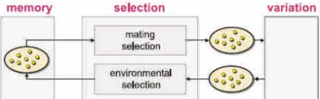
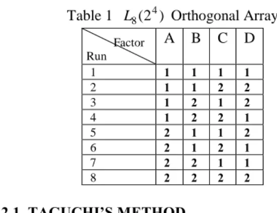
(2) L a (b c ) Where a : number of experiment al runs; b : number of levels for each factor; c : number of columns in the orthogonal array.. An example L8 (2 4 ) orthogonal array is shown in Table 1. Table 1 L8 (2 4 ) Orthogonal Array A B C D Factor Run 1 2 3 4 5 6 7 8. 1 1 1 1 2 2 2 2. 1 1 2 2 1 1 2 2. 1 2 1 2 1 2 1 2. 1 2 2 1 2 1 1 2. 2.1. TAGUCHI’ S METHOD Although Taguchi’ s parameter design method is seldom applied in the field of computer science, it is an important tool for robust design. Taguchi’ s method is often regarded as an engineering methodology to optimize products and process conditions which are minimally sensitive to the causes of variations, and which produce high-quality products with low development and manufacturing costs. Orthogonal array and the SNR (Signal-to-Noise Ratio) are two major tools used in Taguchi’ s method. SNR in Taguchi’ s method is used to assess each level in the contribution degree to the object function of each factor. Formulation of the SNR is derived from the unbiasedness in statistics. It is an estimate of how samples deviate from the center of population. The general formulation of the SNR is as follows: ( y m) S 2. Where y the mean of sample m the mean of object. where p is the number of individuals which can be dominated by X, q is the number of individuals which can dominate X in the objective space, and c is a constant. Following is an example of the dominate relationship:  5  6       3  4    ,  X2  X1  2 3              6  7    .  7  7        5  5     X4  dimension is 4 X3  3 3            5 7      . The definition of dominate is that Xi must be greater than or equal to all X j , with at least one. Xik greater than one X jk . The dominate relationship does not exist in the following example:. 4. THE FUNDAMENTAL MATRIX AND THE EIGHT-POINT ALGOTITHM. S the standard deviation of sample. . 3.2 The Fitness function GPSIFF The fitness assignment strategy is an important issue in solving multi-objective optimization problems. The IMOEA employs the generalized pareto-based scale-independent fitness function (GPSIFF) to quantify the fitness performances in the objective space for both dominated and non-dominated individuals. Let the fitness value of an individual X be a score obtained from all participated individuals by the following function:.    5 5   7  8            3   2 3 5           non - dominate X 6  , X 7  non - dominate X8 dimension is 4 X5  2 2   3    3              5  6 6 5           . 2. SNR 10 log ( y m) 2 S 2. . 3.1 The IGC The IGC[6] uses a divide-and-conquer approach, which consists of three parts: 1. the dividing part: divide large chromosomes into an adaptive number of gene segments; 2. the conquering part: identify potentially good gene segments such that each gene segment can potentially be part of an optimal solution; and 3. the combination part: combine the potentially better gene segments of their parents to produce a potentially good approximation to the best one of all combinations of gene segments.. n 2 ( yi m)   i 1 10 log   n      . . 3. THE INTELLIGENT MULTIOBJECTIVE EVOLUTIONARY ALGORITHM (IMOEA) The IMOEA [6] was proposed by Ho et al. and its purpose is to optimize multiple objective functions simultaneously in order to achieve the optimal solution. In the IMOEA, the Intelligent Gene Collector (IGC) is a main phase and the generalized pareto-based scaleindependent fitness function (GPSIFF) is the fitness assignment strategy.. Given two images in 3D computer vision systems, to establish a general relationship between the two sets of image coordinates which expresses the constraints that the corresponding rays through the two camera centers must intersect in space [1]. When the intrinsic parameters of the cameras are known, the epipolar constraint can be represented algebraically by a 3x3 matrix, called the essential matrix or the fundamental matrix, F. One can compute the fundamental matrix F with the eight-point algorithm stated below. 4.1 The Eight-Point Algorithm. - 1050 -.

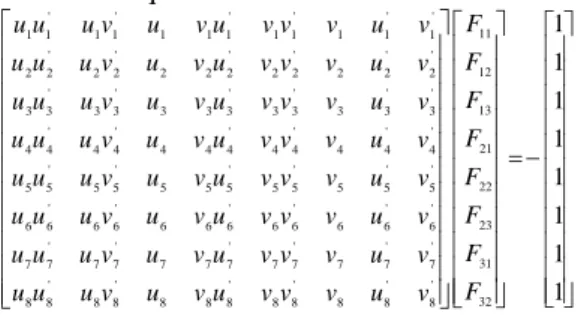
(3) The eight-point algorithm is linear; hence the fundamental matrix F ca be computed fast and easily. The eight-point algorithm for computing the essential matrix was introduced by Longuet-Higgins [1]. The coefficients in the fundamental matrix are in a ninevector which constitutes a linear system.. F11   u , v,1 F21 F  31. u   F13  '  （4-1）  F23  v 0    F33  1   . Compute the disparity (d) of correspondence points. Find the largest and smallest value on X-axis and Y-axis and 1/d of correspondence points, and equally divide them into Q parts.. 3.. Use the orthogonal array LQ 2 Q 3 Q 2 we select. F22 F32. u1v1' u 2 v 2'. u1 u2. v1u1' v 2 u 2'. v1v1' v2 v 2'. v1 v2. u1' u 2'. u 3 v3' u 4 v 4' u 5 v5' u 6 v6'. u3 u4 u5 u6. v3u 3' v 4 u 4' v5 u 5' v6 u 6'. v3 v3' v4 v 4' v5 v5' v6 v6'. v3 v4 v5 v6. u 3' u 4' u 5' u 6'. u 7 v7' u8 v8'. u7 u8. v7 u 7' v8 u 8'. v7 v7' v8 v8'. v7 v8. u 7' u8'. . the Q 2 orthogonal areas.. '. F12. 4.. . Because the coefficients of the fundamental matrix is homogeneous, we therefore decide F33 =1 and let it not zero. Using the eight-points algorithm pi , pi' , i 1,,8 make equation （ 4-1 ） to rewrite the 8×8 linear equation: u1u1'   ' u 2u 2   u 3u 3'  ' u 4u 4   u 5 u 5'  ' u 6u 6   u u' 7 7' u8u 8  . 1. 2.. F11   1 v1'  F   1 v2'  12    ' F13   1 v3     F21   1 v4'    '     1 v5 F22    ' F23   1 v6  F31   1 v7'     F 1 v8'      32  . The great advantage of the eight-point algorithm is that it is linear. If the eight pairs of corresponding points are known, we can compute the parameters of the fundamental matrix. With more than eight points, a linear least squares minimization problem must be solved.. Select eight areas from the Q 2 orthogonal areas and then select one point form each area to form a chromosome.. For example, we first compute the disparity of all correspondence points with Q 3 . We can then divide all correspondence points into 27 areas as shown in Figure 2 and Figure 3. Figure 2 depicts the original date points and Figure 3 depicts the points with added third axis to form the 3-axis bucket.. Figure 2. The 2D coordinates of correspondence points.. 4.2 The Three-Axis Bucket Traditional bucketized algorithms divide the plane into some non-overlapping areas, and then select one point from each area. We propose to use a 3-axis bucket to select points which is distributed over the domain. But in reality, we do not have information about the third axis. When we obtain the 3D models of scenes from two images, the disparity is larger when object is closer to the camera. So we assume that the disparity can be the third axis in our bucket selection scheme. . Given the coordinates of a pair of correspondence points are  x1 , y1 and  x2 , y 2 , we have three ways to compute the disparity of correspondence points, as describes below: x x2  1.  1  y y  2 1. 2 2 2.  x1 x2   y1 y2  3. When the Y-axis values of the correspondence points are the same, we use just  x1 x2  . In this paper, we use the second method above to compute the disparity of correspondence points. The method of selecting correspondence points:. Figure 3. The 3D coordinates of correspondence points in the 3-axis bucket. 5. THE ADDITION OF RANDOM POPULATION After the initial population is generated in IMOEA, all individuals' genes are fixed if there is no mutation operation. When the search space is fixed, we can only find local optima. We propose a new method which includes a randomized population with all individuals is regenerated again with generations. We only include non-dominated individuals in our randomized population to the elite set and exclude other individuals to participate in later evolutions. The proposed method. - 1051 -.

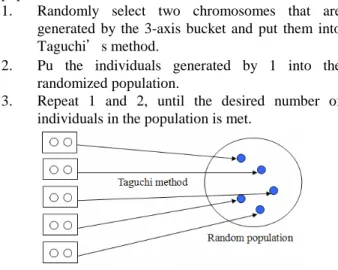
(4) which includes a randomized population can search more feasible solution space and can include better individuals than the ones in the initial population. In The Large Parameter Optimization Problems (LPOPs), individuals in the randomized population are generated in one of the following two ways: 1. Randomly generated individuals: We randomly generate a random population of K individuals, and it is the same way as generating the initial population. 2. Orthogonal quantization generated individuals: It employs the quantization method that originated from the OGA/Q to quantize the domain of every gene, so the individuals can be distributed over the entire domain. We then use Taguchi’ s method to all individuals that are generated by method 1 or 2. Those result individuals are put in the randomized population. In the fundamental matrix optimization problems, individuals in the randomized population are generated in two ways: 1. randomly generates individuals and 2. use 3-axis bucket to generate individuals. We then employ Taguchi’ s method on the result individuals. Those chromosomes that are selected by the above operations have to go through the following operations, as shown below, before include them in the randomized population. 1. Randomly select two chromosomes that are generated by the 3-axis bucket and put them into Taguchi’s method. 2. Pu the individuals generated by 1 into the randomized population. 3. Repeat 1 and 2, until the desired number of individuals in the population is met.. each individual in the populations. Assign each individual a fitness value by using GPSIFF. Update elite sets: add the non-dominated individuals in both the population, random population and e' to e and empty e' . Considering all individuals in e , then remove the dominated ones. If the number NE of non-dominated individuals in e is greater than NEmax, then randomly discard excess individuals Selection: Select Npop-Nps individuals from the population using the binary tournament selection and randomly select N ps. 4.. 5.. individuals from e to form a new population, where N ps N pop  Ps . If. N ps > N ps , let N ps N e . 6.. Recombination: perform the IGC operations for N pop  pc selected parents. For each IGC operation, add non-dominated individuals derived from by-products OA combinations (by-products) and two children to e' . Mutation: apply the conventional mutation operation with PM to the population. Termination test: if a stopping condition is satisfied, stop the algorithm. Otherwise, go to Step 2).. 7. 8.. 6. EXPERIMENTS In this section, we perform experiments that employ the additional random population on top of the IMOEA to solve the Large Parameter Optimization Problems (LPOP) and the estimation of fundamental matrix problems.. Figure 4. Producing population.. individuals. in. randomized. The proposed modification of IMOEA with additional randomized population is described as follows: 1. Initialization: randomly generate an initial population of Npop individuals and create an empty elite set e and an empty temporary elite set e' . 2.. 3.. 6.1 The Large Parameter Optimization Problems While single objective genetic problems can optimize a single function, the multi-objective genetic problem can optimize two or more objective functions in parallel. Our first experiment try to minimize D D 2 and 2 xi 0.5 2xi  10 test functions   xi 10 cos. . i 1. . i 1. together [6], where 5.12 xi 5.12 and D=8.. Randomized population: use the method proposed in section 7.1 to generate K individuals of random population. Evaluation: compute two distances (geometric distance and algebraic distance) and transform them into the fitness values of. - 1052 -. Table 2 LPOP experimental settings. algorithm. IMOEA. IMOEA with Orthogonal random population. IMOEA with Random population. Size of population # of generations. 200. 200. 200. 1000. 1000. 1000. Pc. 0.8. 0.8. 0.8. PM. 0.02. 0.02. 0.02.

(5) fundamental matrix. We want to minimize both functions and together we quantize the performance of the estimated fundamental matrices. In this experiment, Function 1 (F1) is geometric distance and Function 2 (F2) is the algebraic distance. We take the 884 corresponding point pairs (depicted in red as shown in Figure 7) as our experiment data. Table 4 shows the experimental settings.. Table 3 LPOP experiment results. algorithm. IMOEA. IMOEA with Orthogonal random population. IMOEA with Random population. time (in sec). 6554. 9070. 8869. The non-dominated individuals in all experiments are depicted in Figure 5 and Figure 6.. Figure 5. IMOEA(+)、IMOEA+rand. pop.(.) and IMOEA+orthogonal rand. pop.(o) in LPOP.. Figure 7. Corresponding Points.. Table 4. Experimental settings (fundamental matrix estimation). algorithm. IMOEA with 2D bucket. IMOEA with Random population. IMOEA with 3axis bucket and random population. Size of population. 200. 200. 200. # of generations. 500. 500. 500. Pc. 0.8. 0.8. 0.8. PM. 0.02. 0.02. 0.02. # test data points. 884. 884. 884. Figure 6. A zoom in picture of Figure 5. In the LOPO experiments, the original IMOEA, the IMOEA with random population and the IMOEA with orthogonal random population methods can all minimize the two objective functions in parallel. In Figure 6, we show that by adding the randomized population we can find better solutions than the original IMOEA method. And the IMOEA with orthogonal random population outperforms the IMOEA with orthogonal random population method. 6.2 The Fundamental Matrix Optimization Problems We employ the eight-point algorithm to estimate the fundamental matrices with two objective functions. The first function is the geometric distance that measures the distance of all corresponding points to their epipolar lines in image. The second function is the algebraic distance of all corresponding points in the. - 1053 -.

(6) [3]. [4] [5]. [6]. Figure 8. IMOEA+bucket(.)、IMOEA+ rand. pop.(+) and IMOEA+ 3-axis bucket random population (o) – fundamental matrix estimation results. As shown in Figure 8, IMOEA with the randomized population can find better solutions than the original IMOEA and sometimes even outperforms the IMOEA with bucketization. The domain quantization with the orthogonal array method can generate more representative individuals than the pure random generation and the populations are more evenly distributed in the solution domain. However, both the pure random and bucketization can populate more evenly distributed individual in the solution space and the best solutions found by both methods can dominate the solutions generated by the traditional IMOEA. We conclude that by adding the randomized population, we can improve the chance of finding optimal solutions in the IMOEA method. 7. CONCLUSION. REFERENCES. [2]. [8]. [9]. [10]. [11]. [12]. [13]. In this paper, we propose to use an additional randomized population to expand the search space in genetic algorithms to produce better individuals and thus lead to better solutions. The randomized population is not just randomly generated but Taguchi’ s method is also employed to select more representative individuals in the populations. Our experiment results suggest that the proposed method is feasible and can generate better solution than the original IMOEA method. In 2D coordinate system the visual disparity is meaningful. But when we transform the visual disparity into a third axis, how to more evenly distribute the inverse of visual disparity onto the third Z-axis remains an important problem. Our future directions include the use of Principal Component Analysis (PCA) to determine main axis and better quantization on these main axes to locate more diverse corresponding point pairs and eventually lead to better solutions.. [1]. [7]. [14]. [15]. [16]. [17]. [18]. [19]. M.Z.Br o wn,D.Bur s c hka ,a ndG.D.Ha g e r ,“ Adv a nc e s i nCo mput a t i o na lSt e r e o , ”IEEE Trans. Pattern Analysis and Machine Intelligence, Vol. 25, No. 8, Aug. 2003, pp. 993-1008. M.Ca r c a s s o ni ,a nd E.R.Ha nc o c k,“ Co r r e s po nde nc e. - 1054 -. [20]. Ma t c hi ng wi t h Mo da lCl us t e r s , ”IEEE Trans. Pattern Analysis and Machine Intelligence, Vol. 25, No. 12, Dec. 2003, pp. 1609-1615. J .Cha ia nd S.D.Ma ,“ Ro bus tEpi po l a rGe o me t r y Es t i ma t i o n Us i ng Ge ne t i c Al g o r i t hm, ” Pattern Recognition Letters, Vol. 19, 1998, pp. 829-838. L. Davis, Handbook of Genetic Algorithms, Van Nostrand Reinhold, 1996. Y. W.Le ung a nd Y. Wa ng ,“ An Or t ho g o na lGe ne t i c Algorithm with Quantization for Global Numerical Opt i mi z a t i o n, ”IEEE Trans. Evolutionary Computation, Vol.5, Feb. 2001, pp. 41–53. S. Y. Ho , L. S. Shu, a nd J . H. Che n, “ I nt e l l i g e nt Evolutionary Algorithms for Large Parameter Opt i mi z a t i o n Pr o bl e ms , ” IEEE Trans. Evolutionary Computation, Vol.8, No.6, December 2004, pp. 522-541. T. Jones, Evolutionary Algorithms, Fitness Landscapes and Search, Ph.D Dissertation, University of New Mexico, May 1995. J .M.Re nde r sa ndS.P.Fl a s s e ,“ Hy br i dMe t ho dsUs i ng Ge ne t i c Al g o r i t hms f o r Gl o ba lOpt i mi z a t i o n, ” IEEE Trans. Systems, Man, and Cybernetics-part B: Cybernetics, Vol. 26, No. 2, April 1996, pp. 243-258. C.-Y. Tang, H.-L. Chou, Y.-L. Wu and Y.-H. Ding, “ Fa s t and Robust Algorithm Using Coplanar Constraints to Estimate Fundamental Matrices,” IEEE International Conf. Systems, Man and Cybernetics, Taipei, Taiwan, 2006. J. T. Tsai, T. K. Liu, andJ .H.Cho u,“ Hy br i dTa g uc hi Ge ne t i cAl g o r i t hm f o rGl o ba lNume r i c a lOpt i mi z a t i o n, ” IEEE Trans. Evolutionary Computation, Vol. 8, No. 4, Aug. 2004, pp. 365-377. Z.Tua ndY.Lu,“ ARo bus tSt o c ha s t i cGe ne t i cAl g o r i t hm (StGA) for Global Numerical Optimization, ”IEEE Trans. Evolutionary Computation, Vol. 8, No. 5, October 2004, pp. 456-470. W.Zho ng ,J .Li u,M.Xue ,a ndL.J i a o ,“ A Mul t i a g e nt Ge ne t i cAl g o r i t hm f o rGl o ba lNume r i c a lOpt i mi z a t i o n, ” IEEE Trans. Systems, Man, and Cybernetics—part B: Cybernetics, vol. 34, no. 2, April 2004, pp. 1128-1141. Vl a s i sK.Ko umo us i sa ndChr i s t o sP.Ka t s a r a s ;“ A Sa wTooth Genetic Algorithm Combining the Effects of Variable Population Size and Reinitialization to Enhance Pe r f o r ma nc e , ”IEEE Trans. Evolutionary Computation, Vol. 10, No. 1, February 2006. E.Zi t z l e r ,M.La uma nns ,a ndS.Bl e ul e r ,“ A Tut o r i a lo n Ev o l ut i o na r y Mul t i o bj e c t i v e Opt i mi z a t i o n, ” Metaheuristics for Multiobjective Optimization, Lecture Notes in Economics and Mathematical Systems, Springer, vol. 535, 2004, pp. 3–37. Qingfu Zhang and Yiu-Wi ng Le ung , ;“ An Or t ho g o na l Ge ne t i cAl g o r i t hm f o rMul t i me di aMul t i c a s tRo ut i ng , ” IEEE Trans. Evolutionary Computation, Vol. 3, No. 1, Apr 1999 Yimin Liu, Tansel Özyer, Reda Alhajj and Ken Barker “ I nt e g r a t i ng Mul t i -Objective Genetic Algorithm and Validity Analysis for Locating and Ranking Alternative Cl us t e r i ng , ”Informatica 29 (2005) 33–40E. Zi t z l e ra nd L. Thi e l e .“ Mul t i o bj e c t i v ee v o l ut i o na r y algorithms: A comparative case study and the strength pa r e t o a ppr o a c h, ” IEEE Trans. Evolutionary Computation, Vol. 3, No. 4,257–271, 1999. Yueh-Hung Lai, Research on Optimization Using Evolutionary Computation. Master Thesis, Department of Information Management, Huafan University Taipei, Taiwan, May 2005. D. A. Forsyth and J. Ponce. Computer Vision: A Modern Approach. Prentice Hall, 2003. Yan-Hung Ding, 3D Reconstruction of Buildings from Uncalibrated Image Sequences. Master Thesis, Department of Information Management, Huafan University, Taipei, Taiwan, May 2005..

(7)