Data models in geographic information systems

Geographic information systems are

used to collect, analyze, and present

information describing the physical

and logical properties of the

geo-graphic world. Geogeo-graphically

refer-enced data is the spatial data that

pertain to a location on the earth’s surface.

Shashi Shekhar, Mark Coyle, Brajesh Goyal,

Duen-Ren Liu, and Shyamsundar Sarkar

Using object-oriented database technology to model the real world.

Data Models in

Geographic

Information

Systems

geographic information systems (GIS):

• Data Input Unit. Measurements in GIS are taken by sensors such as cameras and global positioning systems. A manual process is then used for inputting data that cannot easily be processed automatically. The measurements are discretized, for example, by imposing a regular, multidimen-sional discrete grid over the surface to be

mea-sured, allowing points of interest to lie only at the intersection of the grid lines. In addition to the error imposed by this discretization process, measurement errors also reduce the accuracy of attribute values. The data input therefore needs validation. Various integrity constraints including topological constraints also need to be checked. An example of a topological constraint is “Min-neapolis should be inside Minnesota.”

data abstraction that hides the details of data storage [9]. It uses logical concepts, which may be easier for most users to understand. It supports data input, manipulation and result presentation. Many GIS are organized as a collection of themes. Each theme represents the values of a unique attribute of the geographic space. A theme may independently partition, decompose, and frag-ment the continuous space for a particular value (or value range) of the attribute. The partitions and fragments of space within each theme are often stored within the database and can be treated as enti-ties or objects. • Data Manipu-lation Capabil-ities. Geographic data is queried and analyzed for various operations, including

spa-tial searches and overlays. Operations on primi-tive vector data-types include geometric operations (e.g., area or boundary, intersection), topological operations (e.g., connectedness) and metric operations (e.g., distance).

• Result Presentation Facilities. A GIS presents results visually (e.g., cartographically) in the form of maps, consisting of graphic images with vector data displayed over raster data; 3D display; ani-mation; and cartographic production. Carto-graphic maps sometimes highlight semantically interesting information at the expense of loca-tional accuracy. This phenomenon is called map generalization.

Related Work and Contribution

The GIS data models can be categorized into

field-based models and object-field-based models. Field-field-based

models see the world as a continuous surface (layer) over which features (e.g., elevation) vary. Layer alge-bra [2] provides a field-based view. It defines a set of operations that can manipulate different layers to produce new layers. The object-based model treats the world as a surface littered with recognizable objects (e.g., cities, mountains, rivers), which exist independent of their locations. GraphDB [7], GODOT [5], Worboy [12], OGIS [3] and GeoOOA [8] are some attempts to model GIS using the object-based approach. OGIS provides a library of spatial types (e.g., point, line, chain) and operations on these types (e.g., intersect, overlap) to facilitate data exchange across different GIS. GeoSAL, Wor-boy and GODOT propose extensive class hierarchies to model the geometry and topology of spatial objects. GraphDB supports the explicit modeling and querying of graphs. GeoOOA adds a geographic dimension to each object modeling a spatial entity, and it supports a fixed set of geometric types and topological relationships. The GERM model [11] attempts to unify the two approaches and provides a set of concepts as an add-on to the ER model for

modeling GIS.

These models do not explicitly support the dis-cretization process and interpolation to invert the discretization. This omission leads to several com-plexities in the existing models, including the dichotomy between field- and object-based approaches.

T

called the Geographic Information Sys-tem Entity Relational model (GISER). This model explicitly represents the discretization aspects so as to unify the two approaches. GISER extends the Enhanced Entity Relationship (EER) model [9] to include con-tinuous fields. The concon-tinuous fields are associated with discretizations and interpolation models.

Data Input Data Modeling Data Manipulation Result Presentation

Data Consistency and Quality Continuous Space

Geometry Topology

Set Operations, Spatial Relationships, Network Analysis

Visual Representation

Constraints, Interpretation Discretization, Interpolation models Points, curves, polygons, etc. Networks, Partitions Topological, Direction, Metric Visualization constraints, Maps

Functional Unit Data Modeling Requirement Examples / Issues

Table 1. Summary of requirements GISER attempts to

support the entire GIS process, from the input of data

mea-sured and discretized to the display of this entity and all the data processing that must be performed.

GISER also uses procedure-valued attributes (e.g., the interpolation model) within the EER model. This is not a major departure, as most modern databases support procedure-valued fields. GISER attempts to support the entire GIS process, from the input of data measured and discretized to the display of this entity and all the data processing that must be per-formed. GISER has distinct identifiable components corresponding to each functional unit.

Data Modeling Requirements

Various requirements of a GIS in relation to each of its functional units will be outlined in an informal manner. Readers are referred to [10] for a more for-mal discussion. Table 1 summarizes the modeling requirements on which this article will focus.

Data Input Unit

Consistency and Quality. The measurement and

dis-cretization process is prone to errors and inaccura-cies. Raw geographic measurement data is often processed and interpreted. It is processed to filter

noise or out-of-range data. Then it is interpreted to fit a domain prototype, and from that, outliers are removed. The results of the analysis of this data needs to be interpreted within the error tolerance of the data.

Discretizing Continuous Space. Geographic

phenom-ena occupy continuous space. However, computers and digital databases can only store and manipulate their discrete approximations. The process of dis-cretization raises the issue of interpolation, which estimates the values at various points to generate a cartographic presentation.

Discretization could either be uniform, that is, independent of the spatial entity that it is modeling (e.g., laying a rectangular grid over a continuous two-dimensional domain), or it could be dependent on it (e.g., a thematic layer [11]). A layer is a map-ping from a domain of non-overlapmap-ping geometric regions to a domain of attribute values. In a simple case, a thematic layer consists of a set of polygons, with each polygon being an area of constant value for an attribute. pc ct ct t t Car: c Truck: t Person: p

jan feb mar

Scatter Glyph Plot month of year 1996 high low med accident severity

ramp meter interval

in seconds

hour of day on 4/1/96 Scatter Plot

Time of the day on 4/1/96 Plot Volume of T raffic month of year 1996 Bar Chart number of traffic congestions

Data Model

Geometry. Geographical entities have geometric

properties that can be modeled by the measure-ments, properties, and relationships of points, lines, angles, and surfaces. Two types of geometric data-types are prevalent: Vector data and Raster data. Vec-tor data include points, lines, and polygons, all of which are representations of the space occupied by real-world entities. Raster data is characterized as an array of points, where each point represents the value of an attribute for a real-world area. Baumann [1] gives a more thorough description of various raster image types.

Topology. Some geographic entities have

topologi-cal properties that are unaltered by elastic deforma-tions. Examples include the connectedness of a region and the connectivity between road intersec-tions via road segments. Primitives are required for representing networks, graphs, and partitions as high-level entities [7]. Partitions are related to net-works in that they associate regions with other regions by relationships such as next or adjacent. It is natural to use a direct construct for networks and partitions, for example, for modeling. Additional discussion of topology in GIS can be found in the Worboy model [12].

Data Manipulation Capabilities

Queries in GIS often involve set operations on the geometric and topological properties of spatial enti-ties. These set operations could be classified into the following groups:

• Spatial selection of a subset from an entity set that fulfills a spatial predicate. Some examples are:

Find all cities in Minnesota, Find all cities no more than 500 miles from Minneapolis.

• Spatial join produces a set of pairs of spatial objects from two layers or entities that satisfies a spatial predicate. For example: For each river, find

all cities within 50 miles.

• Transformation synthesizes a set of layers (a set of spa-tial objects) into a new layer using spatial predi-cates. Some examples are:

Map generalization, trans-formation of vector layer to raster representation.

• Network analysis represents a set of queries on spatial networks, such as route evaluation, network over-lay, and path optimization. Route evaluation is concerned with aggregating attribute data over route-units. A route-unit represents a collection of arcs with common characteristics (e.g., name). A network overlay enables the integration of dis-parate network-attribute databases, which join two or more sets of attributes. Path Optimization models several problems, including shortest path analysis and optimum tour routing.

Queries in GIS use spatial relationships within the query predicates. Spatial relationships can be organized into three categories [6]:

• Topological relationships. These include con-nected, adjacent, inside, and disjoint. These are invariable under topological transformations like translation, scaling, and rotation.

• Direction relationships. These include above, below, or north_of, southwest_of.

• Metric relationships. These include relationships such as the distance between two entities.

Result Presentation Facilities

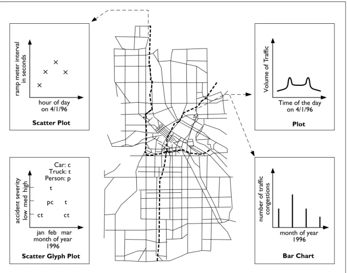
Results in GIS are visually represented in the form of maps, tables, or plots. Visual representation should be able to present all the required information and should not present any information which is not intended. Geographic data is most often displayed on a map. Information on a map is sometimes dis-torted to show some useful feature. For example, the road map in Figure 1 shows each road segment as a straight line. In light of such distortions, maps should be used with caution. Different traffic fea-tures related to the road map are shown using other types of visual representation including a plot, a bar chart, a scatter plot, and a scatter-glyph-plot.

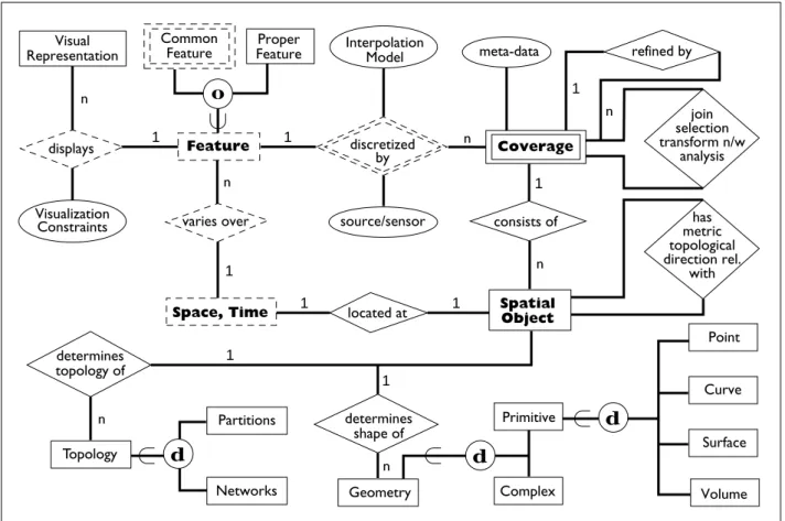
The GISER Data Model

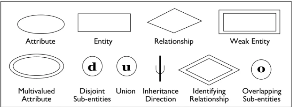
The Geographical Information System Entity Rela-tionship model is shown in Figure 3. It uses the Enhanced Entity Relationship [9] diagram notation

Attribute Multivalued Attribute Disjoint Sub-entities Union Inheritance Direction Identifying Relationship Overlapping Sub-entities Relationship Weak Entity Entity

d

u

o

described in Figure 2, along with dashed lines for continuous fields and relationships. The GISER model is based on four major concepts: Space/Time,

Features, Coverages and Spatial Objects. Space/times

represents boundless multidimensional extents in which geographic phenomena and events can occur and have relative position and direction. It is a con-tinuous field and may possibly be discretized into realms and calendars if needed. Examples of realms include the surface of the earth and its subsets of interest.

Features represent geographic phenomena such as

rivers, vegetation, and cities. GISER models features as continuous fields varying over space and time, thus features as such cannot be stored in a GIS. These must go through the process of discretization in order to compute coverages, which are then stored in a GIS. A feature may have multiple coverages based on multi-ple discretization with varying resolution, accuracy, and sources. A coverage consists of a set of spatial

objects, which occupy a subset of space and time and

have geometric and/or topological properties.

Data Input Unit

Data Consistency and Quality. GISER provides the

relationship refined by to support the data collection

process as well as multiple levels of refinements. GISER states that raw data is refined into processed data, which is refined into interpreted data. Ancil-lary descriptive data, often called meta-data, is pro-vided to facilitate the interpretation and use of the processed data. Meta-data on each coverage would document the refinement procedure and the source.

Continuous Space Modeling. GISER includes

contin-uous fields named features and space/time as well as the relationship discretized by. Each feature represents a mapping from space to a domain of values. Exam-ples of features include elevation, soil type, and water level. Some features are proper features, which represent a collection of uniquely named geographic places such as rivers, cities and countries. Each instance of these entities has a unique name, and the entity’s geographic location can sometimes change. For example, rivers such as the Mississippi flood and change their courses over time. Features that are not proper features are common features, which are identi-fied by their location in space and time and do not have an identification of their own. These entities can be regarded as weak entities that are dependent on and identified by their spatial locations. Exam-ples of common features are land parcels and politi-cal boundaries. Visual Representation Common Feature Proper

Feature Interpolation_Model meta-data refined by

join selection transform n/w analysis has metric topological direction rel. with Point Curve Surface Volume Primitive Complex determines shape of Geometry Partitions Networks determines topology of Topology Feature varies over Space, Time source/sensor located at consists of Spatial Object discretized by Coverage o n n n n n n n 1 1 d d d 1 1 1 1 1 1 1 Visualization Constraints displays

In order to accurately model these entities, GISER makes explicit the fact that continuous entities are dis-cretized for rep-resentation in the database system. Features are discretized to give coverages. There could be multiple cover-ages for the same feature depending on the source/sen-sor. Different interpolation models need to be used for dif-ferent coverages to retrieve a feature.

Specif-ically, GISER includes the relationship discretized by with the attributes interpolation model and source/sensor to model this. A coverage has multiple spatial objects, and is modeled with the relationship

consists of. A spatial object occupies a subset of space

and time, and is modeled using the relationship

located at. Features occupy a subset of space and time

and its attribute takes values defined for a subset of space and time. This is modeled using the relation-ship varies over.

Data Model

Geometry. In the GISER model, geometry is an entity

that is related to a spatial object by the relationship

determines shape of. Additional entities represent the

primitives such as points, lines, and polygons as pro-posed in related models [3, 12].

Topology. Topology is a property belonging to a

spatial object and that property remains unaltered even when the object deforms. An example is a road network. The two nodes in the network thus remain connected even if the path between the nodes is changed by road construction. In order to represent the topology, the basic primitives such as networks (i.e., graphs) and partitions are provided. Additional primitives can be added on lines of the Worboy model [12].

Data Manipulation Capabilities

Spatial relationships are added to the model to accommodate spatial operations in GIS. These rela-tionships include topological relarela-tionships, direction relationships and metric relationships, as described previously. These relationships serve as spatial pred-icates for queries in GIS. Directional relationships involve the location of the objects (examples are north_of, south_of, and northeast_of). Topological relationships involve the regions occupied by the objects (examples are adjacent_to, inside, etc.) Met-ric relationships could involve the geometry and location of the objects (examples include the dis-tance between two objects, or the area of an object that is occupied). To simplify the figure, only the relationships involving spatial objects are kept. A query in GIS is a set operation on one or more cov-erages to give another coverage. This set operation could be join, select, transform or analyze network.

Result Presentation Facilities

GISER proposes that visual representation be speci-fied in the database to declaritively specify the essen-tial properties of the map types. Visual representation consists of primitives such as text,

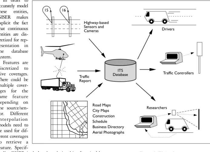
Highway-based Sensors and Cameras Drivers Traffic Controllers Researchers Road Maps City Maps Construction Schedule Business Directory Aerial Photographs Traffic Report ITS Database 15 16

icons, graphs and geometries like points, lines, and polygons. These primitives are associated with a location and orientation inside a visual representa-tion. In addition, visual constraints ensure the visual representation does not convey any information which is not present in the geographic data, and that the visual representation should convey all the infor-mation requested by the user. Visualization con-straints on a road map include: connectivity—that connected road segments should remain connected in the visual representation; and location—that the dis-tortion of the location of various objects should be maintained within acceptable ranges.

Figure 1 shows a few examples of the visual repre-sentation of a road map and of the traffic properties associated with the road map. The representation plot assumes both of the keys are continuous and ordered (e.g., time of the day, volume of traffic at the road segment). The bar chart assumes that one attribute is discrete and that the other is continuous (e.g., month of the year, amount of traffic congestion at the intersection). The scatter plot is a visual repre-sentation of a discrete feature and an ordered discrete feature (e.g., ramp meter interval, hour of the day). The scatter-glyph plot is a visual representation of

two discrete features (e.g., accident severity, month of the year).

An Example GIS Application

Intelligent transportation systems (ITS) are being developed to improve the safety and efficiency of highway travel. Major data sources and users in ITS are shown in Figure 4. Three sources of data are depicted. First, sensors on the highways produce measurements of traffic flow at regular intervals. The road and highway maps represent a second source of data. The traffic reports represent a third source of information to an ITS. Data sent to drivers represents one type of result presentation in an ITS. Vehicles contain graphic display devices that display road maps and current congestions. Traffic controllers at a traffic management center (TMC) may use the data. Also, researchers will often use the data from an ITS for driving simulation to study traffic management and human safety issues.

The GISER Model of the Application

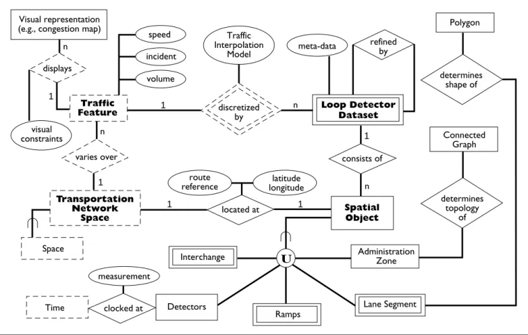
Figure 5 shows a fragment of the GISER data model for a traffic measurement data set. It includes con-tinuous fields (e.g., traffic, visual representation), entities (e.g., loop detector dataset) and relationships

Visual representation (e.g., congestion map)

displays visual constraints Traffic Feature speed incident volume Traffic Interpolation Model meta-data refined by Polygon determines shape of Loop Detector Dataset Connected Graph consists of Spatial Object determines topology of discretized by route

reference longitudelatitude located at varies over Transportation Network Space Space measurement Time clocked at Interchange Detectors Ramps Administration Zone Lane Segment U n n 1 1 n 1 1 1 n 1

(e.g., discretized by, displays). It is based on four major concepts: transportation network space, traffic,

loop-detector dataset and spatial objects. Transportation

network space is a subset of geographic space con-sisting of freeways, highways, and roads. Traffic is the phenomenon of interest in an ITS application, which represents the movements of vehicles and pedestrians over the transportation network space and is characterized by attributes such as speed and volume. The volume of traffic on a road segment refers to the number of vehicles moving across a cross-section. The loop-detector dataset is a set of measurements of the traffic phenomena. The loop detector is a magnetic sensor embedded in the road pavement that measures the volume of traffic. The detectors are linked to the central TMC to collect the traffic measurements over the entire network. The loop detector dataset consists of the traffic mea-surements and the detector locations. Detector loca-tions are classified into area types such as ramps, interchanges and lane segments. Several sensor groupings are of interest, including stations and administration zones. Stations group the detectors on different lanes of a road segment at a milepost. Administrative zones group detectors belonging to common administrative units such as cities or counties.

Data Input Unit. Loop detectors provide

continu-ous analog measurements. A local analog-to-digital converter discretizes the analog readings and accu-mulates them for a specified time period (e.g., 30 seconds). Errors can occur due to bad sensors, out-of-calibration sensors, and communication hazards. This erroneous data needs to be filtered out at mul-tiple levels. At one level, erroneous data may be fil-tered using range checks, parity checks, and similar methods. At another level, it may be removed by

using traffic-flow models and statistical methods. Traffic feature could either be modeled as a proper feature or as a common feature: one instance of a proper feature is aggregate traffic on freeway 35W; one instance of a common feature is aggregate traffic on 35W at mile 5. Measurements from magnetic-loop detectors and cameras represent different cover-ages. Even the transportation network space is discretized by lanes across its width and by road seg-ments across its length. Traffic measureseg-ments at adjacent detectors can also be interpolated over space and time using the traffic flow theory [4].

Data Model. The highways are often represented

in more than one format, since different users of the data have different requirements. One class of users requires that the lane segments, interchanges, and ramps be represented as polygons. Other users work with the topological relationships of the highway network to perform network computations.

Data Manipulation Capabilities. These are the

use-ful aggregate queries for the TMC application. The metric, directional and topological relationships allow queries such as the following:

• Spatial Selection. Show all the incidents on free-ways within 5 miles north of downtown Min-neapolis.

• Spatial Join: Show the intersections of railway lines and roads in Minneapolis.

• Spatial Transformation: Show traffic speeds on all freeway segments. Relative to speed limit, trans-form 80%–100% to green, 60%–80% to yellow, blocked to red, and the remainder to orange. • Network Analysis. Find the shortest path

between two places. Find the shortest path that covers all the road segments to plan removal of snow from all streets.

Result Presentation Facilities. The primary visual

rep-resentation for this application is a road map. A road map can visually show different road types (i.e., one-way, two-one-way, or major roads), by using a different color for each road type. A chosen path can be given a different color from other roads. Multiple attributes of the road (e.g., speed limit, volume) can be shown using different visual attributes of the lines (e.g., color, thickness, shape). As an example, on the freeway map, show road segment as green if traffic is moving at 80%–100% of posted speed, as yellow if at 60%–80%, as red if blocked and all others as orange. Other ancillary visual representations like plots

Future work includes the

evaluation of the GISER model

in different GIS application domains.

and bar charts can also be used, as shown in Figure 1. The plot for the time of the day and the traffic vol-ume is used for identifying rush hours. The bar chart for the amount of traffic congestion and month of the year is used to analyze seasonal variation. The scatter plot for the ramp-meter interval and the hour of the day can be used to correlate ramp-meter rates with traffic volumes for validation of ramp meter rates. The scatter-glyph plot for accident severity and month of the year can be used to analyze seasonal variation in type and frequency of accidents so as to improve safety.

Conclusion

The GISER data model integrates the field-based and object-based models of geographic data by using the discretizes relationship between feature fields and coverage entity. This leads to a simple data model for geographic data like the loop-detector dataset in transportation. Several data management aspects of data input, modeling, query and result presentation can be supported by the simple inte-grated model.

GISER implementation using current relational and object databases raises the issues of implementa-tion of continuous fields (i.e., features). A possible approach is to consider continuous fields to be derived data, which is not physically stored in the database. A procedure to derive continuous fields from various discretizations is assumed. In the con-text of GIS, each coverage has an interpolation model for the discretized feature. Given perfect interpola-tion models, each coverage will lead to the identical continuous field feature. However, given approxi-mate interpolation models, each coverage would yield different estimates of the feature, and these estimates will differ from each other within the mar-gin of error. The meta-data associated with coverage will allow the interpolation of estimated feature val-ues in the context of the approximation errors.

Future work includes the evaluation of the GISER model in different GIS application domains. We would also like to expand the data model to improve the modeling of dynamic and temporal features such as a waterfront. A particular manifestation of the dynamic nature of geographic data occurs in model-ing the boundaries of lakes, oceans, and other natural phenomena. The geometric extent of oceans is dynamic, differing a great deal between low tide and high tide, and therefore presents an interesting challenge.

Acknowledgments

The comments from A. Elhaddi of the National Weather Service, Christiane McCarthy, Siva Ravada, and Andrew Fetterer have greatly improved the read-ability and technical accuracy of this article.

References

1. Baumann, P. Management of multidimensional discrete data. Very Large

Databases Journal 3, 4 (Oct. 1994), 401–444.

2. Delis, V., Hadzilacos, T., and Tryfona, N. An Introduction to Layer

Al-gebra. Tech. Rep. CTI-94.01.2, Computer Technology Institute,

Uni-versity of Patras, Greece, 1994.

3. Draft Base Document-OGIS Project Document 94-025R1. The Open Geodata Interoperability Specification, October 1994.

4. Gerlough, D.L., and Huber, M.J. Traffic Flow Theory: A Monograph.

Spe-cial Report 165. Transportation Research Board National Research

Council, Washington D.C., 1974.

5. Gunther, O., and Riekert, W. The design of GODOT: An object-ori-ented geographical information system. IEEE Data Engineering Bulletin

16, 3 (1993).

6. Guting, R. An introduction to spatial database systems. Very Large

Databases Journal 3, 4 (1994).

7. Guting, R.H. GraphDB: Modeling and querying graphs in databases. In Proceedings of the Int. Conference on Very Large Data Bases (1994). 8. Kosters, G., Pagel, B.U., and Six, H.W. Object-oriented requirements

engineering for GIS applications. In Proceedings of the ACM International

Conference on Geographical Information Systems (1995).

9. Navathe, S.B. Evolution of data modeling for databases. Commun. ACM

35, 9 (Sept. 1992), 112–123.

10. Roman, G. Formal specification of geographic data processing require-ments. IEEE Trans. Knowledge and Data Engineering 2, 4 (Dec. 1990). 11. Tryfona, N., and Hadzilacos, T. Geographic applications development: Models and tools for the conceptual level. In Proceedings of the ACM

In-ternational Conference on Geographical Information System (1995).

12. Worboy, M.F. Object-oriented approaches to geo-referenced informa-tion. Int. J. Geographical Info. Syst. 8, 4 (1994).

Shashi Shekhar ([email protected]) is an associate profes-sor in the Department of Computer Science at the University of Minnesota.

Mark Coyle ([email protected]) is a research scientist at Oracle Corporation.

Brajesh Goyal ([email protected]) is a graduate student at the University of Minnesota.

Duen-Ren Liu ([email protected]) is an assistant professor with the Institute of Information Management at the National Chaio Tung University in Taiwan.

Shyamsundar Sarkar ([email protected]) is a senior member of the research staff at Informix Corporation.

This work was supported by the Federal Highway Authority (FHWA), the Intelligent Transportation Institute (University of Minnesota), Computing Devices International (Minneapolis), and the Minnesota Department of Transportation. Portions of this work was done when S. Sarkar was at the Unisys RDBMS group in Roseville, Minnesota.

Permission to make digital/hard copy of part or all of this work for personal or class-room use is granted without fee provided that copies are not made or distributed for profit or commercial advantage, the copyright notice, the title of the publication and its date appear, and notice is given that copying is by permission of ACM, Inc. To copy otherwise, to republish, to post on servers, or to redistribute to lists requires prior spe-cific permission and/or a fee.

© ACM 0002-0782/97/0400 $3.50