國立交通大學
財務金融研究所
碩 士 論 文
買賣權隱含波動度差與現貨報酬動能:
ETF 選擇權與 ETF 市場分析
An analysis of Implied Volatility Spread and
Underlying Asset Momentum across
ETF Option and ETF market
研 究 生:沈志堅
指導教授:鍾惠民博士 蔡蒔銓博士
買賣權隱含波動度差與現貨報酬動能:
ETF 選擇權與 ETF 市場分析
Analysis of Implied volatility spread and
underlying asset momentum across
ETF Option and ETF market
研 究 生:沈志堅 Student: Chih-Chien Shen
指導教授:鍾惠民博士 Advisor: Dr. Huimin Chung
蔡蒔銓博士 Dr. Shih-Chuan Tsai
國立交通大學
財務金融研究所
碩士論文
A Thesis Submitted to Graduate Institute of Finance
National Chiao Tung University
in partial Fulfillment of the Requirements
for the Degree of Master of
Science in Finance
June 2008
Hsinchu, Taiwan, Republic of China
中華民國九十七年六月
i
買賣權隱含波動度差與現貨報酬動能:
ETF 選擇權與 ETF 市場分析
學生:沈志堅 指導教授:鍾惠民博士
蔡蒔銓博士
國立交通大學財務金融研究所 碩士班
摘 要
本研究主要在探討ETF選擇權價格與ETF現貨報酬動能之間的動態關
係,採用美國S&P 500指數、Nasdaq 100指數及DJIA指數的ETF與ETF選擇
權商品來研究,觀察資訊傳遞在不同的指數類型中有何差異。利用時間序
列模型檢驗ETF選擇權隱含波動度差與ETF過去報酬期間的相關性,以觀察
在ETF選擇權市場中是否存在動能交易的現象,藉此了解ETF選擇權交易者
除了對於未來趨勢的捕捉之外,是否會參考過去ETF現貨市場的績效。另外
比較ETF化與非ETF化的指數選擇權商品,對於動能交易的影響性,以了解
指數的可交易性是否為研究選擇權與現貨市場相關議題時,必須控制的重
要因素。
關鍵詞
動能、選擇權、隱含波動度差、指數股票型基金
An analysis of the implied volatility spread and underlying asset
momentum across ETF Option and ETF market
Student:Chih-Chien Shen Advisor:Dr. Huimin Chung
Dr. Shih-Chuan Tsai
Graduate Institute of Finance
National Chiao Tung University
ABSTRACT
The purpose of this study is to investigate the dynamic relationship between ETF options’ prices and the ETF market momentum. Using the ETF and the ETF option collected from U.S. S&P 500 Index, Nasdaq 100 Index, and DJIA Index, we observe the difference on information transmission among different types of Indices. To examine our thesis, we employ the time-series model to investigate the relation between the implied volatility spreads of ETF options and the returns on ETF during a period. In other words, we observe whether there exists momentum trading in ETF option market and attempt to recognize that whether the traders of ETF options not only chase the market trend but also refer to the ETF performance in the past. Finally we compare the impacts on momentum trading between ETF option and index option to realize that whether the trading practicability of index is the essential factor to control when investigating the related subjects of option market and spot market.
Keywords
iii
誌 謝
困惑、失望、焦急、興奮、快樂,這段撰寫論文之路,走起來是多麼的艱辛漫長, 是如此的百般滋味。猶記三個月前,那辛苦半年的構思全化為泡影,一切需要從頭來過 的挫折,讓我對自己產生了懷疑,感謝瀞云你的支持,你的微笑是我活力的促進劑,因 為有妳,讓我知道我的努力為了什麼而存在,遇見你是我這輩子最甜蜜的事,未來我們 還要一起走下去。感謝蓓華與珮婷,妳們兩姊妹淘時常在一些小地方上幫忙我,與你們 相處在一起依舊能保有學生的純真,有妳們真的很棒。振綱與小田,宅在一起的感覺很 好,一輩子的室友一輩子的朋友,多謝你們在生活上的照料。育維跟阿Sam,跟你們兩 個籃球咖打球真的很快樂,感謝你們約我一起運動,讓我重新想起揮汗的快感。感謝曾 經在課業上幫助過我的同學,建賢、建佑、文誠、秋男,以及所有財金所95級的成員們, 少了你們研究所都不研究所了,另外,高立箴老師與陳煒朋老師的建議與指教,使得論 文能更佳的完善,兩位教授的親和也令我如沐春風,由衷的向你們表達我的謝意。 最後要特別感謝我的兩位指導教授與生我的父母,鐘惠民老師感謝你給予我很大的 揮灑空間,讓我能研究自己喜歡的領域。感謝蔡蒔銓老師,你不厭其煩的回答我的疑惑, 並且常常的為我打氣加油,讓我能夠很有自信的向前走,請保重你的身體,有朝一日, 一定要再跟你小酌一杯敘敘舊。爸、媽,當你們的兒子,是我這輩子幸福的事,感謝你 們當初的意外,這份喜悅與榮耀獻給你們,孩兒不孝,求學的路上常常令你們擔心,但 你們仍不求回報的關心我,並給予我最自由的教育,有你們才有現在的我,將來我一定 會成為你們的驕傲,感謝你們。 志堅 二零零八年七月 謹誌於 新竹交大
-Table of Contents
摘 要 ... i ABSTRACT ... ii List of Tables ... v 1. Introduction ... 1 2. Literature Review ... 62.1 Option Market and Stock Market ... 6
2.2 Price Discovery of ETF ... 9
2.3 Option Prices and Stock Market Momentum ... 10
3. Data and Methodology ... 15
3.1 Data Resources ... 15
3.2 European Options ... 16
3.3 American Options ... 18
3.4. The Weighting Scheme of Implied Volatility ... 20
3.5 Regression of time series ... 24
4. Empirical Result ... 27
4.1. Implied Volatility and the Past Stock Returns of ETF ... 27
4.2 Implied Volatility Smiles ... 33
4-3 ETF Option Prices and Stock Market Momentum ... 34
4.4 Robustness Test ... 40
4.4.1 Vector Autoregression Model (VAR) ... 40
4.4.2 Vega-weighted scheme and elasticity-weighted scheme ... 41
4.4.3 VXO-weighted scheme (the original-formula VIX) ... 41
4.4.4 Dow Jones Industrial Average and DJX market ... 42
4.4.5 Seemingly Unrelated Regression (SUR) ... 43
5. Conclusion ... 51
v
List of Tables
TABLE 3-1 Basic Characters for SPDR, QQQQ, and DIA ... 15
TABLE 3-2 Basic Characters for SPY Option, QQQQ Option, and DIA Option ... 16
Table 3-3 Sample Characteristics of Volatility Spread for SPY Option ... 23
Table 3-4 Sample Characteristics of Volatility Spread for QQQQ Option ... 23
Table 3-3 Sample Characteristics of Volatility Spread for DIA Option ... 24
TABLE 4-1 Implied Volatilities Separated by Call-Puts, Past Stock Returns, ... 29
TABLE 4-2 Implied Volatilities Separated by Call-Puts, Past Stock Returns, ... 30
TABLE 4-3 Implied Volatilities Separated by Call-Puts, Past Stock Returns, ... 31
TABLE 4-4 Implied Volatilities Separated by Call-Puts, Past Stock Returns, ... 32
TABLE 4-5 Regression of Daily Volatility Spread on Past Market Returns for SPY ... 36
TABLE 4-6 Regression of Daily Volatility Spread on Past Market Returns for QQQQ ... 37
TABLE 4-7 Regression of Daily Volatility Spread on Past Market Returns for DIA ... 38
TABLE 4-8 Regression of Daily Volatility Spread on Past Market Returns for SPX ... 39
TABLE 4-9 SUR Regression of Volatility Spread on Past ETF Returns, Historical Volatility, Skewness, and Put-Call Ratio for SPY ... 48
TABLE 4-10 SUR Regression of Volatility Spread on Past ETF Returns, Historical Volatility, Skewness, and Put-Call Ratio for QQQQ ... 49
TABLE 4-11 SUR Regression of Volatility Spread on Past ETF Returns, Historical Volatility, Skewness, and Put-Call Ratio for DIA ... 50
1. Introduction
Exchange Traded Funds, or ETFs, are an investment vehicle traded on stock exchanges, much like stocks or bonds. ETFs are index-based investment products that allow investors to buy or sell shares of entire portfolios of stock in a single security. Moreover, an ETF is a type of investment company whose investment objective is to achieve the same return as a particular market, and is similar to an index fund in that it will primarily invest in the securities of companies that are included in a selected market index, such as the Dow Jones Industrial Average or the S&P 500.
ETFs had their genesis in 1989 with Index Participation Shares, an S&P 500 proxy that traded on the American Stock Exchange and the Philadelphia Stock Exchange. This product, however, was short-lived after a lawsuit by the Chicago Mercantile Exchange was successful in stopping sales in the United States. similar product, Toronto Index Participation Shares, started trading on the Toronto Stock Exchange in 1990. The shares, which tracked the TSE 35 and later the TSE 100 stocks, proved to be popular. The popularity of these products led the American Stock Exchange to try to develop something that would satisfy SEC regulation in the United States.
Standard & Poor's Depository Receipts (SPY) are shares of a family of exchange-traded funds (ETFs) traded in the United States and managed by State Street Global Advisors (SSgA). Informally, they are also known as Spyders or Spiders. The name is an acronym for the first member of the family, the Standard & Poor's Depository Receipts (SPY), the biggest ETF in the U.S., which is designed to track the S&P 500 stock market index. SPDRs were launched by Boston fund manager SSgA in 1992–1993 as the first exchange-traded fund shares still traded in the United States (preceded by the short-lived Index Participation Shares that launched in 1989.) Devised by American Stock Exchange executive Nathan Most, the
2
fund first traded on that market, but has since been listed elsewhere, including the New York Stock Exchange (NYSE).
The Dow Jones Industrial Average (DJIA) is the most widely quoted stock index. World wide media reports constantly quote DJIA updates. It may be the easiest stock index to track, but the entire index was not easy to trade until the Chicago Board of Trade (CBOT) introduced the DJIA futures contracts in October 1997. Then, it have seen the emergence of the exchange-traded fund (ETF), DIAMOND, in January 1998
The NASDAQ-100 Trust Series 1 Exchange-traded fund, sponsored and overseen since March 21, 2007 by Powershares, trades under the ticker NASDAQ: QQQQ. On December 1, 2004, it was moved from the American Stock Exchange where it had the symbol QQQ to the NASDAQ and given the new four letter code QQQQ. It is sometimes referred to as the "Quad Qs," "Cubes," or simply as "the Qs." In 2000 it was the most actively traded security in the United States, but has since dropped to second place after Standard & Poor's Depositary Receipts. On July 17, 2007, the ETF closed above $50 for the first time since early 2001.
2003 year is a turning point for ETF development occurred the mutual fund scandal which was the result of the discovery of illegal late trading and market timing practices on the part of certain hedge fund and mutual fund companies. In U.S, the number of mutual fund investors has approached half the families so that this market is corresponsively mature. However, these illegal trading behaviors got plastered the investor’s confidence deeply.
ETFs generally provide the easy diversification, Buying and selling flexibility, Transparency, low expense ratios, and tax efficiency of index funds, while still maintaining all the features of ordinary stock, such as limit orders, short selling, and options. Because ETFs can be economically acquired, held, and disposed of, some investors invest in ETF shares as a long-term investment for asset allocation purposes, while other investors trade ETF shares
frequently to implement market timing investment strategies. ETFs generally have lower costs than other investment products because most ETFs are not actively managed and because ETFs are insulated from the costs of having to buy and sell securities to accommodate shareholder purchases and redemptions. ETFs typically have lower marketing, distribution and accounting expenses, and most ETFs do not have. ETFs can be bought and sold at current market prices at any time during the trading day, unlike mutual funds and unit investment trusts, which can only be traded at the end of the trading day. As publicly traded securities, their shares can be purchased on margin and sold short, enabling the use of hedging strategies, and traded using stop orders and limit orders, which allow investors to specify the price points at which they are willing to trade. ETFs generally generate relatively low capital gains, because they typically have low turnover of their portfolio securities. While this is an advantage they share with other index funds, their tax efficiency is further enhanced because they do not have to sell securities to meet investor redemptions. ETFs provide an economical way to rebalance portfolio allocations and to "equitize" cash by investing it quickly. An index ETF inherently provides diversification across an entire index. ETFs offer exposure to a diverse variety of markets, including broad-based indexes, broad-based international and country-specific indexes, industry sector-specific indexes, bond indexes, and commodities. ETFs, whether index funds or actively managed, have transparent portfolios and are priced at frequent intervals throughout the trading day.
Although there are many advantages to invest ETFs, it still go along with some risks. When the Portfolio invests in Underlying ETFs, it will indirectly bear its proportionate share of any fees and expenses payable directly by the Underlying ETF. Therefore, the Portfolio will incur higher expenses, many of which may be duplicative. In addition, Underlying ETFs are also subject to the following risks: (i) the market price of an Underlying ETF’s shares may trade above or below its net asset value; (ii) an active trading market for an Underlying ETF’s
4
shares may not develop or be maintained; (iii) the Underlying ETF may employ an investment strategy that utilizes high leverage ratios; (iv) trading of an Underlying ETF’s shares may be halted if the listing exchange’s officials deem such action appropriate, the shares are delisted from the exchange, or the activation of market wide “circuit breakers” (which are tied to large decreases in stock prices) halts stock trading generally; or (v) the Underlying ETF may fail to achieve close correlation with the index that it tracks due to a variety of factors, such as rounding of prices and changes to the index and/or regulatory policies, resulting in the deviating of the Underlying ETF’s returns from that of the index. Some Underlying ETFs may be thinly traded, and the costs associated with respect to purchasing and selling the Underlying ETFs (including the bid-ask spread) will be borne by the Portfolio.
According to capital markets are more free and international, the derivatives which provided low trading cost and high leverage rapidly develop. Especially in options and implied option investment which become the indispensable financial implements, so there are more and more investors to put money into option markets. The option trading includes abounding market information and psychology, thus the issue that the dynamic relationship between option market and spot market is become important. Because of the option market development, ETFs are also listed ETF option, such as SPY option, QQQQ option, and the DIA option. Combining long-term ETF momentum with option price, this study is desirous that whether the ETF returns influence the option price. It implies that people invest the ETF options which are less familiar whether they would care about past performance as mutual funds. In other words, whether inform traders anticipate that the behavior of momentum investors alter their trading behavior to profit from the follower’s expected reaction. Therefore, informed traders buy more the fundamental value ETF and reinforce the trading by positive feedback traders and drive the price above its fundamental option value.
researching contributions in our study. First, although many literatures discuss the issue between ETF and index market or between ETF and index futures market, there is no study investigating between ETF and ETF option market. Option is one of the most important financial implements over the world, therefore investigating between ETF and ETF market is another important issue.
Second, past literatures regularly used index data to discuss the dynamic relationship between spot market and option market. It does not conform to realistic situation for arbitrage or trading index because trading the components of index has much cost and seriously asynchronous trading. Hence, Using index data has doubts for arbitrage theory and relative Price Discovery issues. ETF is the best investment to trading index instead of index data. Also, in our thesis, we adopted SPY and S&P 500 (DIA and DJIA) data to examine the cross momentum trading and to figure out whether the discrepancy caused by tradable character ( ETF and non-ETF).
Third, this study place emphasis on long-term relationship between ETF and ETF option market. We adopt implied volatility spread and past ETF returns to examine the dynamic relation. We would like to chase the more precise trading behavior and figure out how the trading strategy differs from spot market and option market.
The rest of the paper is organized as follows. In section II, we present the related literature. In section III, we describe our methodology which was used to examine the relationship between implied volatility spread and past underlying asset returns. The data selection is also introduced in Section III. Section IV reports the empirical results and robustness test and Section V concludes the paper.
6
2. Literature Review
2.1 Option Market and Stock Market
In discussing the relationship between option market and sock market, the most studies focus on the issue of the Price Discovery. The Price Discovery, meaning when the market accepts new information, investors will make a judgement based on it and trade in financial market by that, then asset would adjust rapidly to its equilibrium price by market mechanism. Namely, from formulation of diffusion of information to investors' interpretation and trading, the course which assets price reach equilibrium in succession can be called the Price Discovery. The Price Discovery is a characteristic of efficient market that causes market price to contain all information sufficiently and immediately. Thus, it accounts for Dominant market and Price lead-lag relationship.
In the Perfect Market, perfect substitute attribute make asset has only one price because when price discrepances come about, the arbitrage opportunity is appeared at once. In other words, under the arbitrage action, there is no lead-lag relationship between stock and option market. In fact, there are several kinds of trading cost in real market and dissimilar market microstructures in different asset markets. Therefore, information transmission is inconsistency making variance of price movement. Besides, in the imperfect market, information might be exposed by trading actions, so any news is implied in a dominant market foremost.
Past evidence on the lead-lag relation between option and stock prices has been almost US based. It is however often conflicting. Early literatures found that stock options lead the underlying stocks. Manaster and Rendleman (1982) adopted 172 stocks with listed options and 805 trading days. They examine close-to-close returns of portfolios based on the relative difference between stock and option prices and find that closing option prices contain
information that is not contained in closing stock prices. However, a serious problem results from the use of closing data, since the Chicago Board Options Exchange (CBOE) closes ten minutes after the close of the stock market. It is possible that the additional information contained in closing option prices merely reflects more recent rather than better information.
Bhattacharya (1987) in order to overcome the three major limitations of MR, namely, (a) daily closing stock and option prices, (b) their non-simultaneity, and (c) the non-consideration of bid/ask spreads for stocks and options, he used the raw data which contains a record for each transaction and another for each bid/ask update for every option series. He compares implied bid/ask stock prices (calculated from call option prices) to actual bid/ask stock prices to calculate arbitrage opportunities. The stock is considered underpriced (overpriced) if the implied bid (ask) is higher (lower) than the actual ask (bid). A simulated trading strategy based on these arbitrage signals indicates that profits are insufficient to cover transaction costs for all intraday holding periods. However, the Manaster and Rendleman (1982) results are confirmed by Bhattacharya’s finding of statistically significant excess returns for overnight holding periods. Bhattacharya’s test design however suffers in that it only detects whether the option market leads the stock market and not vice versa. Although Bhattacharya recognises this as a problem, the reverse simulations are not performed and although he knows the problem, he didn’t resolve all doubts.
Anthony (1988) required two data-selecting criterions. One is that the call option and their underlying common shares are listed contemporaneously for period from January 1, 1982 through June 30, 1983, and the other is that sample firms must be listed on either the New York Stock Exchange (NYSE) or the American Stock Exchange (AMEX). He uses daily data to examine whether trading in one market causes trading in the other. His analysis is based on econometric tests for causality derived from the work of Granger (1969). Anthony concludes that trading in call options leads underlying assets by one day. However, he finds
8
this to be the case for only thirteen firms, whereas stock volume leads option volume for four firms and no unambiguous direction exists for eight firms. Anthony’s results are subject to the same caveats as Manaster and Rendleman due to the non-simultaneity of the closing times for the two markets.
Stephan and Whaley (1990) conceived that the approach must circumvent two major problems of the previous studies. First, transaction-by-transaction data from the stock and option markets are used. Thus, the biases inherent in the non-simultaneity of closing prices in the two markets are avoided. Second, the analysis focuses directly on the lead/lag relation between the intraday price changes in the stock and option markets rather than indirectly through simulating a trading strategy. They examine empirically the intraday price change transformed into implied stock price changes over five-minute intervals and trading volume relations between stocks and options for a sample of firms whose options were actively traded on the CBOE during the first quarter of 1986. They use multi-variable time series regression analysis to estimate the lead/lag relation between the price changes and trading volume in the option and stock markets. Inconsistent with earlier studies, they find that trading in the stock market leads the option market about fifteen to twenty minutes on average both in terms of price changes and trading activity.
Chan, Chung and Johnson (1993) first confirm Stephan and Whaley’s results using data for the same period of analysis and then show their results can be explained as spurious leads induced by infrequent trading of options. Specifically, they show that the stock price lead disappears when the average of the bid and ask prices is used instead of transaction prices. They also show that minimum price variation rules contribute to the documented stock lead because they cause greater discreteness for the trading of options, since stock and option price movements have a non-linear relationship.
investigate both price changes and volume in the two markets, they analyze the price change relationship and the volume relationship separately. Thus, they provides a comprehensive analysis of the interdependence of net trade volume (buyer-initiated trading volume minus seller-initiated trading volume) and quote revisions for actively traded NYSE stocks and their CBOE-traded options.They show that stock net trade volume, but not option net trade volume, predicts contemporaneous and subsequent stock and option quote revisions, suggesting that informed investors initiate trades in the stock market only. On the other hand, option quote revisions, as well as stock quote revisions, predict subsequent quote revisions in the other market.
2.2 Price Discovery of ETF
Because ETF is become more popular since A.D. 1997 , there are not abundant literature on Price Discovery of ETF. Chu, Hsieh and Tse (1999) show in a Vector Error Correction framework that price discovery still takes place on S&P 500 futures. SPDRs only make a small contribution to the common factor, but more than the spot market. Since the study is based on the ETFs’ first year of trading, it is necessary to view these results with some caution. SPDRs only began to exhibit a high-trading volume years later.
Over the March-May 2000 period, Hasbrouck (2003) analyzes the price discovery process using the information share approach of Hasbrouck (1995) for three major U.S. indices. Investors can take positions on the S&P 500 and Nasdaq-100 indices through individual stocks, floor-traded futures contracts, electronically-traded E-mini futures contracts, options or ETFs. The largest informational contributions come from the futures market, with the ETF market playing a minor, though significant role. Interestingly enough, there was no E-mini contract for the S&P MidCap 400 over the sample period and the ETF information share is the most important for this last index.
10
Recent work by Tse, Bandyopadhyay and Shen (2006) shows that although the E-mini DJIA futures contracts dominate price discovery, Diamonds also play a very significant part in the process. Their results for the S&P 500 highlight a contribution of about 49% for the ETF. However, this does not doubt on Hasbrouck’s (2003) results since they are based on floor-based quotes and trades from the AMEX whereas Tse, Bandyopadhyay and Shen use quotes from the ArcaEx Electronic Crossing Network. The anonymous and immediate trading execution obtained on electronic trading platforms may indeed attract informed trading. 2.3 Option Prices and Stock Market Momentum
According to previous literature, we realize the long-term lead-lag relationships in the options and the underlying asset markets have less been investigated compared to the study of Price discovery in short-term. In imperfect markets, option price can be affected by the momentum of the underlying asset through a number of channels (Amin, 2003), such as investors’ expectations about future stock returns, their demand for portfolio insurance, or their attitude toward the higher moments of stock distribution. First, investors’ expectations about future stock return can depend on past stock return. Namely, it means that price movements in the underlying asset market cause price pressures in the options market at a later market, which suggests that a rise in the asset price triggers trading in the options market. This kind of trading behavior is known as momentum trading and is described in the literature extensively by several authors. Delong, Shleifer, Summers, and Waldmann (1990) introduce positive feedback (momentum) traders, who buy when prices rise and sell when prices fall and who may have a variety of incentives for this behavior. These incentives include trend chasing, inability to meet margin call, or portfolio insurance. Inform traders anticipating the behavior of momentum investors alter their trading behavior to profit from the follower’s expected reaction. Therefore, informed traders buy more than what the fundamental value would suggest which reinforces the trading by positive feedback traders and drives the price
above its fundamental value. Lo and Mackinlay (1988) show that the cross-sectional interaction of security returns over time is an important aspect of stock price dynamics. As an example, we document the fact that stock returns are often positively cross-autocorrelation, which reconciles the negative serial dependence in individual security returns with the positive auto correlation in market indexes. Jegadeesh and Timan (1993) constructed trading strategies which buy past winners and sell past losers realize significant abnormal returns over the 1965 to 1989. For example, the strategy they examine in most detail, which select stock based on their past 6-month returns and holds them for 6 months, realizes a compounded excess return of 12.01% per year on average. The returns of the zero-cost winners minus losers portfolio were examined in each of the 36 months following the portfolio formation date. With the exception of the first month, of the first month, this portfolio realizes positive returns in each of the 12 months after the formation date. However, the longer-term performances of these past winners and losers reveal that half of their excess returns in the year following the portfolio formation date dissipate within the following 2 years.
Chan, K. C.’s (1998) contrarian stock selection strategy consists of buying stocks that have been losers and selling short stocks that have been winners. Preached by market practitioners for years, it is still in vogue on Wall Street and La Salle Street. The strategy is formulated on the premise that the stock market overreacts to news, so winners tend to be overvalued and losers undervalued; an investor who exploits this inefficiency gains when stock prices revert to fundamental values. Many investment strategies, such as those based on the price/earnings ratio, or the book/market ratio, can be regarded as variants of this strategy.
Conrad, Kaul, and Nimalendran (1998) also constructed trading strategies buying past winners and selling past losers to realize that momentum trading strategy was profited for short-term period (one month) and long-term period (3-years to 5- years) and reversal trading strategy was profited for medium term (3-month to 1-year).
12
Hong and Stein (1999) recognize momentum traders as those who condition their trades only on past price changed. This simple trading rule, along with a gradual release of information to news watchers allows for both short-term under-reaction and long-term over-reaction. Hence, if past returns are strongly positive, positive autocorrelation suggests that future stock returns will also be greater than average. Investors can exploit this expectation by buying call options on the market index, thereby creating an upward pressure on call prices. Similarly, if past returns are negative, then future stock returns are projected to be below average. Investors can exploit this expectation by buying put options on the market index, creating an upward pressure on put prices. This is cross-market momentum that the option prices depend on the past manifestation of spot market. Additionally, many researcher consider the momentum trading is common phenomenon for all kinds of financial investment. Hence, if past returns are strongly positive, positive autocorrelation suggests that future stock returns will also be greater than average. Investors can exploit this expectation by buying call options on the market index, thereby creating an upward pressure on call prices. Similarly, if past returns are negative, then future stock returns are projected to be below average. Investors can exploit this expectation by buying put options on the market index, creating an upward pressure on put prices. This phenomenon is cross momentum behavior which past performance transfer to option market.
Second, portfolio insurance consideration suggests that the degree to which market participants want exposure to stock prices can depend on recent stock market movement, which then affects the supply and demand for calls and puts. An easy way of changing the exposure to the stock market is by buying call and put options on a stock market index. If, after market prices have risen, an increased number of market participants demand greater exposure to equities, they can purchase call options on a market index, thereby putting upward pressure on call prices. In this case, all prices rise to increase the supply of call writers.
If, after market prices have fallen, an increased number of market participants demand smaller exposure to equities, they can purchase put options on a market index, thereby putting upward pressure on put prices. In this case, put prices rise to increase the supply of put writers.
Third, past stock returns can change investors’ expectations about the higher moments of stock prices. If investors care about higher moments, then their demand for call and put options can change as their expectations about higher moments change, again creating pressures in call and put prices. For example, previous researches in the stock market have found that investors prefer skewness in stock returns. Once again, changes in market momentum can affect the supply and demand for option by changing investor’ skewness in stock returns.
For stock and option market, Tavakkol (2000) conceived that all of these study probe the short-term relationship (intra-day and next day), as they focus on quick information transfers across markets. Even though the autocorrelation and cross-correlation studies in equity markets cover longer periods of time, the long-term lead-lag relationships in options and the underlying asset markets have not been investigated. They use Black’s (1976) model to calculate implied volatilities and the volatility spread at the end of period t is calculated as the difference between the simple average implied volatility of calls and the corresponding average for puts. The one- to 12-month S&P futures returns are used as momentum variable for spot market. They examined the relationship between option market and spot market by OLS estimates of the regressions of volatility spread on lagged spot market returns and indicated prior one-month and three-month returns on S&P future contracts have explanatory power over volatility spreads observed at the end of the period. This means that buying in the asset market over a one- to three-month period is associated with upward pressure on calls and downward pressure on puts. This positive pressure, triggered by long call and short put trades, increases the implied volatility for calls and lowers the implied volatility for puts, thus
14
reducing the volatility spread at the end of the period, and vice versa. Furthermore, the stabilizing effect of feedback trading is also tested in their study. i.e. , whether the activities in the options market are strong enough to cause a reversal in the underlying market. This result supports the reversion hypothesis and the empirical evidence reported for equity market by Jegadeesh an Titman (1993).
Amin, Coval and Seyhun (2004) adopted the Standard and Poor’s 100 Index (also called OEC options) and the market returns are computed using the value-weighted index of NYSE, AMEX, and NASDAQ stocks to investigate the relationship between option market and stock market. At the beginning, they constructed the Boundary Condition Tests Based on Put-Call Parity for American Options. An increase in past stock returns causes the probability of boundary violation to increase and the magnitude of the arbitrage violation is also added. This observation are acknowledged that stock momentum have a significant impact on option market. Next, They formulated a parametric approach instead of the nonparametric boundary condition violations. The parametric measure of the price pressures in option markets is the implied volatility of call and put prices. Implied volatility is computed using the escrowed dividend modification of the binomial model employed in Harvey and Whaley (1992). Similarly, the relationship between option market and stock market are examined. Their finding is like Tavakkol’s result that past returns is the pressure for option prices. In addition, They suggested that standard option pricing model and past returns are independent is not correct and there is no perfect arbitrage activities to reach the equilibrium of market price.
3. Data and Methodology
3.1 Data Resources
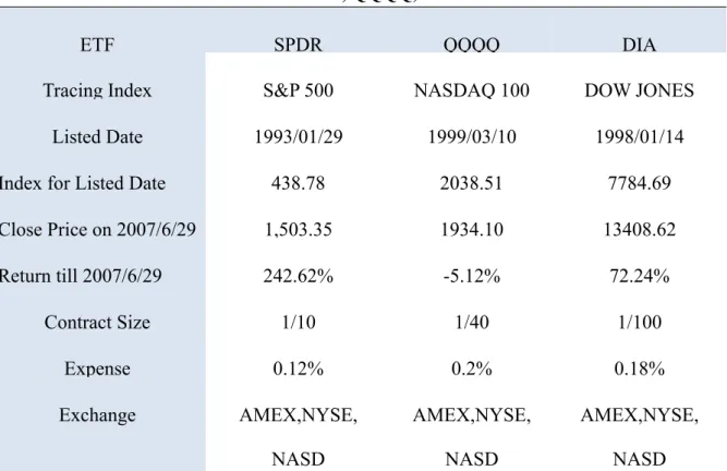
For this study, three of ETFs and SPX index extracted from the Datastream, Bloomberg, and OptionMetrics. Carrying out 2:1 stock split at 2000/03/20 and matching the maximal period of stock return in this study, the QQQQ ETF is collected during 2001/01/02. Past stock return are computed the preceding 10 days (2 weeks), 20days (4 weeks), 30 days (6 weeks), 40 days (8 weeks), 60 days (12 weeks), 80 days (16 weeks), 100 days (20 weeks), 120 days (24 weeks), 150 days (30 weeks), 200 days (40 weeks) of returns as the momentum factor. The deriving data contains the Security ID, its dividends, dividend rate, trading date, close price, open price, bid price, and the ask price. The end of the researching date is 2007/06/29 and Table 3-1 presents other characteristics of underlying asset.
TABLE 3-1 Basic Characters for SPDR, QQQQ, and DIA
ETF SPDR QQQQ DIA
Tracing Index S&P 500 NASDAQ 100 DOW JONES
Listed Date 1993/01/29 1999/03/10 1998/01/14
Index for Listed Date 438.78 2038.51 7784.69
Close Price on 2007/6/29 1,503.35 1934.10 13408.62 Return till 2007/6/29 242.62% -5.12% 72.24% Contract Size 1/10 1/40 1/100 Expense 0.12% 0.2% 0.18% Exchange AMEX,NYSE, NASD AMEX,NYSE, NASD AMEX,NYSE, NASD
New York Stock Exchanges is called NYSE, National Association of Securities Dealers Automated Quotation is called NASD, and American Stock Exchange is call AMEX. The NYSE opened three bigger ETF up to trade on July 31, 2001.
16
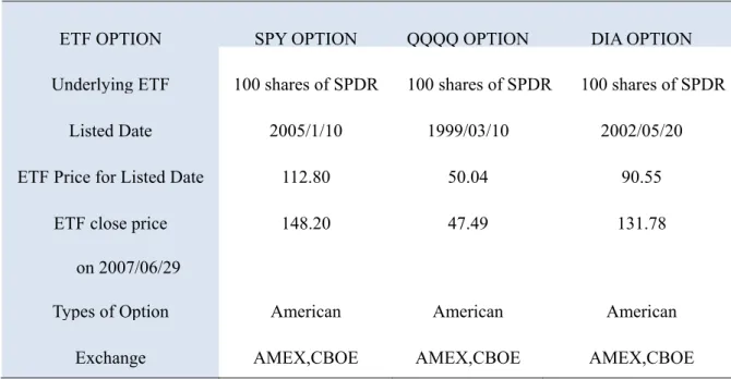
ETF options are provided by the OptionMetrics from 1996/01/02 to 2007/06/29. The categories that we download it contains the option type (call or put), its Security ID, trading date, strike price, expiration date, bid price, ask price, trading volume, implied volatility, and the Greeks. The other attributes of ETF option are described on the Table 3-2.
TABLE 3-2 Basic Characters for SPY Option, QQQQ Option, and DIA Option
ETF OPTION SPY OPTION QQQQ OPTION DIA OPTION Underlying ETF 100 shares of SPDR 100 shares of SPDR 100 shares of SPDR
Listed Date 2005/1/10 1999/03/10 2002/05/20 ETF Price for Listed Date 112.80 50.04 90.55
ETF close price on 2007/06/29
148.20 47.49 131.78
Types of Option American American American Exchange AMEX,CBOE AMEX,CBOE AMEX,CBOE CBOE-Chicago Board Options Exchange
3.2 European Options
The implied volatility spread is considered the barometer of option market, so the first thing we should do is to estimate implied volatility of any sort of option contract. In the OptionMetrics database, Most index options have a European-style exercise feature and can be computed according to the Black-Scholes model (Merton,1973). The Black-Scholes model can be written as ( 1) ( 2) qT rT C=Se− N d −Ke− N d ( 2) ( 1) rT qT P=Ke− N −d −Se− N −d
where 2 1 [ln( / ) ( 1/ 2 ) ]/ , d = S K + − +r q σ T σ T 2 1 / 2 d =d −σ T
C is the price of a call option, P is the price of a put option, S is the current underlying
security price, K is the strike price of the option, T is the time in years remaining to option expiration, r is the continuously-compounded interest rate, q is the continuously- compounded dividend yield, and σ is the implied volatility.
For calculating implied volatilities and associated option sensitivities, the theoretical option price is set equal to the midpoint of the best closing bid price and best closing offer price for the option. The Black-Scholes formula is then inverted using a numerical search technique to calculate the implied volatility for the option. In addition, the interest rate is calculated from a collection of continuously-compounded zero-coupon interest rates at various maturities, collectively referred to as the zero curve. The zero curve used by the option models is derived from BBA LIBOR rates and settlement prices of CME Eurodollar futures. For a given option, the appropriate interest rate input corresponds to the zero-coupon rate that has a maturity equal to the option’s expiration, and is obtained by linearly interpolating between the two closest zero-coupon rates on the zero curve.
The option pricing methodology of the OptionMetrics for equity options assumes that the security’s current dividend yield (defined as the most recently announced dividend payment divided by the most recent closing price for the security) remains constant over the remaining term of the option. This “constant dividend yield” assumption is consistent with most dividend-based equity pricing models (such as the Gordon growth model) under the additional assumptions of constant average security return and a constant earnings growth rate. Even though the dividend yield is constant, this database assumes that the security pays
18
dividends at specific pre-determined times, namely on the security’s regularly scheduled ex-dividend date. In the case of dividends that have already been declared, the ex-dividend dates are known. For dividend payments that are as yet unannounced, the database uses a proprietary extrapolation algorithm to create a set of projected ex-dividend dates according to the security’s usual dividend payment frequency.
3.3 American Options
Options that have an American-style exercise feature are priced using a proprietary pricing algorithm that is based on the industry-standard Cox-Ross-Rubinstein (CRR) binomial tree model. This model can accommodate underlying securities with either discrete dividend payments or a continuous dividend yield.
In the framework of the CRR model, the time between now and option expiration is divided into N sub-periods. Over the course of each sub-period, the security price is assumed to move either “up” or “down”. The size of the security price move is determined by the implied volatility and the size of the sub-period. Specifically, the security price at the end of sub-period i is given by one of the following:
( )
exp 1 up S S u S h i+ = i ≡ i σ(
)
exp 1 down S S d S h i+ = i ≡ i −σWhereh≡T/N is the size of the sub-period, and S
iis the security price at the beginning
of the sub-period. The price of a call option at the beginning of each sub-period is dependent on its price at the end of the sub-period, and is given by:
0 (1 ) / 1 1 max i up down pC p C R i i C i S K ⎧⎡ + − ⎤ ⎫ ⎪⎢⎣ + + ⎥⎦ ⎪ = ⎨ ⎬ ⎪ − ⎪ ⎩ ⎭
and likewise for a put option. Here, r is the interest rate, q is the continuous dividend yield (if the security is an index), R ≡ exp([r-q]h), and Ci+1 and Ci+1 are the price of the option at the end of the sub-period, depending on whether the security price moves “up” or “down”. The “risk-neutral” probability p is given by:
R d p u d − = −
To use the CRR approach to value an option, we start at the current security price S and build a “tree” of all the possible security prices at the end of each sub-period, under the assumption that the security price can move only either up or down
The tree is constructed out to time T (option expiration).
Next the option is priced at expiration by setting the option expiration value equal to the exercise value: C = max(S−K,0) and P = max(K−S,0). The option price at the beginning of each sub-period is determined by the option prices at the end of the sub-period, using the formula above. Working backwards, the calculated price of the option at time i = 0 is the theoretical model price.
To compute the implied volatility of an option given its price, the model is run iteratively with new values of σ until the model price of the option converges to its market price, defined as the midpoint of the option’s best closing bid and best closing offer prices. At this point, the final value of σ is the option’s implied volatility.
20
The CRR model is adapted to securities that pay discrete dividends as follows: When calculating the price of the option from equation (1), the security price S
i used in the
equation is set equal to the original tree price 0 i
S minus the sum of all dividend payments
received between the start of the tree and time i. Under the constant dividend yield assumption, this means that the security price S
i used in equation (1) should be set equal to 0
i
S (1−nδ), where S is the original tree price, δ is the dividend yield, and n is the number i0
of dividend payments received up to time i. All other calculations are the same.
The CRR model usually requires a very large number of sub-periods to achieve good results (typically, N >1000), and this often results in a large computational requirement. The OptionMetrics proprietary pricing algorithm uses advanced techniques to achieve convergence in a fraction of the processing time required by the standard CRR model.
3.4. The Weighting Scheme of Implied Volatility
According to 3-2 and 3-3, we computed implied volatility for every contracts. Each day, for the given set of calls and puts, the implied volatility spread is computed three different ways. The purpose of this exercise is to explore the sensitive of various option to the market momentum hypothesis and ensure that the results are general. The respective weighting schemes are averaging weighted implied volatility (AWIV), vega weighted implied volatility (VGIV), and the elasticity weighted implied volatility (EWIV). We first weight each option implied-volatility equally, averaging across all call and put volatility and taking the difference, resulting in an equally weighted estimate of the implied volatility spread. The concept of AWIV (Trippi, 1977) is that all contracts include the same information and its equation can be written as
1 1 n j j AWIV n = σ =
∑
(3.1) WhereAWIV is the averaging weighted implied volatility, n is the number of
observations, and σj is implied volatility from jth option contract.
Second, we compute vega weighted volatility spread (Latane and Rendleman, 1976). The vega-weighted spread takes a weighted average of all call and put volatilities based on the partial derivative of each option’s price with respect to the volatility. The scheme weights at-the-money options more than out-of-the-money options. If at-the-money options are not affected by market momentum factor, then there should be little or no relation between past stock returns and vega-weighted average spreads. VGIV can be written as
1 1 n j j j j n j j j C VGIV C σ σ σ = = ∂ ∂ = ∂ ∂
∑
∑
(3.2) WhereVGIV is the vega weighted implied volatility, n is the number of
observations, σj is implied volatility from jth option contract, and j j C σ
∂
∂ is the vega value of jth option contract
Our third measure is the elasticity-weighted scheme, which weights by elasticity of each option with respect to the value of the underlying index. This weighting scheme is similar to one used by Chira and Manaster (1978) and incorporates leverage constraints. For example, an investor with limited capital who wishes to gain exposure to directional changes in the stock price typically invests in options with high elasticity. Since the elasticity is decreaing
22
function of how much the option is in the money, this procedure weights out-of-the-money options more than in-the-money options.
1 1 n j j j j j j n j j j j j C C EWIV C C σ σ σ σ σ = = ∂ ∂ = ∂ ∂
∑
∑
(3.3) WhereEWIV is the vega weighted implied volatility, n is the number of
observations, σj is implied volatility from jth option contract, and j j j j C C σ σ ∂ ∂ is the
elasticity of jth option contract.
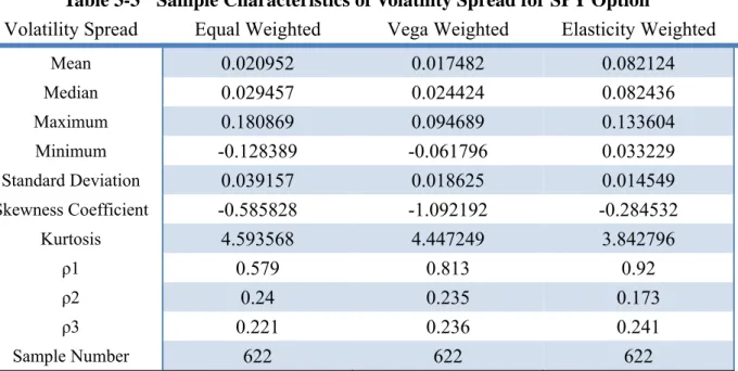
We compute the puts implied volatility and calls implied volatility by formula 3.1, formula 3.2, and formula 3.3 and take the difference so that we can obtain implied volatility spread at any period. Table 3-3, table 3-4, and table 3-5 document the sample statistics for the volatility spread averaged for each trading day for each of the three weighting schemes. Notice that ρ1、ρ2、ρ3 are the partial autocorrelation for average daily volatility spreads. All three series exhibit significantly positive, partial serial correlations. The large, positive first-order autocorrelation suggests that the implied volatility spread follows a slow-moving diffusion process. This finding is again consistent with a situation where the innovation in volatility spread arises from sustained price pressure on either call or put options.
Table 3-3 Sample Characteristics of Volatility Spread for SPY Option
Volatility Spread Equal Weighted Vega Weighted Elasticity Weighted
Mean 0.020952 0.017482 0.082124 Median 0.029457 0.024424 0.082436 Maximum 0.180869 0.094689 0.133604 Minimum -0.128389 -0.061796 0.033229 Standard Deviation 0.039157 0.018625 0.014549 Skewness Coefficient -0.585828 -1.092192 -0.284532 Kurtosis 4.593568 4.447249 3.842796 ρ1 0.579 0.813 0.92 ρ2 0.24 0.235 0.173 ρ3 0.221 0.236 0.241 Sample Number 622 622 622
This table reports summary statistics of the implied volatility spread as a function of type of weighting for SPY option. The volatility spread is computed as the difference between the implied volatility for call options and the implied volatility for put options (put-implied volatility minus call-implied volatility). A single volatility spread is computed each day by weighting the volatility spreads across all option trades in a given day. The terms ρj denote the partial, autocorrelation coefficients of weighted average volatility spreads at daily lag j.
Table 3-4 Sample Characteristics of Volatility Spread for QQQQ Option
Volatility Spread Equal Weighted Vega Weighted Elasticity Weighted
Mean 0.044379 0.026992 0.09855 Median 0.036298 0.026088 0.09647 Maximum 0.42452 0.182499 0.18837 Minimum -0.170715 -0.073992 0.04295 Standard Deviation 0.045795 0.01758 0.02475 Skewness Coefficient 0.97082 1.057694 0.74475 Kurtosis 8.387951 10.08739 3.28697 ρ1 0.09 0.3 0.943 ρ2 -0.023 0.159 0.36 ρ3 0.038 0.165 0.254 Sample Number 1631 1631 1631
This table reports summary statistics of the implied volatility spread as a function of type of weighting for QQQQ option. The volatility spread is computed as the difference between the implied volatility for call options and the implied volatility for put options (put-implied volatility minus call-implied volatility). A single volatility spread is computed each day by weighting the volatility spreads across all option trades in a given day. The terms ρj denote the partial,
24
autocorrelation coefficients of weighted average volatility spreads at daily lag j.
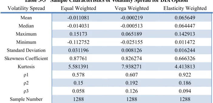
Table 3-3 Sample Characteristics of Volatility Spread for DIA Option
Volatility Spread Equal Weighted Vega Weighted Elasticity Weighted
Mean -0.011081 -0.000219 0.065649 Median -0.014031 -0.000513 0.064447 Maximum 0.15173 0.065189 0.142913 Minimum -0.112752 -0.025155 0.011472 Standard Deviation 0.031196 0.008126 0.016244 Skewness Coefficient 0.87761 0.826274 0.666326 Kurtosis 5.581391 7.938271 4.413813 ρ1 0.578 0.607 0.922 ρ2 0.15 0.192 0.186 ρ3 0.058 0.126 0.094 Sample Number 1288 1288 1288
This table reports summary statistics of the implied volatility spread as a function of type of weighting for DIA option. The volatility spread is computed as the difference between the implied volatility for call options and the implied volatility for put options (put-implied volatility minus call-implied volatility). A single volatility spread is computed each day by weighting the volatility spreads across all option trades in a given day. The terms ρj denote the partial, autocorrelation coefficients of weighted average volatility spreads at daily lag j.
3.5 Regression of time series
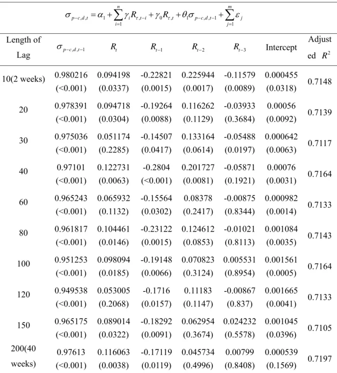
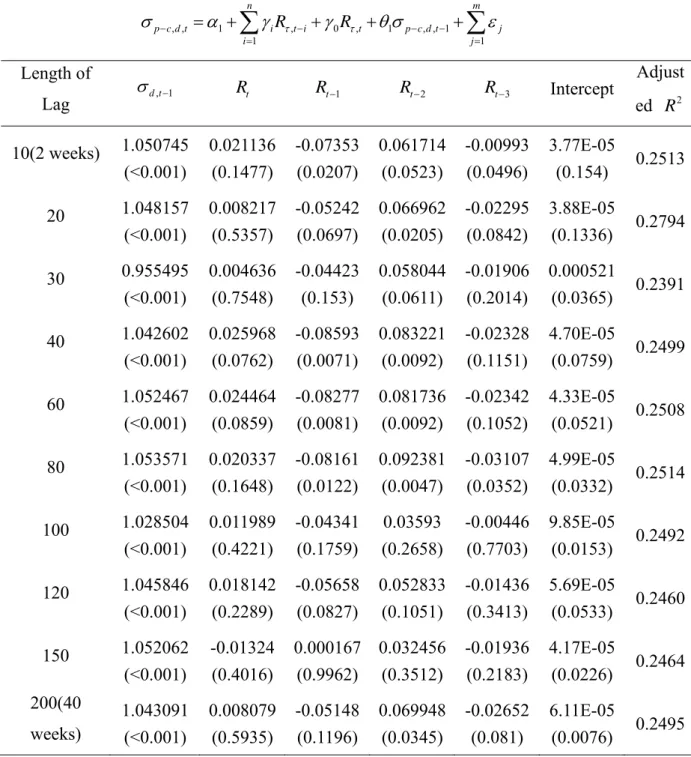
The empirical model we revise and follow by Tavakkol (2000) and Amin et al. (2004) to examine the relationship between past ETF returns and ETF option price. The regression of time series can be estimated and written as
, , 1 , 0 , 1 , , 1 1 n m p c d t i t i t p c d t i j i j Rτ Rτ σ − α γ − γ θ σ − − ε = = = +
∑
+ + +∑
(3.4) where: , , p c d t,t i
Rτ − = The returns on the ETF in the preceding period; ,t
Rτ = The return in the subsequent period (revision); , ,
p c d t i
σ − − = The lagged values of the volatility spread.
τ = The past return period (10, 20, 30, 40, 60, 80, 100, 120, 150, 200 days) The regression equation 3.4 improve Tavakkol’s and Amin’s et al. model. First, the volatility spread in the last trading day of the month and the month returns are used on Tavakkol (2000). It is unreasonable to adopt the option closing price of month computed the implied volatility because the implied volatilities and option price is a continuous time series data. It not only delete too much available sample, but also don’t consider variations daily, even all the sample data was extracted are the negative relationship. Consequently, we use day to day closing data to displace the monthly data
In addition, Tavakkol’s and Amin’s et al. model have another ill-considered problem. They do not revise information was happened on that day. They use a 1-day window between the ending day for computing stock returns and the volatility spread to guarantee that potential investors have the necessary information on hand. However, there is a 15-minute time difference between the closing time of the options market 3:15 PM and the closing time of the underlying futures market 3:00 PM, so it must influence implied volatility spread on subsequent spot market. In order to modify this situation, a variable which was the return in the subsequent period was added to revise new information.
If positive feedback traders of the type described by Delong et al. (1990) use the options markets for their speculative trading, then movements in the options market follow price changes in the underlying asset market. On the other hand, if informed traders use the options market transactions, then the options market would lead the underlying security market. To
26
measure price pressures in the options market we use observed implied volatility in the call and put prices. When there is positive news, speculative traders buy calls and sell puts, which causes a positive pressure in the options market by bidding up the call price and putting downward pressure on put prices. A positive pressure will cause the volatility spread to narrow, and a negative pressure will widen it. If momentum traders use the options market, they buy calls and sell puts when the underlying market rises. When the assets market falls, they sell calls and buy puts. The resulting price pressure would induce a negative relationship between lagged returns in the underlying asset market (Rτ,t i− ) and the volatility spread (
σ
d t, )in the options market at time t. Negativeγ1, thus, supports the notion of momentum trading in
4. Empirical Result
4.1. Implied Volatility and the Past Stock Returns of ETF
Previous studies suggest that the option pricing models systematically misprices option with respect to moneyness and maturity. Short-term options are typically underpriced by Black-Scholes relative to long-term options. Similarly, deep in-the-money and deep out-the-money options are underpriced relative to at-the-money options. Hence, we need to control for option moneyness and maturities examining the relation between implied volatilities and past stock return of ETF.
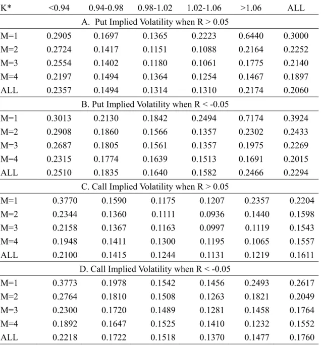
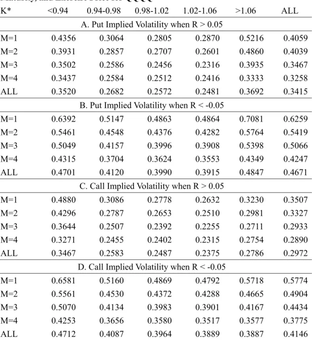
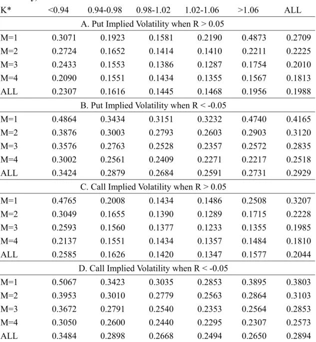
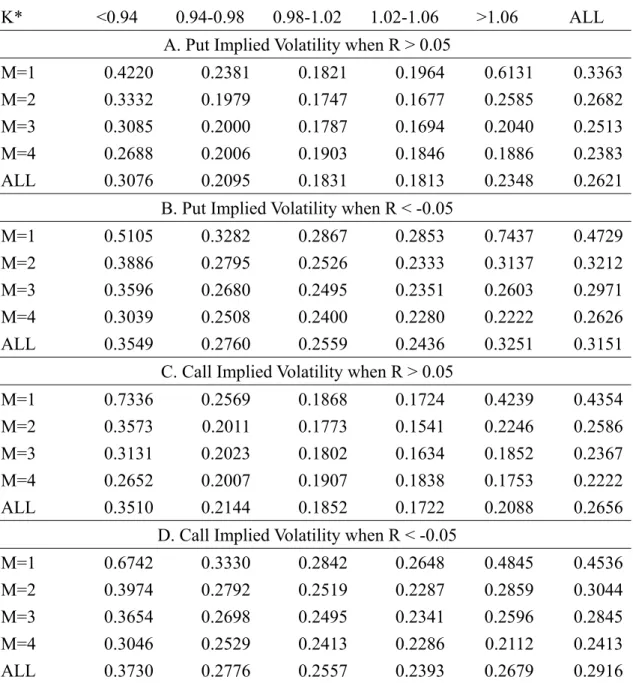
We show the implied volatilities of call and put prices as a function of past 40-day stock returns separated by the strike price and maturity of the options (table 4-1, table 4-2, table 4-3, table 4-4). Table 4-1 is the SPY option, Table 4-2 is the QQQQ option, Table 4-3 is the DIA option, and the Table 4-4 is SPX. Panel A shows the implied put volatilities when past 40-day stock returns are positive (greater than 0.05), and panel B shows the implied put volatility when past stock return are negative (less than -0.05). A decline in stock price increases put-implied volatilities regardless of the maturity and strike price. On average, a switch in returns, from 5% to -5%, increases the put-implied volatilities by about 2.34%, from 20.60% to 22.94% on SPY put option. The QQQQ put increases the implied volatilities by about 12.56%, from 34.15% to 46.71%. The DIA put increases the implied volatilities by about 9.41%, from 29.29% to 9.41%. The SPX put increases the implied volatilities by about 5.3%, from 26.21% to 31.51%. As was mentioned above, the more that the underlying component of ETFs are active, the more implied volatility are affected by past return.
Negative stock returns increase implied volatility estimates across the board, while affecting the short-maturity option(1 month or less), deep-out-of-the-money, and deep-in-the-money options the most. For short-maturity puts, implied volatility of SPY option
28
increases from 30.00% to 39.24%, an increase of 9.24 points; while implied volatility of QQQQ option increases from 40.59% to 62.59%, an increase of 22.00% points ; while implied volatility of DIA option increases from 27.09% to 41.65%, an increase of 14.56 points. as compared with short-maturity option, long–maturity are influenced to a smaller extent.
For call options, the patters are similar (panel C and panel D). A shift from rising to declining stock prices increases put-implied volatilities by 1.49%, from 16.11% to 17.60% on SPY call option. The QQQQ call increases by about 11.74%, from 29.72% to 41.46%. The DIA call increases by about 8.50%, from 20.44% to 28.94%. The SPX call increases by about 3.40%, from 26.56% to 29.16%. All implied volatility estimates increase with declining stock prices. Declines in stock prices increase both call and put option volatilities; however, put-implied volatilities increase more than call-implied volatilities (7.4025 more than 6.285). As a result, put option become relatively more expensive when stock prices decline. Given an increase in stock price, investors bid up the relative prices of call option above those of the put options. Given a decline in stock prices, investors bid up the relative prices of puy options above those of the call options.
TABLE 4-1 Implied Volatilities Separated by Call-Puts, Past Stock Returns, Maturity, and Exercise Price for SPY
K* <0.94 0.94-0.98 0.98-1.02 1.02-1.06 >1.06 ALL
A. Put Implied Volatility when R > 0.05
M=1 0.2905 0.1697 0.1365 0.2223 0.6440 0.3000
M=2 0.2724 0.1417 0.1151 0.1088 0.2164 0.2252
M=3 0.2554 0.1402 0.1180 0.1061 0.1775 0.2140
M=4 0.2197 0.1494 0.1364 0.1254 0.1467 0.1897 ALL 0.2357 0.1494 0.1314 0.1310 0.2174 0.2060
B. Put Implied Volatility when R < -0.05
M=1 0.3013 0.2130 0.1842 0.2494 0.7174 0.3924 M=2 0.2908 0.1860 0.1566 0.1357 0.2302 0.2433 M=3 0.2687 0.1805 0.1561 0.1357 0.1975 0.2269 M=4 0.2315 0.1774 0.1639 0.1513 0.1691 0.2015 ALL 0.2510 0.1835 0.1640 0.1582 0.2466 0.2294
C. Call Implied Volatility when R > 0.05
M=1 0.3770 0.1590 0.1175 0.1207 0.2357 0.2204
M=2 0.2344 0.1360 0.1111 0.0936 0.1440 0.1598
M=3 0.2158 0.1367 0.1163 0.0997 0.1119 0.1543
M=4 0.1948 0.1411 0.1300 0.1195 0.1065 0.1557
ALL 0.2100 0.1415 0.1244 0.1131 0.1219 0.1611
D. Call Implied Volatility when R < -0.05
M=1 0.3773 0.1978 0.1542 0.1456 0.2493 0.2617
M=2 0.2764 0.1810 0.1508 0.1263 0.1821 0.2049
M=3 0.2300 0.1720 0.1489 0.1281 0.1458 0.1764
M=4 0.1892 0.1647 0.1525 0.1410 0.1232 0.1552
ALL 0.2218 0.1722 0.1518 0.1370 0.1477 0.1760
K* represents the standardized exercised price by dividing the exercise price, K, by the value of the ETF at the time of trade. R is the return on the SPY ETF price from day -40 to day -1. All option maturities between day 1 and day 30 are in M = 1, between day 31 and day 60 are in M = 2, between day 61 and day 90 are in M = 3, and greater than 90 days are in M = 4. All implied volatilities are weighted by the number of trades to compute the averages in each cell. Averages across maturities and exercise prices are equally weighted.
30
TABLE 4-2 Implied Volatilities Separated by Call-Puts, Past Stock Returns, Maturity, and Exercise Price for QQQQ
K* <0.94 0.94-0.98 0.98-1.02 1.02-1.06 >1.06 ALL
A. Put Implied Volatility when R > 0.05
M=1 0.4356 0.3064 0.2805 0.2870 0.5216 0.4059
M=2 0.3931 0.2857 0.2707 0.2601 0.4860 0.4039
M=3 0.3502 0.2586 0.2456 0.2316 0.3935 0.3467
M=4 0.3437 0.2584 0.2512 0.2416 0.3333 0.3258
ALL 0.3520 0.2682 0.2572 0.2481 0.3692 0.3415
B. Put Implied Volatility when R < -0.05
M=1 0.6392 0.5147 0.4863 0.4864 0.7081 0.6259
M=2 0.5461 0.4548 0.4376 0.4282 0.5764 0.5419
M=3 0.5049 0.4157 0.3996 0.3908 0.5398 0.5066
M=4 0.4315 0.3704 0.3624 0.3553 0.4349 0.4247
ALL 0.4701 0.4120 0.3990 0.3915 0.4847 0.4671
C. Call Implied Volatility when R > 0.05
M=1 0.4880 0.3086 0.2778 0.2632 0.3230 0.3507
M=2 0.4296 0.2787 0.2653 0.2510 0.2981 0.3327
M=3 0.3644 0.2507 0.2392 0.2255 0.2711 0.2933
M=4 0.3271 0.2455 0.2402 0.2315 0.2754 0.2890
ALL 0.3467 0.2583 0.2487 0.2375 0.2786 0.2972
D. Call Implied Volatility when R < -0.05
M=1 0.6581 0.5160 0.4869 0.4792 0.5718 0.5774
M=2 0.5561 0.4530 0.4372 0.4288 0.4665 0.4904
M=3 0.5070 0.4134 0.3983 0.3901 0.4167 0.4434
M=4 0.4253 0.3656 0.3580 0.3517 0.3577 0.3775
ALL 0.4712 0.4087 0.3964 0.3889 0.3887 0.4146
K* represents the standardized exercised price by dividing the exercise price, K, by the value of the ETF at the time of trade. R is the return on the QQQQ ETF price from day -40 to day -1. All option maturities between day 1 and day 30 are in M = 1, between day 31 and day 60 are in M = 2, between day 61 and day 90 are in M = 3, and greater than 90 days are in M = 4. All implied volatilities are weighted by the number of trades to compute the averages in each cell. Averages across maturities and exercise prices are equally weighted.
TABLE 4-3 Implied Volatilities Separated by Call-Puts, Past Stock Returns, Maturity, and Exercise Price for DIA
K* <0.94 0.94-0.98 0.98-1.02 1.02-1.06 >1.06 ALL
A. Put Implied Volatility when R > 0.05
M=1 0.3071 0.1923 0.1581 0.2190 0.4873 0.2709
M=2 0.2724 0.1652 0.1414 0.1410 0.2211 0.2225
M=3 0.2433 0.1553 0.1386 0.1287 0.1754 0.2010
M=4 0.2090 0.1551 0.1434 0.1355 0.1567 0.1813
ALL 0.2307 0.1616 0.1445 0.1468 0.1956 0.1988
B. Put Implied Volatility when R < -0.05
M=1 0.4864 0.3434 0.3151 0.3232 0.4740 0.4165
M=2 0.3876 0.3003 0.2793 0.2603 0.2903 0.3120
M=3 0.3576 0.2763 0.2528 0.2357 0.2572 0.2835
M=4 0.3002 0.2561 0.2409 0.2271 0.2217 0.2518
ALL 0.3424 0.2879 0.2684 0.2591 0.2731 0.2929
C. Call Implied Volatility when R > 0.05
M=1 0.4765 0.2008 0.1434 0.1486 0.2508 0.3207
M=2 0.3049 0.1655 0.1390 0.1289 0.1715 0.2228
M=3 0.2593 0.1560 0.1377 0.1233 0.1355 0.1985
M=4 0.2137 0.1551 0.1434 0.1357 0.1484 0.1810
ALL 0.2585 0.1626 0.1420 0.1347 0.1577 0.2044
D. Call Implied Volatility when R < -0.05
M=1 0.5067 0.3423 0.3035 0.2853 0.3895 0.3803
M=2 0.3953 0.3010 0.2779 0.2563 0.2864 0.3103
M=3 0.3672 0.2791 0.2540 0.2353 0.2564 0.2853
M=4 0.3050 0.2600 0.2440 0.2295 0.2307 0.2573
ALL 0.3484 0.2898 0.2668 0.2494 0.2650 0.2894
K* represents the standardized exercised price by dividing the exercise price, K, by the value of the ETF at the time of trade. R is the return on the DIA ETF price from day -40 to day -1. All option maturities between day 1 and day 30 are in M = 1, between day 31 and day 60 are in M = 2, between day 61 and day 90 are in M = 3, and greater than 90 days are in M = 4. All implied volatilities are weighted by the number of trades to compute the averages in each cell. Averages across maturities and exercise prices are equally weighted.
32
TABLE 4-4 Implied Volatilities Separated by Call-Puts, Past Stock Returns, Maturity, and Exercise Price for SPX
K* <0.94 0.94-0.98 0.98-1.02 1.02-1.06 >1.06 ALL
A. Put Implied Volatility when R > 0.05
M=1 0.4220 0.2381 0.1821 0.1964 0.6131 0.3363
M=2 0.3332 0.1979 0.1747 0.1677 0.2585 0.2682
M=3 0.3085 0.2000 0.1787 0.1694 0.2040 0.2513
M=4 0.2688 0.2006 0.1903 0.1846 0.1886 0.2383
ALL 0.3076 0.2095 0.1831 0.1813 0.2348 0.2621
B. Put Implied Volatility when R < -0.05
M=1 0.5105 0.3282 0.2867 0.2853 0.7437 0.4729
M=2 0.3886 0.2795 0.2526 0.2333 0.3137 0.3212
M=3 0.3596 0.2680 0.2495 0.2351 0.2603 0.2971
M=4 0.3039 0.2508 0.2400 0.2280 0.2222 0.2626
ALL 0.3549 0.2760 0.2559 0.2436 0.3251 0.3151
C. Call Implied Volatility when R > 0.05
M=1 0.7336 0.2569 0.1868 0.1724 0.4239 0.4354
M=2 0.3573 0.2011 0.1773 0.1541 0.2246 0.2586
M=3 0.3131 0.2023 0.1802 0.1634 0.1852 0.2367
M=4 0.2652 0.2007 0.1907 0.1838 0.1753 0.2222
ALL 0.3510 0.2144 0.1852 0.1722 0.2088 0.2656
D. Call Implied Volatility when R < -0.05
M=1 0.6742 0.3330 0.2842 0.2648 0.4845 0.4536
M=2 0.3974 0.2792 0.2519 0.2287 0.2859 0.3044
M=3 0.3654 0.2698 0.2495 0.2341 0.2596 0.2845
M=4 0.3046 0.2529 0.2413 0.2286 0.2112 0.2413
ALL 0.3730 0.2776 0.2557 0.2393 0.2679 0.2916
K* represents the standardized exercised price by dividing the exercise price, K, by the value of the ETF at the time of trade. R is the return on the SPX ETF price from day -40 to day -1. All option maturities between day 1 and day 30 are in M = 1, between day 31 and day 60 are in M = 2, between day 61 and day 90 are in M = 3, and greater than 90 days are in M = 4. All implied volatilities are weighted by the number of trades to compute the averages in each cell. Averages across maturities and exercise prices are equally weighted.
4.2 Implied Volatility Smiles
Volatility smile refers to the U-shaped implied volatility estimates as a function of the exercise price. Previous option pricing studies have shown that both in-the-money and
out-the-money calls and puts have higher implied volatilities than at-the money calls and puts. Moreover, short-maturity options, deep-in-the money calls, and deep-out-of-money puts have the highest estimated implied volatilities, giving rise to a skew-shaped implied volatility. We document a similar relation in table 4-1, table 4-2, table 4-3, and table 4-4. For the puts of ETF, Three ETF and SPX are existed implied volatility smiles whether past stock return are positive or negative. Furthermore, volatility smiles curve moved upward when the decline of stock prices increases volatility for puts . As observed in table 4-1, implied volatility of SPY put increases from 23.57% to 25.10% for out-the-money puts, increasing from 13.14% to 16.40% for at-the-money puts, and increasing from 21.74% to 24.66% for in-the-money puts.
For in-the-money puts, volatility smiles measure is 12.43% ( 25.57% minus 13.14% ) when past stock return are positive. For out-the-money puts, volatility smiles measure is 8.60% ( 21.74% minus 13.14% ). Also, For in-the-money puts, volatility smiles measure is 8.70% ( 25.10% minus 16.40% ) when past stock return are positive. For out-the-money puts, volatility smiles measure is 8.26% ( 24,66% minus 16.40% ).