依據混合式火箭實驗模型以數值模擬分析其燃燒引擎的燃燒推進過程的研究

(1)

國立交通大學

機械工程學系

碩士論文

CFD Simulation on Model of the Experimental

Hybrid-Rocket Motor

依據混合式火箭實驗模型以數值模擬分析其

燃燒引擎的燃燒推進過程的研究

指導教授：吳宗信博士

研究生：林俊傑

中華民國九十八年七月

(2)

依據混合式火箭實驗模型以數值模擬分析其

燃燒引擎的燃燒推進過程的研究

CFD Simulation on Model of the Experimental

Hybrid-Rocket Motor

研究生

研究生：

：

：林俊傑

林俊傑

Student: Jyun-Jie Lin

指導教授

指導教授：

：

：吳宗信博士

吳宗信博士

Advisor: Dr. Jong-Shinn Wu

國立交通大學

機械工程學系

碩士論文

A Thesis

Submitted to Department of Mechanical Engineering

National Chiao Tung University

in Partial Fulfillment of the Requirements

for the Degree of

Master of Science

In

Mechanical Engineering

July 2009

Hsinchu, Taiwan

2009 年七月

(3)

學生：林俊傑指導教授：吳宗信博士國立交通大學機械工程學系摘要摘要摘要摘要混合式火箭由液態或氣態的氧化劑以及固態燃料組成，與固態以及液態火箭比較下，混合式火箭有以下幾個優點： 1.安全性 2.對於裂縫以及缺陷處的敏感度較低，不會過度燃燒 3.可依賴性 4.能量的控制性 5.多用途燃料 6.設計可改變的空間較大 7.環保 8.花費較低。混合式火箭還是有一些缺點：1.低燃料燃燒效率 2.低體積填充速率 3.燃料在燃燒過後需殘留以防止燒到管壁 4.氧化劑以及燃料的混合比例在燃燒過程中不斷變化 5.混合以及燃燒效率較低。但由於混合式火箭所具有的安全性，低花費以及設計可改變的空間較大，很適合用來做學術研究。在交大吳宗信老師的 APPL 實驗室中，混合式火箭分為實驗組和模擬組，而我負責模擬實驗組設計火箭的燃燒式推進並分析結果。數值模擬中，使用由太空中心的陳彥升博士及其同僚發展出來的 UNIC 軟體來模擬，至於模擬的目標，由於混合式火箭的燃燒效率和推力較低，需改善這兩個項目，模擬的部分分為一開始分別以以 C4H6 和 N2O 為燃料和氧化劑先完成一個基本模型，之後改變入口噴嘴的面積比、火箭燃燒室預熱區尺寸改變、內部燃料

(4)

管道直徑改變、氧化劑質量流率改變以及入口噴入區域形狀改變，最後分析及比較其結果。

從實驗以及模擬結果來看，由太空中心陳博士所設計的新型燃燒室氧化劑噴嘴相當的實用，其可使噴嘴週遭區域在低溫狀態，實際測試幾次後無損壞並可重複使用，並且可平順地將氧化劑導入預熱區和燃料管道中。

(5)

Student: Jyun-Jie Lin Advisor: Dr. Jong-Shinn Wu Department of Mechanical Engineering

National Chiao Tung University

ABSTRACT

Hybrid-Rocket is composed by gaseous or liquid oxidizer and solid fuel. Unlike with Solid and Liquid fuel, Hybrid-Rocket has these advantages: 1.Safety 2. Insensitivity to cracks and imperfections 3.Reliability 4.Energy management 5.Fuel versatility 6.Design flexibility 7.Environmental friendliness 8.Low cost. Of course it has disadvantages like: 1.Slow regression rate 2.Low volumetric loading 3.Fuel residuals 4.Mixture ratio shift 5.Mixing/combustion inefficiencies.

And because of its safety, low cost and Design flexibility, hybrid rocket is suitable for academic research.

In Dr. Wu’s APPL Lab, Hybrid-Rocket research is separated into two groups, the experimental group and simulation group. And I’m in charge of the Hybrid-Rocket combustion CFD simulation, based on the model of experimental group.

In the simulation, we used the simulation code “UNIC” made by Dr. Chen and his colleagues in NSPO. As for our goal, mixing ratio and thrust of Hybrid-Rocket is smaller, so they are the main factors to improve. We used C4H6 and N2O as fuel and oxidizer to finish the basic model. Then, based on this model, we changed the

(6)

simulation conditions area ratio of pintle injector, port size, pre-combustion chamber size, inlet mass flow rate of oxidizer and inlet region geometry. Then we compared the results with the basic model.

From the experimental results, we can see the pintle injector designed by Dr. Chen is quite useful. It maintains a low Temperature region near the pintle injector and thus the pintle injector can be reused for many times without any damage. It can also direct the oxidizer flow well into pre-combustion and fuel port region.

(7)

誌謝

首先感謝我的家人，在我的求學道路上一路支持下去，現在才得以完

成碩士班的學位。接著在碩士班的兩年中，特別感謝吳宗信老師的教

導，在每一次的報告中，總是很有耐心的聽著報告內容，並且在之後

提出不足和需要改進的部分，遇到我沒辦法立刻理解的情況，

吳老師會不厭其煩重複地教導，直到了解為止，我很榮幸能在此實驗

室待這兩年，吳老師對於當前的科技發展狀況一直都有很特別獨到的

見解，讓我受益良多。

另外，也要特別感謝林昆模學長，在接下公司的案子時，不斷的教

導我做投影片的技巧、報告方式以及如何處理廠商要求的進對應退技

巧；感謝 Aziz 在我心煩時會和我聊天，交流台灣和法國的文化，並

且抒發 Aziz 有趣的思想。

感謝 APPL 實驗室提供足夠的資源，讓我能在研究所兩年的時間裡

對於研究的資源充足。

感謝鄭凱文、李允民、洪捷粲、邱老大、江明鴻、胡孟樺、林雅茹、

林昆模、盧勁全、林宗漢、洪維呈等諸位學長姐，感謝他們不厭其煩

的為我在研究以及其他方面解惑。感謝王穎志、古必任以及林逸民諸

位同學，感謝有你們和我一起在研究上互相勉勵和進步。感謝周子

(8)

豪、吳尚穎、呂其璋、黃皓遠諸位學弟、前助理于恩以及現任助理王

姐，感謝你們在各方面的協助。感謝 Hadley、Matt，感謝你們使我

的英文溝通能力和國際觀有所提升。

最後要感謝交大，從大學部一路升上來，學校在許多方面提供了很

多方便的資源，尤其是交大浩然圖書館在各領域充足的館藏，讓我能

夠學到許多領域的知識。

(9)

List of Tables

Table 4.1 Data of the basic model...38

Table 4.2 Data comparison between different area ratios ...38

Table 4.3 Data comparison between different chamber sizes ...39

Table 4.4 Data comparison between different port sizes ...39

Table 4.5 Data comparison between different inlet oxidizer mass flow rates ...39

(12)

List of Figures

Fig. 1.1 Unstructured control volume ...41

Fig. 2.1 Vacuum Isp vs O/F Mass Mixture Ratio with HTPB ...42

Fig. 2.2 Different aft-nozzle flow ...42

Fig. 4.1 Basic hybrid rocket model made by Dr. Chen...43

Fig. 4.2 Pintle injector of Dr. Chen’s basic model ...43

Fig. 4.3 Redesigned test model based on Dr. Chen’s model...44

Fig. 4.4 Different parts in hybrid-rocket combustion chamber...44

Fig. 4.5 Timestep line of the simulation ...44

Fig. 4.6 Isp and Fx versus time of the basic model...45

Fig. 4.7 Temperature contour of the basic model ...45

Fig. 4.8 Oxygen contour of the basic model ...45

Fig. 4.9 Pressure contour of the basic model ...46

Fig. 4.10 Streamline of the basic model...46

Fig. 4.11 Mesh contours change between different area ratios...47

Fig. 4.12 Isp and Fx comparison between different area ratios ...47

Fig. 4.13 Temperature contours comparison between different area ratios ...48

Fig. 4.14 Oxygen contours comparison between different area ratios...48

Fig. 4.15 Pressure contours comparison between different area ratios...49

Fig. 4.16 Streamline contours comparison between different area ratios ...49

Fig. 4.17 Detailed streamline contours comparison between different area ratios ...50

Fig. 4.18 Mesh contours between different chamber sizes ...51

Fig. 4.19 Isp and Fx comparison between different chamber sizes ...51

Fig. 4.20 Temperature contours comparison between different chamber sizes ...52

Fig. 4.21 Oxygen contours comparison between different chamber sizes...52

Fig. 4.22 Pressure contours comparison between different chamber sizes...53

Fig. 4.23 Streamline contours comparison between different chamber sizes ...53

Fig. 4.24 Detailed streamline contours comparison between different chamber sizes 54 Fig. 4.25 Mesh contours between different port sizes ...55

Fig. 4.26 Isp and Fx comparison between different port sizes ...55

Fig. 4.27 Temperature contours comparison between different port sizes ...56

Fig. 4.28 Oxygen contours comparison between different port sizes ...56

Fig. 4.29 Pressure contours comparison between different port sizes ...57

Fig. 4.30 Streamline contours comparison between different port sizes ...57

Fig. 4.31 Detailed streamline contours comparison between different port sizes ...58

Fig. 4.32 Isp and Fx comparison between different inlet oxidizer mass flow rates...59

(13)

Fig. 4.34 Oxygen contours comparison between different inlet oxidizer...60

Fig. 4.35 Pressure contours comparison between different inlet oxidizer ...60

Fig. 4.36 Streamline contours comparison between different inlet oxidizer ...61

Fig. 4.37 Detailed streamline contours comparison between different inlet oxidizer .62 Fig. 4.38 Basic pintle injector model geometres...63

Fig. 4.39 Mesh contour of axial and radial injector model geometries ...63

Fig. 4.40 Isp and Fx comparison between different injector geometries ...64

Fig. 4.41 Temperature contours comparison between different injector geometries (Unit：K)...64

Fig. 4.42 Oxygen contours comparison between different injector geometries ...65

Fig. 4.43 Pressure contours comparison between different injector geometries ...65

Fig. 4.44 Streamline contours comparison between different injector geometries...66

Fig. 4.45 Detailed streamline contours comparison between different injector geometries ...66

(14)

Nomenclature

Isp ： specific impulse, the impulse per unit of propellant, s

V

e ： exhaust velocity at nozzle exit, m/s

F

thrust ： thrust of Hybrid-Rocket, N

O/F

： the mass flow rate ratio of oxidizer over fuel

F

： gross rocket engine thrust, N

： mass flow rate of exhaust gas, kg/s

V

e ： exhaust gas velocity at nozzle exit, m/s

P

e ： exhaust gas pressure at nozzle exit, Pa

P

0 ： external ambient pressure, Pa (also known as free stream

pressure)

A

e ： cross-sectional area of nozzle exhaust exit, m²

V

eq ： equivalent (or effective) exhaust gas velocity at nozzle exit, m/s

g

0 ： Gravitational acceleration at sea level on Earth = 9.807 m/s²

T

： absolute temperature of inlet gas, K

R

： universal gas law constant = 8314.5 J/(kmol·K)

M

： the gas molecular mass, kg/kmol (also known as the molecular weight)

k

： cp / cv = isentropic expansion factor

c

p ： specific heat of the gas at constant pressure

c

v ： specific heat of the gas at constant volume

P

： absolute pressure of inlet gas, Pa

D

original ： port diameter of the original model, m

D

test ： port diameter of the test model, m

m

fuel ： sublimation rate of fuel, kg/s

m

oxidizer ： mass flow rate of the oxidizer, kg/s

ρ

HTPB ： density of fuel “HTPB”, kg/m^3

u

in ： inflow velocity of the oxidizer, m/s

(15)

CHAPTER 1 Introduction

1.1 Background and Motivation

1.1.1 Introduction to Hybrid-Rocket

A hybrid rocket is a rocket with a rocket engine which uses propellants in two different states of matter - one solid and the other either gas or liquid. Hybrid rockets are not a new concept but were conceived at least 75 years ago.

Hybrid rockets exhibit advantages over both liquid rockets and solid rockets especially in terms of simplicity, safety, and cost. Because it is nearly impossible for the fuel and oxidizer to be mixed intimately (being different states of matter), hybrid rockets tend to fail more benignly than liquids or solids. Like liquid rockets and unlike solid rockets they can be shutdown easily and are simply throttle-able. The theoretical specific impulse(Isp) performance of hybrids is generally higher than solids and

roughly equivalent to hydrocarbon-based liquids. Isp's as high as 400s have been

measured in hybrid rockets using metalized fuels. Hybrid systems are slightly more complex than solids, but the significant hazards of manufacturing, shipping and handling solids more than offsets the system simplicity advantages.

(16)

4.Energy management 5.Fuel versatility 6.Design flexibility 7.Environmental friendliness 8.Low cost.

Disadvantages：1.Slow regression rate 2.Low volumetric loading 3.Fuel residuals 4.Mixture ratio shift 5.Mixing/combustion inefficiencies.

1.1.2 Motivation

In recent year, the development of rockets has become one of the major concerns for many countries. With different payload, the rockets can be used in many different tasks like the satellite launch, air sounding, space probe, various types of experiment and so on. As for Hybrid-Rocket, because of its safety, low cost and Design flexibility, it’s suitable for academic research. And there are many factors must be considered when making and testing the Hybrid-Rocket, like structure, material, exterior and interior design and many details. One of the most important factors is the combustion chamber design. This part would influence the carry capacity and stability when the rocket is flying.

In addition to making actual model, simulation is a convenient way to get approximative data before the rocket tests. With the development of computer

technology and simulation ability in fluid dynamic, it has become more convenient to use simulation to avoid any unexpected error before tests.

(17)

The APPL Lab. of Dr. Wu in NCTU has a Hybrid-Rocket research corporation with the NSPO. There are two groups in our Lab., the experimental group and simulation group. And I’m in charge of CFD simulation of the Hybrid-Rocket combustion chamber, based on the model made by experimental group.

At first, in the simulation, we used the UNIC made by Dr. Chen and his colleagues in NSPO. We finished the basic model and changed the simulation conditions based on this model like area ratio of pintle injector, port size, pre-combustion chamber size, inlet mass flow rate of oxidizer and Inlet region geometry. Then we compared the results with the basic model.

1.2 Literature Survey

There are three papers which about the Hybrid-Rocket combustion chamber injector we are concerning. The first paper is “Role of Injection in Hybrid Rockets Regression Rate Behavior“, the second paper is “Influence of a Conical Axial Injector on Hybrid Rocket Performance” and the third paper is “Performance Comparison Between Two Different Injector Configurations in a Hybrid Rocket”, authors of all these three papers are Carmine Carmicino* and Annamaria Russo Sorge in University of Naples “Federco II”, 80125 Naples, Italy.

(18)

similar with our experimental rocket model. The difference between them is the injector geometry. They used axial and radial injector. Instead, we used the pintle injector injector designed by Dr. Chen in NSPO. So, one of our simulations is to compare the results of these three different injector geometries.

In the second paper, it mentioned the pre-combustion supplies a recirculation region caused by oxidizer in an attempt to increase the overall regression rates. So we changed the chamber sizes and compared the results with the basic model.

1.3 Specific Objectives of the Proposed Study

Based on previous reviews, the current objectives of this thesis are summarized as follows：

1. Finishing the basic model simulation.

2. Changing the area ratio between main and side flow in the pintle injector and comparing the results with the basic model.

3. Changing the combustion chamber size and comparing the results with the basic model.

4. Changing the fuel port size and comparing the results with the basic model. 5. Changing the inlet mass flow rate and comparing the results with the basic

(19)

(20)

CHAPTER 2 Numerical Method

In this thesis, we use the UNIC-UNS code, developed by Y.S. Chen et al, to simulate a quasi-steady flow. It uses Navier-Stokes solver with finite volume method. The governing equation, boundary condition, numerical methods, algorithm and so on will be discussed below.

2.1 Governing Equations

The general form of mass conservation, energy conservation, Navier-Stokes equation and other transport equations can be written in Cartesian tensor form:

( )

₍

₎

φ φ

φ

µ

φ

ρ

ρφ

S x x U x t _j j _j _j+        ∂ ∂ ∂ ∂ = ∂ ∂ + ∂ ∂ (1)

where µ_φ is an effective diffusion coefficient, S_φ denotes the source term, ρ is the fluid density and φ= (1, u, v, w, h, k,

ε

) stands for the variables for the mass, momentum, total energy and turbulence equation, respectively.

2.2 Spatial Discretization

The cell-centered scheme is employed here then the control volume surface can be represented by the cell surfaces and the coding structure can be much simplified. The transport equations can also be written in integral form as:

(21)

∫

Ω Γ Ω Ω Ω = Γ ⋅ + Ω ∂ ∂ d S d n F d t r r ρφ (2)

where Ω is the domain of interest, Γ the surrounding surface, nr the unit normal in outward direction. The flux function F

r

consists of the inviscid and the viscous parts:

φ

µ

φ

ρ

− _φ∇ = V F v r (3)

The finite volume formulation of flux integral can be evaluated by the summation of the flux vectors over each face,

( )

∫

∑

Γ = ∆Γ = Γ ⋅ i k j j j i F d n F r _, r (4)

where k(i) is a list of faces of cell i, Fi,j represents convection and diffusion fluxes

through the interface between cell i and j, ∆Γ is the cell-face area. _j

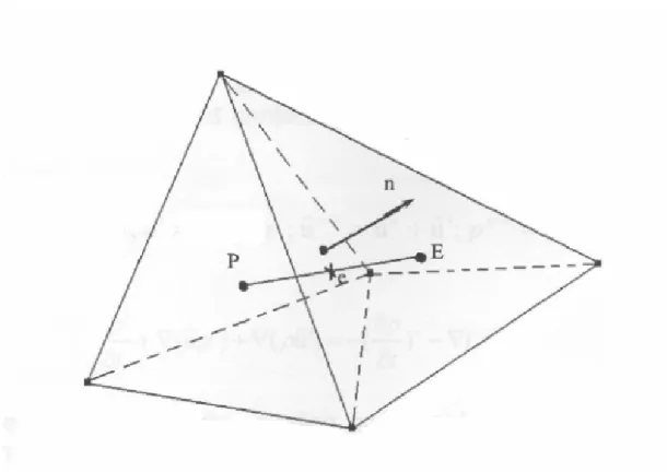
The viscous flux for the face e between control volumes P and E as shown in Fig.2.1 can be approximated as:

(

)

_       − − − ⋅ ∇ + − − ≈ ⋅ ∇ r r r r n r r n E P E e P E P E e r r r r r r r r

φ

(5)

That is based on the consideration that

φ

_E −

φ

_P ≈∇

φ

_e⋅

(

rr_E −rr_P

)

(6) where ∇ is interpolated from the neighbor cells E and P.

φ

The inviscid flux is evaluated through the values at the upwind cell and a linear reconstruction procedure to achieve second order accuracy

(22)

where the subscript u represents the upwind cell and Ψ is a flux limiter used to _e prevent from local extrema introduced by the data reconstruction. The flux limiter proposed by Barth [5] is employed in this work. Defining

(

φ

u

φ

j

)

φ

(

φ

u

φ

j

)

φ

_max =max , , _min =min , , the scalar Ψ associated with the gradient at _e cell u due to edge e is

         < −       − − > −       − − = Ψ 1 0 , 1 min 0 , 1 min 0 0 min 0 0 max

φ

e u e u e u e u e if if (8)

where

φ

_e0 is computed without the limiting condition (i.e. Ψ =1) _e

2.3 Time Integration

A general implicit discretized time-marching scheme for the transport equations can be written as:

ρ

φ

(

ρφ

)

S_φ t A A t n P n m NB m m n P P n + ∆ + =       + ∆ + = +

∑

1 1 1 (9)

where NB means the neighbor cells of cell P. The high order differencing terms and cross diffusion terms are treated using known quantities and retained in the source term and updated explicitly.

(23)

ρ

A

φ

A

φ

SU_φ t m NB m m P P n + ∆ = ∆       + ∆

∑

=1 (10) θ φ φ φ φ       − ∆ + =

∑

= n P n m NB m m A A S SU 1 (11)

where θ is a time-marching control parameter which needs to specify. θ = 1 and θ = 0.5 are for implicit first-order Euler time-marching and second-order time-centered time-marching schemes. The above derivation is good for non-reacting flows. For general applications, a dual-time sub-iteration method is now used in UNIC-UNS for time-accurate time-marching computations.

2.4 Pressure-Velocity-Density Coupling

In an extended SIMPLE [6] family pressure-correction algorithm, the pressure correction equation for all-speed flow is formulated using the perturbed equation of state, momentum and continuity equations. The simplified formulation can be written as: u D p u u u p p p RT n n n n u∇ ′ = + ′ = + ′ − = ′ ′ = ′ +1 +1 ; ; ;r r r r γ ρ ρ (12)

(

)

(

)

( )

n n u t u u t r r r

ρ

∇ −       ∂ ∂ − = ′ ∇ + ′ ∇ + ∂ ′ ∂ (13)

where Du is the pressure-velocity coupling coefficient. Substituting Eq. (12) into Eq. (13), the following all-speed pressure-correction equation is obtained,

(24)

(

)

( )

n n u u t p D t p RT r

ρ

γ

 −∇⋅     ∆ ′ ∆ − = ′ ∇ ⋅ ∇ + ∆ ′ ⋅ 1 (14)

For the cell-centered scheme, the flux integration is conducted along each face and its contribution is sent to the two cells on either side of the interface. Once the integration loop is performed along the face index, the discretization of the governing equations is completed. First, the momentum equation (9) is solved implicitly at the predictor step. Once the solution of pressure-correction equation (14) is obtained, the velocity, pressure and density fields are updated using Eq. (12). The entire corrector step is repeated 2 and 3 times so that the mass conservation is enforced. The scalar equations such as turbulence transport equations, species equations etc. are then solved sequentially. Then, the solution procedure marches to the next time level for transient calculations or global iteration for steady-state calculations. Unlike for incompressible flow, the pressure-correction equation, which contains both convective and diffusive terms is essentially transport-like. All treatments for inviscid and the viscous fluxes described above are applied to the corresponding parts in Eq. (14).

2.5 Linear Matrix Solver

(25)

algebra equations, which are non-symmetric matrix system with arbitrary sparsity patterns. Due to the diagonal dominant for the matrixes of the transport equations, they can converge even through the classical iterative methods. However, the coefficient matrix for the pressure-correction equation may be ill conditioned and the classical iterative methods may break down or converge slowly. Because satisfaction of the continuity equation is of crucial importance to guarantee the overall convergence, most of the computing time in fluid flow calculation is spent on solving the pressure-correction equation by which the continuity-satisfying flow field is enforced. Therefore the preconditioned Bi-CGSTAB [7] and GMRES [8] matrix solvers are used to efficiently solve, respectively, transports equation and pressure-correction equation.

2.6 Parallelization

Compared with a structured grid approach, the unstructured grid algorithm is more memory and CPU intensive because “links” between nodes, faces, cells, needs to be established explicitly, and many efficient solution methods developed for structured grids such as approximate factorization, line relaxation, SIS, etc. cannot be used for unstructured methods.

(26)

expensive even with today’s high-speed computers. As it is becoming more and more difficult to increase the speed and storage of conventional supercomputers, a parallel architecture wherein many processors are put together to work on the same problem seems to be the only alternative. In theory, the power of parallel computing is unlimited. It is reasonable to claim that parallel computing can provide the ultimate throughput for large-scale scientific and engineering applications. It has been demonstrated that performance that rivals or even surpasses supercomputers can be achieved on parallel computers.

(27)

CHAPTER 3 Explanation of Terms

Before the main section of this thesis, here are some important terms to introduce, that is, the Isp, thrust, O/F ratio and regression rate.

3.1 Isp

Specific impulse (usually abbreviated Isp) is a way to describe the efficiency of

rocket and jet engines. It represents the impulse (change in momentum) per unit of

propellant. The higher the specific impulse, the less propellant is needed to gain a

given amount of momentum. Isp is a useful value to compare engines, much like

"miles per gallon" or "liters per kilometer" is used for cars. A propulsion method with

a higher specific impulse is more propellant-efficient.

Propellant is normally measured either in units of mass, or in units of weight at sea

level on the Earth. If mass is used, specific impulse is an impulse per unit mass, which

dimensional analysis shows to be a unit of speed, and so specific impulses are often

measured in meters per second, and are often termed effective exhaust velocity.

However, if propellant weight is used instead, an impulse divided by a force

(weight) turns out to be a unit of time, and so specific impulses are measured in

(28)

a factor of g, the dimensioned constant of gravitational acceleration at the surface of

the Earth.

Specific impulse Isp can be obtained from：

where:

F = gross rocket engine thrust, N = mass flow rate of exhaust gas, kg/s

Ve = exhaust gas velocity at nozzle exit, m/s

Veq = equivalent (or effective) exhaust gas velocity at nozzle exit, m/s Isp = specific impulse, s

go = Gravitational acceleration at sea level on Earth = 9.807 m/s²

where:

Ve = Exhaust velocity at nozzle exit, m/s T = absolute temperature of inlet gas, K

R = Universal gas law constant = 8314.5 J/(kmol·K)

M = the gas molecular mass, kg/kmol (also known as the molecular weight)

k = cp / cv = isentropic expansion factor

cp = specific heat of the gas at constant pressure cv = specific heat of the gas at constant volume Pe = absolute pressure of exhaust gas at nozzle exit, Pa

P = absolute pressure of inlet gas, Pa

3.2 Thrust

(29)

where

is the propellant mass flow rate, which is the rate of decrease of the vehicle's mass.

In this thesis, Dr. Chen used integral method to calculate the momentum change between inlet and outlet section of nozzle and obtain the thrust.

3.3 O/F ratio

O/F ratio means the mass flow rate ratio of oxidizer over fuel.

Standard O/F ratios：oxidizer and fuel can be completely reacted with each other for every case.

Fuel lean：O/F ratio is larger than the standard O/F ratio. Fuel rich：O/F ratio is bigger than the standard O/F ratio.

11N2O+C4H6=>11N2+4CO2+3H2O Standard O/F=11*44/54=8.96

3.4 Regression Rate

Regression rate means the sublimation rate of fuel and its unit is mm/s. From Fig.3.1, it shows specific impulse versus mixture ratio for several oxidizers with

(30)

HTPB.

As for hybrid-rocket, regression rate=1.0 is good enough.

3.5 Different Aft-Nozzle Flows

Essentially then, for rocket nozzles, the ambient pressure acting over the engine largely cancels but effectively acts over the exit plane of the rocket engine in a rearward direction, while the exhaust jet generates forward thrust.

Fig 3.2 shows different aft-nozzle flows. Nozzle flow can be under-expanded, ambient or over-expanded. It depends on the geometry of nozzle. If under or over-expanded then loss of efficiency occurs. Grossly over-expanded nozzles have improved efficiency, but the exhaust jet is unstable.

Under-expended nozzle：In-nozzle pressure is higher than outside pressure. Ambient pressure nozzle：In-nozzle pressure is the same with outside pressure. Over-expended nozzle：In-nozzle pressure is lower than outside pressure.

(31)

3.6 Chemical Reaction

The main chemical reaction is on the first line. And all the reactions would occur in fuel lean or fuel rich situation.

(32)

CHAPTER 4 Results and Discussion

4.1 Overview

In this thesis, I used the hybrid rocket model established by Dr. Chen and

transformed it into the size of our experimental model. First, we established a basic model and analyzed the results. Then we changed some details based on this model like pintle injector area ratio, port size, combustion chamber size, inlet oxidizer mass flow rate and inlet geometry. Finally, we compared the results of the above cases with the basic model and analyzed the results.

Note：All the resultant contours are at the final time-step of simulation.

4.2 Basic Hybrid Rocket Model

Fig. 4.1 shows the basic model and Fig. 4.2 shows the special pintle injector design, they are all designed by Dr. Chen. This pintle injector is used to efficiently direct the inlet flow into the pre-combustion chamber. It can also maintain a low temperature region around it to protect itself. Based on this model, I copied it and transformed it into our test model size. The difference between original and test model is the diameter：Doriginal=132mm and Dtest=72mm.

(33)

4.2.1 Mesh Contour

The contour and size of test model can be seen in Fig. 4.3, this is an axisymmetric model. In Fig. 4.4, it shows four different parts of hybrid rocket.

Part 1：Inlet part of oxidizer with pintle injector

The pintle injector is used to direct the oxidizer into the pre-combustion chamber with an adjusted angle.

Part 2：pre-combustion chamber

It’s used to increase the efficiency of oxidizer decomposition. Part 3：The gray region is the fuel “HTPB” and white region is port. Part 4：post-combustion chamber and nozzle

The purpose of this part is to create more space for the reaction between oxidizer and fuel.

4.2.2 Boundary Conditions

This is a 2D axisymmetry model. 1. Time steps：

Fig 4.5 shows the time line. a. 0~50000：procedure1 b. 50000~70000：procedure2

(34)

c. 0~200：First ignition

d. 3000~3200：Second ignition (Unit：1E-6s)

0~200 and 3000~3200 time-step are the ignition section in procedure1. In simulation, we set a circular region with fixed energy near the front-end of fuel for ignition.

Inlet pressure in procedure1 is set for fixing pressure, but it’s not reasonable in real rocket test. It must be quasi-steady, that is, the interior flow would oscillate. So the pressure is set for fixing total pressure in procedure2. The pressure in procedure2 is obtained from the final state of procedure1.

(35)

2. Material fraction, P and T：

N2O (%) C4H6 (%) N2 (%) O2(%) T(K) P(atm)

Inlet 100 0 0 0 300 20 Outlet 0 0 77.78 22.22 300 20 Fuel 0 100 0 0 820 (fixed) 20 Wall 0 0 77.78 22.22 300 20 Symmetry 0 0 77.78 22.22 300 20

This is the initial boundary condition, fraction of N2 and O2 on the boundaries outlet, wall and symmetry changed as time goes by.

Here the temperature on fuel boundary is fixed equal to 820K because it’s the sublimation temperature of C4H6. We must make sure that C4H6 continually sublimates. Temperature of inlet, outlet and symmetry are not fixed.

3. Oxidizer mass flow rate： mfuel = regression rate*ρHTPB*A

(36)

moxidizer = mfuel*O/F=0.0575*3.9=0.1979 kg/s uin = mN2O/(ρN2O*Ain) ρN2O=35.74 (20atm) Ain= 103.82*10 6 − (m3) uin = 0.1979/(35.74*103.82)=53.33 m/s

O/F ratio is obtained from Dr. Chen’s model. ρHTPB is obtained from solid C4H6.

Regression rate=1.5*10−3(s) is an ideal number.

4.2.3 Results

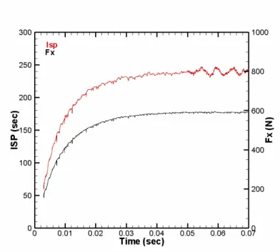
Fig 4.6 shows Isp and Fx versus time of the basic model. Red line represents Isp and

black line represents Fx. Before time=0.04, it’s under developed. And after time=0.05,

the procedure2 is set for fixing total pressure. We can see that Isp oscillate and is maintained under quasi-steady condition.

Fig 4.7~4.9 show the temperature, oxygen and pressure contours of the basic model. These results are at the final time-step state and in fact the waves inside them would change with time. Temperature changed from 300K to 3300K, oxidizer mole fraction changed from 0 to 0.34, and the pressure changed from 0 to 18 atm. Inside-pressure maintains at about 18atm.

(37)

From Fig 4.7, we can see that temperature is under unstable condition near the inlet and becomes stable in the port. The temperature near pintle injector is below 500K, it’s quite low, thus pintle injector would not hurt by the high temperature and can be reused for many times.

Fig. 4.8 shows that in the pre-combustion chamber the oxidizer mole fraction is near zero. Oxidizer injects into this region and be decomposed immediately then reacts with the fuel. As a result, oxidizer is almost reacted with the fuel. As for the post-combustion chamber, oxidizer can hardly flow into this region, if oxidizer flows in, it must be reacted with oxidizer immediately. So the oxidizer mole fraction is near zero in this region. And the oxygen is not consumed efficiently near the axis.

From Fig. 4.9, the pressure inside the combustion chamber is uniform and maintains at about 18 atm.

Fig. 4.10 is the streamline contour at the final step, it changes as time goes by. It shows that, in the pre-combustion chamber, the oxidizer separates into two flows. And it is efficiently directed into the pre-combustion chamber. As a result, the oxidizer can almost be decomposed and then reacts with fuel, thus increases the regression rate.

(38)

4.3 Results of Different Test Conditions in Combustion Chamber

Based on Basic Model and Comparison with Basic Model

This paper changes some details in the combustion chamber of hybrid rocket, that is, the area ratio of pintle injector, port size, pre-chamber size, inlet oxidizer mass flow rate and the inlet geometry, then compares the results with the basic model and analyzes the results.

4.3.1 Different Inlet Area Ratios of Pintle injector

4.3.1.1 Mesh Contours

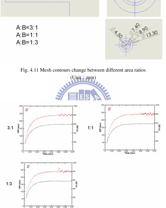
Mesh contours change can be seen from Fig 4.11. The area ratio of basic model is about 3:1 and we moved the side baffle-plate to make inside flow region larger. The second and third area ratios are A:B=1:1 and A:B=1:3.

4.3.1.2 Boundary Conditions

The boundary conditions here are the same with the basic model. The inlet mass flow rate is also fixed equal to 0.1979 kg/s.

(39)

4.3.1.3 Results and Comparison

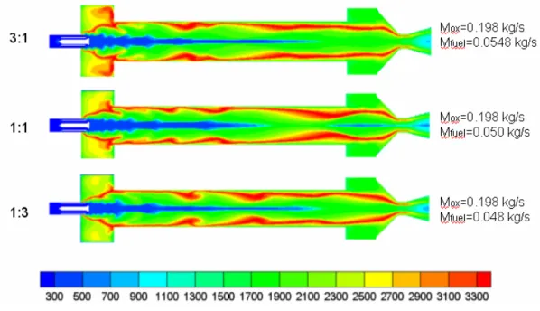
Fig. 4.12 shows that all the results of different area ratios maintain at quasi-steady condition at the final time-step.

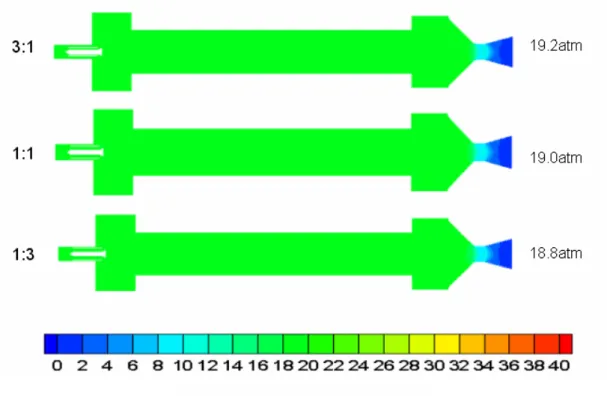
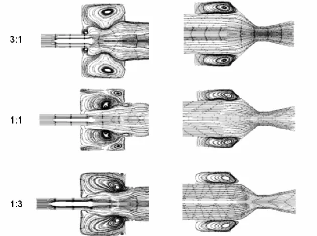
Fig 4.13~4.15 show the temperature, oxygen and pressure contours comparison between different area ratios. Fig4.16 and 4.17 show the streamline. Pressures are almost the same.

From Fig 4.17 we can observe that, with the increase of the inside flow area, the aft-pintle injector flow angle become smaller and there’s more fraction of oxidizer is directed into the port. Under this situation, oxidizer can not be decomposed

efficiently, thus the decomposed fuel becomes fewer and the regression rate decreases. From Fig. 4.13, this phenomenon also decreases the reaction efficiency between oxidizer and fuel in the pre-combustion chamber, thus decreases the temperature in it.

From table 4.2 we can observe this phenomenon. Regression rate and Fx of A:B=1:1 and A:B=1:3 become lower. On the other hand, O/F ratio becomes higher because of lower fuel sublimation rate.

(40)

4.3.2 Different Pre-Combustion Chamber Sizes

4.3.2.1 Mesh Contours

Mesh contours change can be seen from Fig 4.18. The chamber size of the basic model is 36mm. We increased the chamber size to 60mm and 90mm. Then we analyzed the results.

4.3.2.2 Boundary Conditions

The boundary conditions here are the same with the basic model. The inlet mass flow rate is also set for 0.1979 kg/s.

4.3.2.3 Results and Comparison

Fig4.19 shows that all the results of different chamber sizes maintain at quasi-steady condition at the final time-step.

Fig. 4.20~4.22 show the temperature, oxygen and pressure contours between different chamber sizes. From Fig. 4.20 and Fig. 4.21, we can see that the temperature increases when the chamber size becomes longer. It’s because oxidizer is well

decomposed and reacts with fuel, thus the temperature in pre-combustion chamber increases. And the right part in Fig. 4.20 shows that the fuel sublimation rate becomes

(41)

higher.

From Fig. 4.23 and Fig. 4.24, the streamline contours show the oxidizer flowing into port becomes smoother if the sizes of pre-combustion chamber are increased. Averaged regression rate and Fx in table 4.3 both indicate that if we increased the chamber sizes, they increase, too. But the increase from 60mm to 90mm is not that obvious as increase from 36mm to 60mm. So the chamber size=60mm is useful enough.

4.3.3 Different Fuel Port Sizes

4.3.3.1 Mesh Contours

Mesh contours change can be seen from Fig 4.25. The port size of the basic model is 40mm. We had tested two more different port sizes, that is, 50mm and 60mm. These tests can also be regarded as different situations changing with time in the hybrid rocket tests. But the real port contours are not that smooth compared with them.

4.3.3.2 Boundary Conditions

The boundary conditions here are the same with the basic model. The inlet mass flow rate is set for 0.1979 kg/s.

(42)

4.3.3.3 Results and Comparison

Fig4.26 shows that all the results of different port sizes maintain at quasi-steady condition at the final time-step.

Fig. 4.27~4.29 show the temperature, oxygen and pressure contours of different port sizes. Fig. 4.30 and 4.31 show the streamline contours. Temperature contour indicates that when the port size becomes larger, because the oxidize inlet angle is fixed, oxidizer can not be directed into pre-combustion chamber efficiently. Thus high temperature region in pre-combustion chamber become smaller. This phenomenon can be observed from Fig. 4.30 and Fig. 4.31. In Fig. 4.27, the right part shows that the fuel mass flow rates are almost the same. And because contact areas become larger, oxygen consumption efficiency in larger port sizes becomes higher.

From Fig.4.29, the three pressures increases with the increase of port diameter. But these three pressures are almost the same.

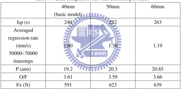
Finally, from table 4.4, it can be easily observed that with the increase of port size, the averaged regression rate becomes lower. With almost the same fuel sublimation, the port size becomes larger and surface area increases too. Under this situation, the regression rate decreases. On the contrary, Fx increases because of efficient reaction between oxidizer and fuel.

(43)

4.3.4 Different Inlet Oxidizer Mass Flow Rates

4.3.4.1 Boundary Conditions

Here the inlet oxidizer mass flow rates are set for different numbers. The basic model is set for 0.198 kg/s. Then we changed it by 0.1 kg/s, 0.3 kg/s and 0.4 kg/s. Then we compared the results.

4.3.4.2 Results and Comparison

Fig. 4.32 shows that all the results of different inlet oxidizer mass flow rates maintain at quasi-steady condition at the final time-step..

Fig. 4.33~4.35 show the temperature, oxidizer and pressure contours. From Fig. 4.33, it can be seen that with the increase of inlet oxidizer mass flow rate, more oxidizer flows into pre-combustion chamber, decomposes and reacts with fuel, thus increases the temperature in pre-combustion chamber. This phenomenon can also be observed from Fig. 4.34, there’s more oxygen in the pre-combustion chamber if we increased the inlet oxidizer mass flow rate. In Fig. 4.35, because that more oxidizer flows in, there’s more fuel sublimates and reaction efficiency becomes higher between oxidizer and fuel, there’s more gas inside the combustion chamber. And the pressure increases.

(44)

oxidizer mass flow rates. It can be observed that the flows are almost the same. Finally, from table 4.5, regression rates, O/F ratio and Fx both become higher when the oxidizer mass flow rate increases. From these results, increasing the inlet oxidizer mass flow rate seems to be a good way to increase Fx. But the pressure maybe higher than pressure in the oxidizer chamber and would cause danger.

4.3.5 Redesigned Geometries of Injector

4.3.5.1 Mesh Contours

Mesh contours can be seen from Fig. 4.38 and 4.39. Besides the basic aslope pintle injector model, we established an axial model without pintle injector and a radial model that changed the pintle injector geometry into vertical injector that directs the oxidizer into the pre-combustion chamber.

4.3.5.2 Boundary Conditions

The boundary conditions here are the same with the basic model. The inlet mass flow rate is also set for 0.1979 kg/s.

(45)

4.3.5.3 Results and Comparison

Fig4.40 shows that all the results of different injector geometries maintain at quasi-steady condition at the final time-step.

Fig. 4.41~4.43 show the temperature, oxygen and pressure contours. From

temperature contour, we can see the oxidizer in the axial model flows directly into the port and the fuel sublimation rate becomes lower than the basic model. On the other hand, the radial model shows better oxidizer decomposition efficiency in the

pre-combustion chamber and the fuel sublimation rate becomes higher than the basic model. But the temperature around this pintle injector is about 1700K~1900K. It’s too high and might have bad influence on the pintle injector.

From Fig. 4.42, oxygen fraction near the outlet of axial model is still high and there’s much oxygen is not consumed. Nevertheless, the radial model shows better oxygen consumed efficiency than the basic model.

Fiig 4.43 shows that the axial injector pressure is lower than the basic pintle injector. Nevertheless, radial injector pressure is higher than the basic model. This is because of different reaction efficiency between oxidizer and fuel in the combustion chamber. Radial injector has better oxidizer decomposition and reaction efficiency, thus more gas can be produced and increases the pressure. Axial injector is on the contrary with radial injector.

(46)

Fig 4.44 and 4.45 show the streamline contours of these three geometries. In the axial model, most of the oxidizer flows into the port. As for the radial model, oxidizer flows vertically into the pre-combustion chamber. And there are some circulations near the pintle injector that cause high temperature.

Table 4.6 shows that the regression rate, pressure and Fx of the axial model is lower than the basic aslope model. And these data of the radial model is higher than the basic aslope model.

(47)

CHAPTER 5 Concluding Remarks and Recommendations for

Future Work

5.1 Results and Discussion

This thesis lists five groups of different tests.

1. In the first test, we changed the area ratio of the pintle injector. From the results, the area ratio A:B=1:3 has better flow direction. The results indicate that its oxidizer inflow angle is more suitable for this model. In conclusion, moving the side baffle-plate is a good way to test a suitable angle which can direct the oxidizer into the pre-combustion chamber smoothly.

2. In the second test, we changed the chamber size. As a result, chamber size is equal to 60mm is the best one when considering its performance and size. 3. In the third test, we changed the port size. This can also be regarded as the

different combustion situations in different times. The results show that with the increase of the port size, thrust increases because of larger contact space

between oxidizer and fuel. Nevertheless, in real test, the oxidizer mass flow rate decreases as time goes by because of pressure drop in the oxidizer chamber, thus influences the results. So the real thrust will not be that large as our simulation. Nevertheless, simulation is still a good way to get the combustion trends.

(48)

4. In the fourth test, we changed the oxidizer mass flow rate. With the increase of it, thrust, pressure and regression rate all increase. But it must be careful that if the oxidizer mass flow is too high, pressure in the combustion chamber will be higher than oxidizer chamber pressure and it would cause danger.

5. In the fifth test, we changed the inlet geometry. As our prediction, axial model has lower regression rate and thrust. And there is more oxygen not used. As for the radial model, it has better regression rate and thrust. Without its high

temperature near the pintle injector region, this pintle injector is the best among them.

5.2 Recommendations for Future Work

So far we have only simulated the 2D experimental model. The full size 2D model simulation is also needed in the future. The 3D simulation must depend on the design of experimental group.

All the results are obtained from inlet boundary condition with pure gas state. But in reality, it must combines gas and liquid state. And the liquid state oxidizer will absorb heat in order to transform into gas state. Thus temperature in combustion chamber will decrease. Constructing a real fluid model is a good way to solve this problem. And simulation must include oxidizer camber to obtain more accurate data.

(49)

When compared with the experimental group, it shows better results in the

numerical simulation. Because the oxidizer is not pure gas state in the real condition, the highest temperature will not be 3300K, it must drops. The fuel geometry is one of the concerned factors. Fuel port geometry in the numerical simulation is quite smooth. In the real situation, fuel port geometry changes all the time. It will not be that smooth as numerical simulation geometries. And finally, inflow oxidizer mass flow rate changes with the oxidizer chamber pressure, thus it must decrease as time goes by. So the inflow oxidizer mass flow rate must decreases with increase of port sizes. It’s better to discuss with the experimental group and use their data to run the numerical simulation.

(50)

REFERENCES

[1.1] Computational Fluid Dynamics Modeling Hybrid Rocket Flowfields American Institute of Aeronautics and Astronautics

Venkateswaran Sankaran*

Purdue University, West Lafayette, Indiana 47907

[1.2] Fundamentals of Hybrid Rocket Combustion and Propulsion Edited by：Martin J. Chiaverini

Orbital Technologies Corporation (ORBITEC), Madison, Wisconsin

Kenneth K. Kuo

Pennsylvania State University, University Park, Pennsylvania Progress in Astronautics and Aeronautics

Frank K. Lu, Editor-in-Chief

University of Texas at Arlington, Arlington, Texas

[1.3] Influence of a Conical Axial Injector on Hybrid Rocket Performance Carmine Carmicino* and Annamaria Russo Sorge

Journal of Propulsion and Power

University of Naples “Federico II,” 80125 Napoli, Italy Vol. 22, No. 5, September-October 984-995 2006

(51)

[1.4] Performance Comparison Between Two Different Injector Configurations in a Hybrid Rocket

Aerospace Science and Technology 11 (2007) 61-67 Carmine Carmicino* and Annamaria Russo Sorge University of Naples “Federico II,” 80125 Napoli, Italy

[1.5] Review of Solid-Fuel Regression Rate Behavior in Classical and Nonclassical Hybrid Rocket Motors

American Institute of Aeronautics and Astronautics Martin Chiaverini*

Orbital Technologies Corporation, Madison, Wisconsin 53717 [1.6] Role of Injection in Hybrid Rockets Regression Rate Behavior

Carmine Carmicino* and Annamaria Russo Sorge Journal of Propulsion and Power

University of Naples “Federico II,” 80125 Napoli, Italy Vol. 21, No. 4, July-August 606-612 2005

(52)

Appendix

Tables

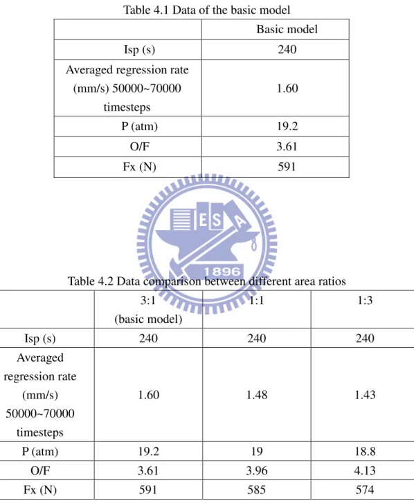
Table 4.1 Data of the basic model Basic model

Isp (s) 240

Averaged regression rate (mm/s) 50000~70000 timesteps 1.60 P (atm) 19.2 O/F 3.61 Fx (N) 591

Table 4.2 Data comparison between different area ratios 3:1 (basic model) 1:1 1:3 Isp (s) 240 240 240 Averaged regression rate (mm/s) 50000~70000 timesteps 1.60 1.48 1.43 P (atm) 19.2 19 18.8 O/F 3.61 3.96 4.13 Fx (N) 591 585 574

(53)

Table 4.3 Data comparison between different chamber sizes 36mm (basic model) 60mm 90mm Isp (s) 240 240 241 Averaged regression rate (mm/s) 50000~70000 timesteps 1.60 1.69 1.71 P (atm) 19.2 19.4 19.6 O/F 3.61 3.46 3.42 Fx (N) 591 598 601

Table 4.4 Data comparison between different port sizes 40mm (basic model) 50mm 60mm Isp (s) 240 252 263 Averaged regression rate (mm/s) 50000~70000 timesteps 1.60 1.38 1.19 P (atm) 19.2 20.3 20.85 O/F 3.61 3.59 3.66 Fx (N) 591 623 639

Table 4.5 Data comparison between different inlet oxidizer mass flow rates 0.1 0.198 (basic model) 0.3 0.4 Isp (s) 234 240 241 243 Averaged regression rate (mm/s) 50000~70000 timesteps 1.07 1.60 2.11 2.56 P (atm) 10.3 19.2 30.0 38.0 O/F 2.82 3.61 4.26 4.64 Fx (N) 316 591 889 1170

(54)

Table 4.6 Data comparison between different injector geometries Aslope (basic model) Axial Radial Isp (s) 240 245 251 Averaged regression rate (mm/s) 50000~70000 timesteps 1.60 1.11 1.94 P (atm) 19.2 18.1 21.1 O/F 3.61 5.21 2.91 Fx (N) 591 553 649

(55)

Figures

(56)

Fig. 2.1 Vacuum Isp vs O/F Mass Mixture Ratio with HTPB

(57)

Fig. 4.1 Basic hybrid rocket model made by Dr. Chen (Unit：mm)

Fig. 4.2 Pintle injector of Dr. Chen’s basic model (Unit：mm)

(58)

Fig. 4.3 Redesigned test model based on Dr. Chen’s model (Unit：mm)

Fig. 4.4 Different parts in hybrid-rocket combustion chamber

(59)

Fig. 4.6 Isp and Fx versus time of the basic model

Fig. 4.7 Temperature contour of the basic model (Unit：K)

Fig. 4.8 Oxygen contour of the basic model (Unit：mole fraction)

(60)

Fig. 4.9 Pressure contour of the basic model (Unit：atm)

(61)

Fig. 4.11 Mesh contours change between different area ratios (Unit：mm)

(62)

Fig. 4.13 Temperature contours comparison between different area ratios (Unit：K)

Fig. 4.14 Oxygen contours comparison between different area ratios (Unit：mole fraction)

(63)

Fig. 4.15 Pressure contours comparison between different area ratios (Unit：atm)

(64)

(65)

Fig. 4.18 Mesh contours between different chamber sizes (Unit：mm)

(66)

Fig. 4.20 Temperature contours comparison between different chamber sizes (Unit：K)

Fig. 4.21 Oxygen contours comparison between different chamber sizes (Unit：mole fraction)

(67)

Fig. 4.22 Pressure contours comparison between different chamber sizes (Unit：atm)

(68)

(69)

Fig. 4.25 Mesh contours between different port sizes (Unit：mm)

(70)

Fig. 4.27 Temperature contours comparison between different port sizes (Unit：K)

Fig. 4.28 Oxygen contours comparison between different port sizes (Unit：mole fraction)

(71)

Fig. 4.29 Pressure contours comparison between different port sizes (Unit：atm)

(72)

(73)

Fig. 4.32 Isp and Fx comparison between different inlet oxidizer mass flow rates

Fig. 4.33 Temperature contours comparison between different inlet oxidizer mass flow rates (Unit：K)

(74)

Fig. 4.34 Oxygen contours comparison between different inlet oxidizer mass flow rates (Unit：mole fraction)

Fig. 4.35 Pressure contours comparison between different inlet oxidizer mass flow rates (Unit：atm)

(75)

Fig. 4.36 Streamline contours comparison between different inlet oxidizer mass flow rates

(76)

Fig. 4.37 Detailed streamline contours comparison between different inlet oxidizer mass flow rates

(77)

Fig. 4.38 Basic pintle injector model geometres (Unit：mm)

Fig. 4.39 Mesh contour of axial and radial injector model geometries (Unit：mm)

(78)

Fig. 4.40 Isp and Fx comparison between different injector geometries

Fig. 4.41 Temperature contours comparison between different injector geometries (Unit：K)

(79)

Fig. 4.42 Oxygen contours comparison between different injector geometries (Unit：mole fraction)

Fig. 4.43 Pressure contours comparison between different injector geometries (Unit：atm)

(80)

Fig. 4.44 Streamline contours comparison between different injector geometries

Fig. 4.45 Detailed streamline contours comparison between different injector geometries

(81)

依據混合式火箭實驗模型以數值模擬分析其 燃燒引擎的燃燒推進過程的研究

國立交通大學

機械工程學系

碩士論文

CFD Simulation on Model of the Experimental

Hybrid-Rocket Motor

依據混合式火箭實驗模型以數值模擬分析其

燃燒引擎的燃燒推進過程的研究

指導教授：吳宗信博士

研究生：林俊傑

中華民國九十八年七月

依據混合式火箭實驗模型以數值模擬分析其

依據混合式火箭實驗模型以數值模擬分析其

依據混合式火箭實驗模型以數值模擬分析其

依據混合式火箭實驗模型以數值模擬分析其

燃燒引擎的燃燒推進過程的研究

燃燒引擎的燃燒推進過程的研究

燃燒引擎的燃燒推進過程的研究

燃燒引擎的燃燒推進過程的研究

CFD Simulation on Model of the Experimental

Hybrid-Rocket Motor

研究生

研究生

研究生

研究生：

：

：

：林俊傑

林俊傑

林俊傑

林俊傑

Student: Jyun-Jie Lin

指導教授

指導教授

指導教授

指導教授：

：

：

：吳宗信博士

吳宗信博士

吳宗信博士

吳宗信博士

Advisor: Dr. Jong-Shinn Wu

國立交通大學

機械工程學系

碩 士 論 文

A Thesis

Submitted to Department of Mechanical Engineering

National Chiao Tung University

in Partial Fulfillment of the Requirements

for the Degree of

Master of Science

In

Mechanical Engineering

July 2009

Hsinchu, Taiwan

2009 年 七月

ABSTRACT

誌謝

誌謝

誌謝

誌謝

首先感謝我的家人，在我的求學道路上一路支持下去，現在才得以完

成碩士班的學位。接著在碩士班的兩年中，特別感謝吳宗信老師的教

導，在每一次的報告中，總是很有耐心的聽著報告內容，並且在之後

提出不足和需要改進的部分，遇到我沒辦法立刻理解的情況，

吳老師會不厭其煩重複地教導，直到了解為止，我很榮幸能在此實驗

室待這兩年，吳老師對於當前的科技發展狀況一直都有很特別獨到的

見解，讓我受益良多。

另外，也要特別感謝林昆模學長，在接下公司的案子時，不斷的教

導我做投影片的技巧、報告方式以及如何處理廠商要求的進對應退技

巧；感謝 Aziz 在我心煩時會和我聊天，交流台灣和法國的文化，並

且抒發 Aziz 有趣的思想。

感謝 APPL 實驗室提供足夠的資源，讓我能在研究所兩年的時間裡

對於研究的資源充足。

感謝鄭凱文、李允民、洪捷粲、邱老大、江明鴻、胡孟樺、林雅茹、

林昆模、盧勁全、林宗漢、洪維呈等諸位學長姐，感謝他們不厭其煩

的為我在研究以及其他方面解惑。感謝王穎志、古必任以及林逸民諸

位同學，感謝有你們和我一起在研究上互相勉勵和進步。感謝周子

豪、吳尚穎、呂其璋、黃皓遠諸位學弟、前助理于恩以及現任助理王

依據混合式火箭實驗模型以數值模擬分析其燃燒引擎的燃燒推進過程的研究

碩士論文

2009 年七月

₍

₎