使用不同斜率的限制在半離散中央上風法對雙曲保守律的數值研究與比較

國立交通大學

應用數學系

碩 士 論 文

使用不同斜率的限制在半離散中央上風法對雙曲保

守律的數值研究與比較

Numerical study and comparison of semidiscrete

central-upwind schemes for hyperbolic conservation laws

with different slope limiters

研 究 生：張佑民

指導教授：薛名成 教授

使用不同斜率的限制在半離散中央上風法對雙曲保守律的

數值研究與比較

Numerical study and comparison of semidiscrete

central-upwind schemes for hyperbolic conservation laws with

different slope limiters

研 究 生：張佑民

指導教授：薛名成

教授

Student: Yu-Ming Chang

Advisor: Ming-Cheng Shiue

國 立 交 通 大 學

應 用 數 學 系

碩 士 論 文

A Thesis

Submitted to Department of Applied Mathematics

College of Science

National Chiao Tung University

in Partial Fulfillment of the Requirements

for the Degree of

Master

in

Applied Mathematics

July 2013

Hsinchu, Taiwan, Republic of China

使用不同斜率的限制在半離散中央上風法對雙曲保

守律的數值研究與比較

學生：張佑民

指導教授：薛名成

教授

國立交通大學應用數學系（研究所）碩士班

摘

要

本論文，我們研究對雙曲保守律的數值近似方法。我們使用有反擴散項的半離散中央上 風法，在重構和投影的步驟裡使用不同的斜率限制，而這些我們所選取的斜率限制它滿 足單調的特性。此外我們呈現使用不同斜率限制的數值結果並且進行比較。在第一章 節，我們簡單介紹雙曲保守律和一些計算這類系統的數值方法。在第二章節，我們在新 半離散中央上風法裡的重構和投影步驟中使用不同的斜率限制。在第三章節，我們探討 選取的數值通量滿足單調特性。在第四章節，我們呈現數值結果並且觀察它們的特性。 關鍵詞：雙曲保守律、半離散中央上風法、數值耗散。

Numerical study and comparison of semidiscrete

central-upwind schemes for hyperbolic conservation

laws with different slope limiters

Student: Yu-Ming Chang

Advisors: Ming-Cheng Shiue

Department (Institute) of Applied Mathematics

National Chiao Tung University

Abstract

In this thesis, we study numerical approximation for hyperbolic conservation laws arising from physical models. In particular, we introduce modified and new semidiscrete central-upwind schemes with different slope limiters, which are believed to monotone scheme, to reduce numerical dissipation. Furthermore, we compare and present numerical results with different slope limiters.

In Chapter 1, we briefly introduced hyperbolic conservation laws. We also recalled numerical methods for this type of equations in the literature. In particular, we consider a Godunov-type finite volume scheme.

In Chapter 2, we followed the ideas on less numerical dissipative numerical schemes for hyperbolic conservation laws schemes as in [6]. Our goal is to reduce numerical dissipation and to obtain more accurate solutions. Then we use different limiters at reconstruction and evolution step in these new semidiscrete up-wind schemes.

In Chapter 3, we discussed that the numerical fluxes we choose satisfy the monotonic property.

In Chapter 4, we presented some numerical resolutions and observed performance of the new second-order semidiscrete central-upwind schemes.

Keywords: Hyperbolic systems of conservation laws, semi-discrete central-upwind schemes,

誌

謝

完成這本論文，首先我要感謝我的指導教授 薛名成老師，感謝老師指導和指正論 文上的缺失和疏漏，在過去兩年間的教誨，老師不僅僅教導我解決問題的方法，還有面 對問題跟困難的態度。在碩士生涯中，希望我們不只是在念碩士而已，並要求我們對於 日後有所規劃，對人生有所想法。積極面對問題，克服困難。感謝老師的教誨。同時也 要感謝吳金典教授和卓建宏教授願意擔任我的口試委員。 此 外 我 要 感 謝 研 究 室 的 所 有 成 員 育 磐、 秉 陽、 卓 翰。 除 了 這 兩 年 的 陪 伴，在課業和程式上都樂於幫助我解決問題且也提供了許多寶貴的意見。同時感謝宇鎮 在研究上給我一些建議，分擔我的煩惱。這一路上幸好有你們的相伴，才能讓我走的如 此順利。 最後要感謝在我背後一直支持我的家人，感謝你們一直以來的關心與照顧，雖然 家境不是很好，但是爸爸和媽媽還是很努力的提供我跟別人相同的環境與資源，讓我能 夠無後顧之憂的不斷向前，這份榮耀我希望與你們一同分享。 張佑民 謹誌于交通大學 2013 年 7 月

Contents

Abstract (in Chinese) i Abstract (in English) ii

List of Figures v

1 Introduction 1

2 Semidiscrete central-upwind schemes 3 3 Monotone numerical schemes 14 4 Numerical examples and concluding remarks 22

List of Figures

2.1 Slope limiters . . . 6 2.2 Central-upwind differencing . . . 7

4.1 Example 1 computed by the NEW and OLD second-order schemes with same spatial grid . . . 26 4.2 Example 1 computed by the NEW second-order schemes with five kinds of

limiters . . . 27 4.3 Example 2 computed by the NEW second-order schemes with five kinds of

limiters and zoom at [0.67:0.88] . . . 27 4.4 Example 2 uniform grid with ∆x=1/2400 . . . 27 4.5 Example 3 computed by the NEW second-order schemes with five kinds of

limiters . . . 28 4.6 Exact solution of the shock tube problem at time t=0.2 . . . 28 4.7 Example 4 computed by the OLD and NEW second-order schemes at time

t=0.2 . . . 28 4.8 Same as Figure 4.7 —zoom at [0.45 0.88] . . . 29 4.9 Exact solution of inviscid Burgers’ equation at time t=1 . . . 29 4.10 Example 5 computed by the OLD and NEW second-order schemes at time

t=1 . . . 29 4.11 Same as Figure 4.10 —zoom at [0.85 1.5] . . . 30

Chapter 1

Introduction

We consider the systems of hyperbolic conservation laws with flux vector f(u): ∂

∂tu(x, t) + ∂

∂xf(u(x, t)) = 0. (1.1) The system arises from physical principles such as conservation of mass, momentum,or energy and we refer the reader to see [10, 13] for more detailed information. Such a system aries in many applications such as traffic flow.

As for numerical methods for hyperbolic conservation law (1.1), we often use finite difference [8], finite element [17, 4], and finite volume methods [10, 1, 9]. The finite difference method is the differential operator replaced by finite difference and to use computing grids to construct difference, and approximate derivatives. The finite volume method is to use subdivision of spatial computing domain and computing integral of these control volumes to approximate the flux through the endpoints of the intervals in space dimension one.

The finite volume type that we consider is a Godunov-type scheme. The scheme is to use cell average at time level tn_{, construct piecewise polynomial, evolve at time level t}n+1_,

and finally project onto space of piecewise interpolant (see in [7, 12]).

In this thesis, we use new semidiscrete central-upwind schemes with anti-diffusion terms for hyperbolic conservation laws. We focus on modifying slope limiters that satisfy Total Variation Diminishing Diminishing (TVD) [15] at reconstruction step, choosing the

same slope limiters at projection step and comparing performance of these numerical results with the new semidiscrete central-upwind schemes.

The rest point of this thesis is organized as follows: In Chapter 2, we recall origi-nal semi-discrete central-upwind schemes and introduce new semi-discrete central-upwind schemes with modified limiters. In Chapter 3, monotonicity of numerical schemes derived in Chapter 2 is studied. Finally, we present numerical results and compare numerical solutions with different slope limiters. Furthermore, some concluding remarks are also given in Chapter 4.

Chapter 2

Semidiscrete central-upwind schemes

In this Chapter, we recall the original semidiscrete central-upwind schemes and intro-duce new numerical schemes to reintro-duce the numerical dissipation in the original scheme (see [7]). The motivation comes from the choices of the slope limiters which are introduced to avoid oscillatory.

In this Chapter, we consider the following one dimensional hyperbolic conservation laws:

ut+ f(u)x = 0, (2.1)

where u = u(x, t) : _{R × R}+ _{−→ R}n _{is the unknown, the flux f(u) is a function from R}

to Rn _{and n is a positive integer. Equation (2.1) is hyperbolic if the Jacobian matrix}

(∂fi

∂uj), i, j=1,...n satisfies the property that the matrix has only real eigenvalues and is

diagonalizable.

For the discretization, we consider the uniform grids xj = j∆x, xj±1₂ = (j ±

1 2)∆x

and tn = n∆t where ∆x and ∆t are the mesh size in space and time respectively; j is an

integer and n is positive integer. We denote the cell average un j by 1 ∆x ∫ x_{j+ 1} 2 x_{j− 1} 2 u(x, tn)dx≈ unj, j = 0,±1, ±2, ..., and Ij = (xj−1₂, xj+1₂).

Integrating (2.1) over the space time domain Ij × (tn, tn+1), the resulting equation gives 1 ∆x ∫ tn+1 tn ∫ x_{j+ 1} 2 x_{j− 1} 2 ut(x, t)dxdt = 1 ∆x ( ∫ x_{j+ 1} 2 x_{j− 1} 2 u(x, tn+1)dx− ∫ x_{j+ 1} 2 x_{j− 1} 2 u(x, tn)dx ) = un+1_j − un_j, (2.2) and 1 ∆x ∫ tn+1 tn ∫ x_{j+ 1} 2 x_{j− 1} 2 fx(u(x, t))dxdt = 1 ∆x [ ∫ tn+1 tn ( f(u(x_j+1 2, t))− f(u(xj− 1 2, t)) ) dt ] . (2.3) We can infer from (2.2) and (2.3) that

un+1 j = u n j − 1 ∆x [ ∫ tn+1 tn ( f(u(x_j+1 2, t))− f(u(xj− 1 2, t)) ) dt ] . (2.4)

The construction of central-upwind schemes for one time step consists of three con-secutive steps : reconstruction, evolution and projection back onto the original grid.

The first step is to reconstruct the second-order piecewise linear interpolant such that its averages are equal to the data {un

j}. The second step is to evolve the approximate

solution represented by a global piecewise linear interpolant eu(x, tn), to the next time

level using the integral form of the conservation law (2.4). Finally, we use the piecewise linear interpolant reconstruction from the evolved intermediate cell average, and project back onto the original grids. Now we start to discuss these steps for the detailed procedure as follows:

Reconstruction:

First,we reconstruct the second-order piecewise linear interpolant eu(x, tn) from the

cell averages {un

j}. That is, we find a suitable polynomial pnj(x) such that its cell average

on Ij is equal to unj for j.

More specifically, the slope sn

j is considered as the form of

sn_j = ψ(Rj)(uj− uj−1), (2.6)

where Rn

j is the ratio of forward differences to backward ones in the solution defined as

R_jn= uj+1− uj

uj− uj−1

,

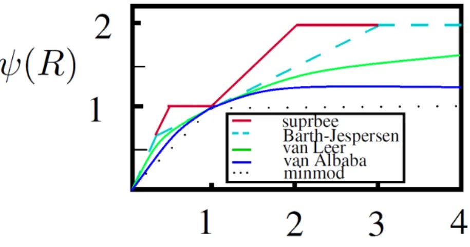
and the limiter ψ is introduced to satisfy the property of Total Variation Diminishing (TVD) and avoid numerical oscillatory. In this thesis, we study five kinds of limiters (superbee, Barth-Jespersen, van Leer, van Albada, and mimod) which have been analyzed in [15, 11]. Now, let us denote the following limiters by

(superbee) ψsb(R) = min[max{1, R}, 2, 2R], (Barth-Jespersen) ψBJ(R) = 1 2(R + 1)min[min(1, 4R R + 1), min(1, 4 R + 1)], (van Leer) ψV L(R) = 2R R + 1, (van Albada) ψV A(R) = R2+ R R2 _{+ 1},

(min) ψmin(R) = min{1, R}.

(2.7)

Notice that for these limiters, a negative value of R indicates an extremum in the solution, and set ψ(R_{≤ 0) = 0. (see Figure 2.1)}

Evolution:

The discontinuities of piecewise polynomial (2.5) may appear at the interface point {x_j+1

2} propagating with right- and left-sides local speeds, which can be computed by

a+_j+1 2 := max ω∈C(u− j+ 1₂,u + j+ 1₂) {λN(A(ω), 0)}, and a−_j+1 2 := min ω∈C(u− j+ 1,u + j+ 1) {λ1(A(ω), 0)}.

Figure 2.1: Slope limiters

Here, λ1 < λ2 < ... < λN are the N eigenvalues of the Jacobian A := _∂u∂f, and

C(u−_j+1 2

, u+_j+1 2

) is the curve in the phase space that connects the left, u−_j+1 2 = lim x→x− j+ 1₂ eu(x, tn ), and the right u+

j+1₂ =_x→xlim+

j+ 1₂

eu(x, tn_{). The local speeds can be estimated by}

a+ j+1₂ := max{λN( ∂f ∂u(u + j+1₂)), λN( ∂f ∂u(u − j+1₂)), 0}, (2.8) and a− j+1₂ := min{λ1( ∂f ∂u(u + j+1₂)), λ1( ∂f ∂u(u − j+1₂)), 0)}. (2.9)

Next, we consider the non-equal rectangular domains

[xn_j−1 2,r , xn_j+1 2,l ]× [tn, tn+1], [xn_j+1 2,l , xn_j+1 2,r ]× [tn, tn+1] where xn j+1₂,l := xj+12 + ∆ta − j+1₂ and x n j+1₂,r := xj+12 + ∆ta + j+1₂(see Figure 2.2).

Integration of (2.1) over these domains, the nonsmooth cell averages are computed by

wn j+1₂ = 1 xn j+1₂,r− x n j+1₂,l [ ∫ x j+ 1₂ xn j+ 1₂,l pn_j(x)dx + ∫ xn j+ 1₂,r x_{j+ 1} 2 pn_j+1(x)dx].

The evolution of these nonsmooth cell averages can be approximated by applying midpoint quadrature for the temporal and spatial integrals. That is,

wn+1 j+1₂ = 1 xn j+1₂,r− x n j+1₂,l [ ∫ x_{j+ 1} 2 xn j+ 1₂,l pn_j(x)dx + ∫ xn j+ 1₂,r x_{j+ 1} 2 pn_j+1(x)dx − ∫ tn+1 tn ( f(u(xn j+1₂,r, t))− f(u(x n j+1₂,l, t)) ) dt ]

(By midpoint quadrature)

= 1 ∆t(a+ j+1₂ − a − j+1₂) [ − a− j+1₂∆tp n j(xj+1₂ + a− j+1₂∆t 2 ) + a + j+1₂∆tp n j+1(xj+1₂ + a+ j+1₂∆t 2 ) − ∆t(f(un+12 j+1₂,r)− f(u n+1 2 j+1₂,l)) ] = 1 ∆t(a+ j+1₂ − a − j+1₂) [ − a− j+1 2 ∆t(un_j + sn_j ∆x + a−_j+1 2 ∆t 2 ) + a+ j+1₂∆t(u n j+1+ s n j+1 −∆x + a+ j+1₂∆t 2 )− ∆t(f(u n+1 2 j+1₂,r)− f(u n+1 2 j+1₂,l)) ] = 1 (a+_j+1 2 − a − j+1 2 ) [ − a− j+1₂u n j − sn j 2 a − j+1₂∆x− sn j 2(a − j+1₂) 2_{∆t + a}+ j+1₂u n j+1 − snj+1 2 a + j+1 2 ∆x + s n j+1 2 (a + j+1 2 )2∆t− (f(un+ 1 2 j+1 2,r )− f(un+ 1 2 j+1 2,l )) ] . (2.10)

Similarly, over the smooth areas, the evolution of the cell averages can be approxi-mately by wn+1 j = 1 xn j+1₂,l − x n j−1₂,r [ ∫ xn j+ 1₂,l xn j− 12,r pn_j(x)dx− ∫ tn+1 tn ( f(u(xn j+1 2,l , t))− f(u(xn_j−1 2,r , t)))dt ]

= 1 ∆x + ∆t(a−_j+1 2 − a + j−1₂) [ (∆x + ∆t(a− j+1₂ − a + j−1₂))p n j(xj + (a− j+1₂ + a + j−1₂)∆t 2 ) − ∆t(f (un+ 1 2 j+1 2,l )− f(un+ 1 2 j−1 2,r ))] = 1 ∆x + ∆t(a−_j+1 2 − a + j−1₂) [ (∆x + ∆t(a−_j+1 2 − a + j−1 2 ))(un_j + ∆t 2 (a + j−1 2 + a−_j+1 2 )sn_j) − ∆t(f (un+ 1 2 j+1₂,l)− f(u n+1₂ j−1₂,r) )] = un_j + ∆t 2 (a + j−1 2 + a−_j+1 2 )sn_j − ∆t ∆x + ∆t(a−_j+1 2 − a + j−1₂) [ f (un+ 1 2 j+1 2,l )− f(un+ 1 2 j−1 2,r )]. (2.11)

Here, the midpoint values un+1_{2 at time t}n+1_{2 can be obtained by using the Taylor}

expansions about the corresponding points (x_j+1 2,l, t n_{) and (x} j+1₂,r, tn),respectively, un+12 j+1₂,r = u n j+1₂,r − ∆t 2 f (u n j+1₂,r)x, (2.12) and un+12 j+1₂,l = u n j+1 2,l − ∆t 2 f (u n j+1 2,l )x. (2.13) Projection:

At the final step, we follow the idea in [6], and choose reconstruction slope sn+1 j+1₂ at

nonsmooth area to reduce numerical dissipation. The piecewise linear interpolant is e w(x, tn+1₎ :=∑ j {[ wn+1 j+1₂ + s n+1 j+1₂(x− xn j+1₂,l+ x n j+1₂,r 2 ) ] χ[xn j+ 1₂,l,x n j+ 1₂,r]+ w n+1 j χ[xn j− 12,r ,xn j+ 1₂,l] } . (2.14)

The construction of the scheme is completed by projectingwen+1_{back onto the original}

un+1 j = 1 ∆x ∫ x_{j+ 1} 2 x_{j− 1} 2 e wn+1 (x)dx = 1 ∆x [ ∫ xn j− 1₂,r x_{j− 1} 2 ( wn+1 j−1₂ + s n+1 j−1₂(x− xn j−1₂,l+ x n j−1₂,r 2 ) ) dx + ∫ xn j+ 1₂,l xn j− 1₂,r wn+1 j dx + ∫ x j+ 1₂ xn j+ 1₂,l ( wn+1 j+1₂ + s n+1 j+1₂(x− xn j+1 2,l + xn j+1 2,r 2 ) ) dx ] .

Using the midpoint quadrature for the spatial integrals, we find that

un+1 j = ∆t ∆xa + j−1₂w n+1 j−1₂ + ∆x + ∆t(a− j+1₂ − a + j−1₂) ∆x w n+1 j − ∆t ∆xa − j+1₂w n+1 j+1₂ +(∆t) 2 2∆x [ sn+1 j+1₂a + j+1₂a − j+1₂ − s n+1 j−1₂a + j−1₂a − j−1₂ ] . (2.15) The slopes {sn+1 j+1₂} are computed by sn+1 j+1₂ = ψ( wn+1 j+1 − w n+1 j+1₂ wn+1 j+1₂ − w n+1 j ) wn+1 j+1₂ − w n+1 j xn j+3 2,l + xn j+1 2,r− x n j+1 2,l− x n j−1 2,r = wn+1 j+1 2 − w n+1 j 2∆x + ∆t(a+_j+1 2 + a−_j+3 2 − a + j−1₂ − a − j+1₂) . (2.16) We observe in (2.16) that xn j+3 2,l + xn j+1 2,r − x n j+1 2,l − x n j−1 2,r

is of order ∆x for small ∆t, and the slope sn+1_j+1

2

are proportional to ∆w/∆x as ∆t approaches to 0. Note that we use uniform grids. Therefore, the spatial mesh size ∆x is fixed. When time step ∆t is small, at the last term on the RHS of (2.15) may vanish, so it may lead to a scheme with a relatively large numerical dissipation as explained in [6]. Less dissipative way of computing sn+1

j+1₂ is to be proportional to ∆w/∆t. First, we approximate the values of the

solution at the points x_j+1

2,r and xj+ 1

2,l at time level t = t

n+1_{. The solution is smooth}

un+1 j+1₂,r = u n j+1₂,r− ∆tf(u n j+1₂,r)x, (2.17) and un+1 j+1₂,l = u n j+1₂,l− ∆tf(u n j+1₂,l)x. (2.18)

We apply limiters in (2.4) to three consecutive values un+1 j+1 2,r , un+1_j+1 2,l and wn+1 j+1 2 to compute the slope sn+1 j+1₂, which gives sn+1 j+1₂ = ψ( un+1 j+1₂,r − w n+1 j+1₂ wn+1 j+1₂ − u n+1 j+1₂,l ) wn+1 j+1₂ − u n+1 j+1₂,l δ , δ = ∆t 2 (a + j+1₂ − a − j+1₂). (2.19)

The time derivative of uj(t) is expressed as

d dtuj(t n_{) = lim} ∆t→0 un+1 j − unj ∆t = a+ j−1₂ ∆x ∆tlim→0w n+1 j−1₂ + lim_∆t→0 1 ∆t( ∆x + ∆t(a− j+1₂ − a + j−1₂) ∆x w n+1 j − u n j) −a − j+1₂ ∆x ∆tlim→0w n+1 j+1₂ + 1 2∆x∆tlim→0 [ ∆t(sn+1_j+1 2 a+_j+1 2 a−_j+1 2 − s n+1 j−1₂a + j−1₂a − j−1₂) ] . (2.20)

From (2.10) and (2.11), we have

lim ∆t→0w n+1 j+1₂ = a+ j+1₂u + j+1₂ − a − j+1₂u − j+1₂ a+_j+1 2 − a − j+1 2 − f(u + j+1₂)− f(u − j+1₂) a+_j+1 2 − a − j+1 2 , (2.21) and

lim ∆t→0 1 ∆t( ∆x + ∆t(a− j+1₂ − a + j−1₂) ∆x w n+1 j − u n j) = lim ∆t→0 1 ∆t (∆x + ∆t(a− j+1₂ − a + j−1₂) ∆x ( un j + ∆t 2 (a + j−1₂ + a − j+1₂)s n j − ∆t ∆x + ∆t(a− j+1₂ − a + j−1₂) [ f (un+ 1 2 j+1₂,l)− f(u n+1₂ j−1₂,r) ]) − ∫x_{j+ 1} 2 xj−1₂ p n j(x)dx ∆x ) = lim ∆t→0 1 ∆t (∆x + ∆t(a− j+1 2 − a + j−1 2 ) ∆x ( un j + ∆t 2 (a + j−1 2 + a−_j+1 2 )sn_j − ∆t ∆x + ∆t(a− j+1₂ − a + j−1 2 ) [ f (un+ 1 2 j+1₂,l)− f(u n+1₂ j−1₂,r) ]) − 1 ∆x ( ∫ xn j− 1₂,r x_{j− 1} 2 pn_j(x)dx− ∫ xn j+ 1₂,l xn j− 1₂,r pn_j(x)dx− ∫ x j+ 1₂ xn j+ 1₂,l pn_j(x)dx)) (using the midpoint quadrature for the spatial integrals)

= lim ∆t→0 1 ∆t (∆x + ∆t(a− j+1₂ − a + j−1₂) ∆x ( un j + ∆t 2 (a + j−1₂ + a − j+1₂)s n j − ∆t ∆x + ∆t(a− j+1₂ − a + j−1₂) [ f (un+ 1 2 j+1₂,l)− f(u n+1₂ j−1₂,r) ]) − 1 ∆x ( a+_j−1 2 ∆t(un_j + −∆x + a+ j−1 2 ∆t 2 s n j) + (∆x + ∆t(a−_j+1 2 − a + j−1₂))(u n j + ∆t 2 (a + j−1₂ + a − j+1₂)s n j) − a− j+1₂∆t(u n j + ( ∆x + a−_j+1 2 ∆t 2 )s n j) )) . Then, we obtain lim ∆t→0 1 ∆t( ∆x + ∆t(a− j+1₂ − a + j−1₂) ∆x w n+1 j − u n j) = a− j+1₂u − j+1₂ − a + j−1 2 u+ j−1 2 ∆x − f(u− j+1₂)− f(u + j−1 2 ) ∆x . (2.22) After substituting (2.21) and (2.22) in (2.20), we obtain the new semi-discrete central-upwind scheme: d dtuj(t n_{) = −}Hj+12(t)− Hj− 1 2(t) ∆x . (2.23)

The less dissipative numerical fluxes H_j+1 2 are given by H_j+1 2(t) := a+_j+1 2 f(u−_j+1 2 )− a−_j+1 2 f(u+ j+1₂) a+ j+1₂ − a − j+1₂ + a+_j+1 2 a−_j+1 2 [u+ j+1₂ − u − j+1₂ a+ j+1₂ − a − j+1₂ − qj+1₂ ] (2.24)

and the correction term is

q_j+1 2 = 1 2∆tlim→0{∆ts n+1 j+1₂} = lim_∆t→0 ∆t 2 ψ( un+1 j+1₂,r − w n+1 j+1₂ wn+1 j+1₂ − u n+1 j+1₂,l ) wn+1 j+1₂ − u n+1 j+1₂,l δ = ψ( u+ j+1₂ − w int j+1₂ wint j+1₂ − u − j+1₂ )( wint j+1₂ − u − j+1₂ a+ j+1₂ − a − j+1₂ ), (2.25)

where the intermediate values wint

j+1₂ is derived from w n+1 j+1 2 in (2.10) when ∆t approachs to 0. That is, wint j+1 2 = a+ j+1₂u + j+1₂ − a − j+1₂u − j+1₂ a+_j+1 2 − a − j+1₂ − f(u + j+1₂)− f(u − j+1₂) a+_j+1 2 − a − j+1₂ . Here, we have the following remarks:

If the limite is chosen to be minmod, this method has been proposed in [6] and shows that the resulting method provides a less numerical dissipation compared with original numerical schemes. In this thesis, we want to understand if different limiters can affect numerical dissipation and figure out which limiters is more efficient. The corresponding numerical experiments and examples are presented in Chapter 4.

Chapter 3

Monotone numerical schemes

In this Chapter, we study these new, and less numerical dissipative numerical schemes for one-dimensional scalar conservation laws derived in Chapter 2. In particular, these derived numerical schemes are monotone provided that the flux f(u) is smooth and convex and some technical assumptions are given. The key feature for monotone schemes is that numerical solutions satisfy all entropy conditions. Namely, these numerical schemes do not produce any nonphysical solutions (see [10]). In the literature, we refer the interesting reader to see [3] and [2] for more detailed information.

In this Chapter, we focus on one dimensional scalar conservation laws. Before study-ing about the monotonicity of numerical schemes derived in Chapter 2, we recall the monotonic property of the original numerical schemes in [3] as follows:

Theorem 3.1. Assume that f(u) _{∈ C}2 _{is convex and the numerical flux H(u}+_{, u}−_{) is}

defined as H(u+, u−) = 1 a+− a− [ a+f (u−)− a−f (u+)]+ a +_a− a+− a− ( u+− u−), (3.1) where a+ = a+(u+, u−) = max{f′(u+), f′(u−), 0}, and a− = a−(u+, u−) = min{f′(u+), f′(u−), 0}.

Then the numerical flux H(u+_{, u}−_{) is a monotone flux. That is, H(u}+_{, u}−_{) is a}

non-increasing function of u+ _{and anon-decreasing function of u}−_.

For the convenience, we recall and write down the proof of Theorem 3.1 as in [3]. Meanwhile, we consider only fluxes for which f′(u) changes sign due to the fact that the numerical flux in (3.1) reduces to the upwind method otherwise. In such a case, there is a well-known theorem.

Proof of Theorem 3.1:

Proof. To show that the numerical flux H(u+_{, u}−_{) is a monotone flux, we need to check}

that H(u+_{, u}−_{) is a non-increasing function of u}+ _{and a non-decreasing function of u}−_.

First, we fix u−and show that H(u+_{, u}−_{) in (3.1) is a non-increasing function of u. For}

that purpose, we let u1 > u2 and want to show that the difference H(u1, u−)− H(u2, u−)

is less than zero. This is equivalent to prove that ∂H

∂u(u, u−) ≤ 0 since the flux f ∈ C

2 _is

convex and function a+ _{and a}− _{belong toC}1_{. By direct calculation, we have}

∂H ∂u(u, u

−_{) =} a−(u)

(

(a+(u))′(u− u−)− f′(u) + a+(u)) a+_(u)− a−_(u)

+ (

(a+_(u))′_a−_{(u)− a}+_(u)(a−_(u))′)

(a+_(u)− a−_(u))2 (f (u)− f(u

−_{)− a}+

(u)(u− u−))

= a

−_(u)(a+_{(u)− f}′_(u))

a+_(u)− a−_(u) +

a−(u)(a+(u))′(u− u−) a+_(u)− a−_(u)

+ (

(a+_(u))′_a−_{(u)− a}+_(u)(a−_(u))′)

(a+_(u))2 (f

′_{(ξ)− a}+

= a −_(u) a+_(u)− a−_(u)(a +_{(u)− f}′_{(u)) +} u− u− (a+_(u)− a−_(u))2 [

a−(u)(a+(u))′(f′(ξ)− a−(u)) − a+_(u)(a−_(u))′_(f′_{(ξ)− a}+_(u))]_,

(3.2) where we used the mean-value theorem and ξ is a number between u and u−.

Now we discuss three cases to show that ∂H

∂u(u, u−)≤ 0.

Case 1: u1 > u2 ≥ u−. In this case, we have a+(u1) > a+(u2), (a+(u))′ > 0 and

(a−(u))′ = 0. Then,

a−(u) a+_(u)− a−_(u)(a

+_{(u)− f}′_{(u)) ≤ 0,}

a−(u)(a+(u))′(f′(ξ)− a−(u))≤ 0, a+(u)(a−(u))′(f′(ξ)− a+(u)) = 0. Thus, ∂H

∂u(u, u−)≤ 0.

Case 2: u− _{≥ u}1 > u2. In this case, we have a−(u1) > a−(u2), (a−(u))′ > 0 and

(a+(u))′ = 0. Then,

a−(u) a+_(u)− a−_(u)(a

+

(u)− f′(u)) ≤ 0,

a−(u)(a+(u))′(f′(ξ)− a−(u)) = 0, a+(u)(a−(u))′(f′(ξ)− a+(u))≤ 0. Thus, ∂H

∂u(u, u−)≤ 0.

Case 3: u1 > u− ≥ u2. In this case, we consider

H(u1, u−)− H(u2, u−) = H(u1, u−)− H(u−, u−) + H(u−, u−)− H(u2, u−)

= ∂ ∂uH(ξ1, u −_)(u 1− u−) + ∂ ∂uH(ξ2, u −_)(u−_{− u} 2),

where ξ1 is a number between u1 and u− and ξ2 is a number between u2 and u−.

Due to the results in Case 1 and Case 2, we have ∂

∂uH(ξ1, u−)≤ 0 and ∂

∂uH(ξ2, u−)≤ 0,

which imply that

H(u1, u−)≤ H(u2, u−).

Then, this completes the proof that H(u, u−) is non-increasing in u. For the proof that H(u+_{, u) is non-decreasing in u, it can be done in a similar way. Then, Theorem 3.1}

is complete.

Now, we denote the numerical fluxes derived in Chapter 2 by

Hsymbol(u+, u−) := a +_{f (u}−_{)− a}−_{f (u}+₎ a+− a− + a +_a−[u +_{− u}− a+− a− − ψsymbol(R) wint− u− a+− a− ] , (3.3) where ”symbol” represents five different flux limiters (ψsb, ψBJ, ψV L, ψV A, ψmid),

wint= a +_u+_{− a}−_u−_{− (f(u}+_{)− f(u}−₎₎ a+− a− , and R = u +_{− w}int wint− u−.

Then, we write down the numerical fluxes Hsb_{, H}BJ_{, H}V L_{, H}V A _{and H}min _explicitly.

For superbee flux limiter, we have

Hsb(u+, u−) =                                          Hsb 1 (u+, u−), Qsb(u+, u−) < Asb1 (u+, u−), Hsb 2 (u+, u−), Asb1 (u+, u−)≤ Qsb(u+, u−)≤ Asb2 (u+, u−), Hsb 3 (u+, u−), Asb2 (u+, u−) < Qsb(u+, u−) < Asb3 (u+, u−), Hsb 4 (u+, u−), Asb3 (u+, u−)≤ Qsb(u+, u−), (3.4) where Qsb(u+, u−) =              f (u+_)−f(u−₎ u+_−u− , u+̸= u−, f′(u−) , u+_{= u}−_, (3.5)

Asb₁ (u+, u−) = a +_{+ 2a}− 3 , Asb₂ (u+, u−) = a +_{+ a}− 2 , Asb₃ (u+, u−) = 2a +_{+ a}− 3 , (3.6) and H₁sb(u+, u−) = a +_{f (u}−₎− a−_{f (u}+₎ a+− a− + a+_a− a+− a−(u +_{− u}−₎ + 2 a +_a− (a+− a−₎2(u +_{− u}−₎[_Qsb_(u+_{, u}−_{)− a}−]_, (3.7) H₂sb(u+, u−) = a +_{f (u}−_{)− a}−_{f (u}+₎ a+− a− + a+_a− a+− a−(u +_{− u}− ) − a+a− (a+− a−₎2(u +_{− u}− )[a+− Qsb(u+, u−)], (3.8) H₃sb(u+, u−) = a +_{f (u}−₎− a−_{f (u}+₎ a+− a− + a+_a− a+− a−(u +_{− u}−₎ + a +_a− (a+− a−₎2(u +_{− u}−₎[_Qsb_(u+_{, u}−_{)− a}−]_, (3.9) H₄sb(u+, u−) = a +_{f (u}−_{)− a}−_{f (u}+₎ a+− a− + a+_a− a+− a−(u +_{− u}− ) − 2 a+a− (a+− a−₎2(u +_{− u}− )[a+− Qsb(u+, u−)], (3.10)

Note that we have the inequality

Asb₁ (u+, u−)≤ Asb₂ (u+, u−)≤ Asb₃ (u+, u−) , which makes the expression (3.4) reasonable.

For flux limiter ψBJ, we have HBJ(u+, u−) =                            HBJ 1 (u+, u−), QBJ(u+, u−)≤ ABJ1 (u+, u−), HBJ 2 (u+, u−), ABJ1 (u+, u−) < QBJ(u+, u−) < ABJ2 (u+, u−), HBJ 3 (u+, u−), ABJ2 (u+, u−)≤ QBJ(u+, u−), (3.11) where Qsb(u+, u−) =              f (u+_)−f(u−₎ u+_−u− , u+̸= u−, f′(u−) , u+_{= u}−_, (3.12) ABJ₁ (u+, u−) = a +_{+ 3a}− 4 , ABJ₂ (u+, u−) = 3a +_{+ a}− 4 , (3.13) and H₁BJ(u+, u−) = a +_{f (u}−₎− a−_{f (u}+₎ a+− a− + a+_a− a+− a−(u +_{− u}−₎ + 2 a +_a− (a+− a−₎2(u +_{− u}−₎[_QBJ_(u+_{, u}−_{)− a}−]_, (3.14) H₂BJ(u+, u−) = a +_{f (u}−_{)− a}−_{f (u}+₎ a+− a− + a+_a− a+− a−(u +_{− u}−₎ + a +_a− 2(a+− a−₎2(u +_{− u}− )[2QBJ(u+, u−)− a+− a−], (3.15) H₃BJ(u+, u−) = a +_{f (u}−₎− a−_{f (u}+₎ a+− a− + a+_a− a+− a−(u +_{− u}−₎ − 2 a+a− (a+− a−₎2(u +_{− u}−₎[_a+_{− Q}BJ_(u+_{, u}−₎]_, (3.16)

For flux limiter ψV L, we have HV L(u+, u−) = a +_{f (u}−_{)− a}−_{f (u}+₎ a+− a− + a+a− a+− a−(u +_{− u}−₎ − 2 a+a− (a+− a−₎3(u +_{− u}−₎[_(a+_{+ a}−_{)(f (u}+_{)− f(u}−_{))− a}+_a−_(u+_{− u}−₎ − ( f (u+)− f(u−))2 u+− u− ] . (3.17) For flux limiter ψV A, we have

HV A(u+, u−) = a +_{f (u}−₎− a−_{f (u}+₎ a+− a− + a+_a− a+− a−(u +_{− u}−₎ − a+_a− [ (a+_{+ a}−_)u+_u−_{− a}−[_(u+₎2_{+ (u}−₎2]_{+ (u}+_{− u}−_{)(f (u}+_{)− f(u}−₎₎ ] (a+− a−₎2(_(u+₎2_{+ (u}−₎2)− 2(a+− a−_)(u+_{+ u}−_)(a+_u+− a−_u−− (f(u+₎− f(u−₎₎

+2(a+_u+− a−_u−− (f(u+₎− f(u−₎₎2

[a+_(u+− u−₎− (f(u+₎− f(u−₎₎

a+− a−

] .

(3.18) For flux limiter ψmin, we have

Hmin(u+, u−) =              Hmin 1 (u+, u−), Qmin(u+, u−) < Amin1 (u+, u−), Hmin 2 (u+, u−), Amin1 (u+, u−)≤ Qmin(u+, u−), (3.19) where Qmin(u+, u−) =              f (u+_)−f(u−₎ u+_−u− , u +_{̸= u}−_, f′(u−) , u+= u−, (3.20) Amin₁ (u+, u−) = u +_{− u}− 2 ,

and H₁min(u+, u−) = a +_{f (u}−_{)− a}−_{f (u}+₎ a+− a− + a+a− a+− a−(u +_{− u}−₎ + a +_a− (a+− a−₎2(u +_{− u}−₎[_Qmin_(u+_{, u}−_{)− a}−]_, (3.21) H₂min(u+, u−) = a +_{f (u}−_{)− a}−_{f (u}+₎ a+− a− + a+_a− a+− a−(u +_{− u}−₎ − a+a− (a+− a−₎2(u +_{− u}−₎[_a+_{− Q}min_(u+_{, u}−₎]_. (3.22)

We believe that these five numerical fluxes Hsb_{, H}BJ_{, H}V L_{, H}V A _{and H}min _{in (3.4),}

Chapter 4

Numerical examples and concluding

remarks

In this Chapter, we present some numerical examples which are solved by apply-ing modified semidiscrete central-upwind methods described in Chapter 2 and compare numerical simulation with different slope limiters. We consider one-dimensional Euler equation of gas dynamics as follows:

∂ ∂t      ρ ρu E     + ∂ ∂x      ρu ρu2 _{+ p} u(E + p)     = 0, p = (γ− 1)(E − ρ 2u 2_).

Here, ρ, u, p, and E are the density, velocity, pressure, and the total energy with γ = 1.4. We compared its performance with five kinds of limiters, and we use the CFL number 0.2 in all computations as in [6].

Example 1: Moving contact wave

(ρ, u, p)(x, 0) =    (1.4, 0.1, 1), x < 0.5 (1.0, 0.1, 1), x > 0.5

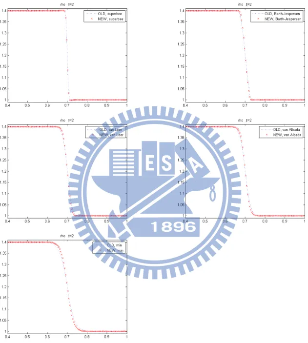
In this example, we compute the approximate solution at final time t=2, and use 200 grids points. Figure 4.1 shows the density, computing by the NEW and the OLD

central-upwind schemes. OLD central-upwind schemes is in (2.16) with the anti-diffusion term q_j+1

2 = 0. From those graphs, we know the NEW schemes have less dissipation than

the OLD schemes. Those solutions are especially close by the superbee limiters. The difference in the results still clearly visible by else limiters and the difference especially large in minmod limiters. Then we use NEW central-upwind schemes to compare five kinds of limiters in Figure 4.2. Numerical results show that superbee limiters achieve a better resolution but minmod limiters produce numerical dissipation larger than else limiters.

Example 2: Stationary contact wave and traveling shock and rarefaction

(ρ, u, p)(x, 0) =    (1, − 19.59745, 1000), x < 0.8 (1, − 19.59745, 0.01), x > 0.8

In this example, we use the 200 grids points on interval [0,1] and compute the solution at final time t=0.012. The computed density is plotted in Figure 4.3. The reference solution is obtained by the NEW second-order semi-discrete central-upwind scheme with 2400 grid points and plotted in Figure 4.4. Two graphs show superbee limiters with less dissipation in the neighborhood of the contact wave because the slope is sharper by using superbee limiters. Example 3 (ρ, u, p)(x, 0) =          (3.857143, − 0.920279, 10.33333), x < 0 (1 + ε sin 5x,−3.549648 , 1.00000), 0 < x < 10 (1.000000, − 3.549648, 1.00000), x≥ 10

This example is taken from [5] that corresponds to density perturbation running left-ward into stationary of Mach number 3. In this example, we computed the solution at final time t=2 and take ε = 0.2. The five solutions by the NEW second-order central-upwind schemes are obtained over interval (-15,15) with ∆x = 1

80. Figure 4.5 shows that

superbee limited solution has superiority of solution. The slope is least by using minmod limiters, so minmod limited solution exhibits excessive dissipation.

Example 4: Shock tube problem (ρ, u, p)(x, 0) =    (1.0, 0.0, 1), x < 0.5, (0.125, 0.0, 0.1), x > 0.5,

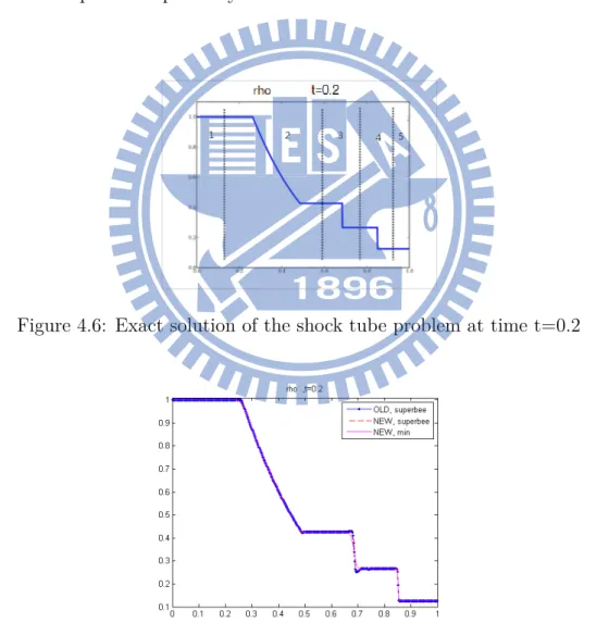
The exact solution of shock tube problem consists of rarefaction wave, shock wave, and contact discontinuity plotted in Figure 4.6 (see in [14, 16]). The computation of exact solution can be obtained in [16]. We compute the solution at final time t=0.2 and use the 400 grids points on interval [0, 1]. And we use the OLD central-upwind schemes with superbee limiters and NEW central-upwind schemes with superbee, and minmod limiters for this problem, respectively. As in Figures 4.7 and 4.8, OLD and NEW central-upwind schemes with superbee limiters have less numerical dissipation than one with minmod limiters. However, they produce a large oscillatory than ones with minmod limiters.

Example 5: Burgers’ equation

In this example, we consider the inviscid Burgers’ equation

ut+ ( 1 2u 2₎ x = 0, where u(x, 0) =    1, 0 < x < 1 , 0, otherwise. The exact solution of this example

u(x, t) =                0, x < 0, x/t, 0 < x < t, 1, t < x < 1 + t₂, 0, x > 1 + t₂, for t_{≤ 2, and} u(x, t) =          0, x < 0 , x/t, 0 < x <√2t, 0, √2t < x,

for t≥ 2.

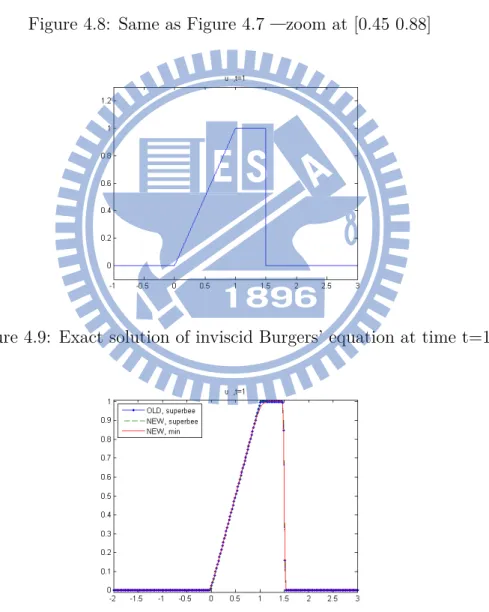
We computed the solution at final time t=1 and used the uniform grid with ∆x = 1/50. In Figures 4.10 and 4.11, we show the results obtained by the OLD central-upwind schemes with superbee limiters and NEW central-upwind schemes with superbee, and minmod limiters. And we plot the exact solution at t=1 as in Figure 4.9. From these graphs, they show that the new superbee limiters have less numerical dissipation than old superbee limiters.

From these examples, the superbee, Barth-Jespersen, van Leer and van Albada limited solution have less numerical dissipation but have oscillatory and perturbation for some cases. This is why minmod limiters is usuaully used.

Concluding Remarks:

In this thesis, we use new semidiscrete upwind-central schemes with anti-diffusion to reduce the numerical dissipation for hyperbolic conservation laws [6]. We modify the slope limiters at reconstruction step, choose the same limiters at projection step, and compute approximate solutions. The numerical results present that superbee limiter solution has least numerical dissipation but minmod limiter solution exhibits excessive dissipation.

For the future work, we will study the case when using different slope limiters at reconstruction and projection steps. We also will compare these resulting schemes to find one which has less numerical dissipation effectively. Furthermore, we can extend the study in one dimension to two dimension which is expected to be more complicated.

Figure 4.1: Example 1 computed by the NEW and OLD second-order schemes with same spatial grid

Figure 4.2: Example 1 computed by the NEW second-order schemes with five kinds of limiters

Figure 4.3: Example 2 computed by the NEW second-order schemes with five kinds of limiters and zoom at [0.67:0.88]

Figure 4.5: Example 3 computed by the NEW second-order schemes with five kinds of limiters

Figure 4.6: Exact solution of the shock tube problem at time t=0.2

Figure 4.7: Example 4 computed by the OLD and NEW second-order schemes at time t=0.2

Figure 4.8: Same as Figure 4.7 —zoom at [0.45 0.88]

Figure 4.9: Exact solution of inviscid Burgers’ equation at time t=1

Figure 4.10: Example 5 computed by the OLD and NEW second-order schemes at time t=1

References

[1] Francois Bouchut, An introduction to finite volume methods for hyperbolic conserva-tion laws, ESAIM Proc., 15 (2005), pp. 1–17.

[2] Steve Bryson, Alexander Kurganov, Doron Levy, and Guergana Petrova, Semi-discrete central-upwind schemes with reduced dissipation for Hamilton-Jacobi equa-tions, IMA J. Numer. Anal. 25 (2005), pp. 113–138.

[3] Steve Bryson and Doron Levy, High-order semi-discrete central-upwind schemes for multi-dimensional Hamilton-Jacobi equations, J. Comput. Phys. 189 (2003), pp. 63–87.

[4] Marcus Calhoun-Lopez and Max D. Gunzburger, A finite element, multiresolution viscosity method for hyperbolic conservation laws, SIAM J. Numer. Anal. 43 (2005), pp. 1988–2011.

[5] Smadar Karni, Alexander Kurganov, and Guergana Petrova, A smoothness indicator for adaptive algorithms for hyperbolic systems, J. Comput. Phys., 178 (2002), pp. 323–341.

[6] Alexander Kurganov and Chi-Tien Lin, On the reduction of numerical dissipation in central-upwind schemes, Commun. Comput. Phys. 2 (2007), pp. 141–163.

[7] Alexander Kurganov, Sebastian Noelle, and Guergana Petrova, Semidiscrete central-upwind schemes for hyperbolic conservation laws and Hamilton-Jacobi equation, SIAM J. Sci. Comput. 23 (2001), pp. 707–740.

[8] Randall J LeVeque, Numerical methods for conservation laws, Birkhäuser Basel, 1992.

[9] , Nonlinear conservation laws and finite volume methods, Springer Berlin Heidelberg, 1998.

[10] , Finite-volume methods for hyperbolic problems, Cambridge University, 2002.

[11] Knut-Andreas Lie and Sebastian Noelle, On the artificial compression method for second-order nonoscillatory central difference schemes for systems of conservation laws, SIAM J. Sci. Comput. 24 (2003), pp. 1157–1174.

[12] Haim Nessyahu and Eitan Tadmor, Nonoscillatory central differencing for hyperbolic conservation laws, J. Comput. Phys. 87 (1990), pp. 408–463.

[13] Rodolfo R. Rosales, Conservation laws in continuum modeling, MIT, 2001.

[14] Gary A Sod, A survey of several finite difference methods for systems of nonlinear hyperbolic conservation laws, J. Computational Phys. 27 (1978), pp. 1–31.

[15] P. K. Sweby, High resolution schemes using flux limiters for hyperbolic conservation laws, SIAM J. Numer. Anal. 21 (1984), pp. 995–1011.

[16] Eleuterio F Toro, Riemann solvers and numerical methods for fluid dynamics, Springer; 3rd edition, 2009.

[17] Jin-chao Xu and Lung-an Ying, Convergence of an explicit upwind finite element method multi-dimensional conservation laws, J. Comput. Math. 19 (2001), pp. 87–100.