CBD Oriented Commuters’ Mode and Residential Location
Choices in an Urban Area with Surface Streets and Rail
Transit Lines
Chaug-Ing Hsu
1and Shwu-Ping Guo
2Abstract: This study formulates a commuters’ mode and route choice model as well as a households’ residential choice model on a two-dimensional space. The commuters’ mode and route choice model assumes that commuters select the mode and route alternative based on the least generalized travel cost. The households’ residential choice model is formulated to maximize households’ residential utilities subject to time and budget constraints. A simulation method is adopted to simulate household choice behavior and solve the households’ residential location choice model with two-dimensional decision variables to prevent aggregation bias. A case study for Taipei metropolitan area is illustrated to analyze the variations of residential location choices for households working in the central business district 共CBD兲 after different lines of Taipei Rapid Transit System are completed at various stages. Results indicate that 共1兲 there is increased attraction of households in cities of Taipei County such as Pan-Chiao, Chung-Ho, Yong-Her, and Hsin-Tien due to the completion of rail transit networks and共2兲 residential locations better served by rail transit lines attract more households; thereby, resulting in higher residential densities.
DOI: 10.1061/共ASCE兲0733-9488共2006兲132:4共235兲
CE Database subject headings: Residential location; Urban areas; Streets; Commute; Models; Spatial distribution; Rail transportation.
Introduction
Most residential location models in urban economic-related stud-ies are originated from Alonso’s location model 共Alonso 1964兲. That model assumes that all workplaces are concentrated in a highly compact central business district共CBD兲 on the side of city configurations. Commuters’ homes are continuously dispersed over the residential area surrounding the CBD. All commuters are employed at the CBD. Only homogeneous surface streets are as-sumed to be available on the side of transportation systems. Thus, the complicated two-dimensional city configuration can be sim-plified to a one-dimensional round city. Relevant studies include Higano and Orishimo共1990兲, Lund and Mokhtarian 共1993兲, Hi-gano 共1991兲, Shibusawa and Higano 共1995兲, and Shibusawa 共1997兲. The previous literature was based on the assumption of the round city configuration and approximated traffic networks by continuous surface streets. Therefore, these studies usually ne-glected the effects of rail transit networks on commuters’
residen-tial location choices. Traffic congestion is attributed mainly to the temporal concentration of trips in the city with concentrated workplaces. Yang et al.共1994兲 assumed that two kinds of trans-portation systems, dense surface streets, and a discrete rail transit network are concurrently applied to alleviate traffic congestion in urban areas. On rail transit networks, the schedule and the speed of trains are controlled and monitored by a central control center; thus, passengers can predict their on-board time and rail transit company can also maintain schedule adherence. On the contrary, driving automobiles on surface streets can take the advantage of accessibility door-to-door services.
Residential location choice models on conventional transpor-tation planning are based on traffic zones. Waddell共1993兲 devel-oped a nested logit model of workers’ choices of workplace, residence, and housing tenure under the assumption that choice of workplace was exogenously determined. Moreover, Eliasson and Mattsson 共2000兲 designed a model for integrated analysis of household location and travel choices by applying a nested logit model. Each household made a joint choice of location共zone and house type兲 and travel pattern 共trip frequencies, destination choices, and mode choices兲 so as to maximize utility subject to budget and time constraints. Martinez共1992兲 made a theoretical comparison of the bid-rent theory and the discrete-choice random-utility theory used in modeling urban land use. Watterson 共1993兲 recognized the relationship between urban spatial form and urban transportation system by analyzing several variables such as transportation facility investments, demand management measures, and land-use controls. Hunt and Simmonds共1993兲 con-structed an integrated land-use and transport framework with the concept of market and supply-demand analysis. Hunt et al.共2004兲 introduced the household allocation module of OREGON2 model with selection probabilities determined using logit models and sampling distributions. Wong et al.共2004兲 formulated a combined 1
Professor, Dept. of Transportation Technology and Management, National Chiao Tung Univ., Hsinchu 30010, Taiwan, Republic of China. E-mail: [email protected]
2
Assistant Professor, Dept. of Logistics Management, Leader Univ., Tainan 709, Taiwan, Republic of China. E-mail: spguo@ mail.leader.edu.tw
Note. Discussion open until May 1, 2007. Separate discussions must be submitted for individual papers. To extend the closing date by one month, a written request must be filed with the ASCE Managing Editor. The manuscript for this paper was submitted for review and possible publication on May 3, 2005; approved on February 13, 2006. This paper is part of the Journal of Urban Planning and Development, Vol. 132, No. 4, December 1, 2006. ©ASCE, ISSN 0733-9488/2006/4-235–246/ $25.00.
distribution and assignment model for travelers’ choices for re-gional activity centers using a flow- and location-dependent trans-portation cost function. Hsu and Guo共2001兲 formulated a model integrating households’ residential-mode choice and residential distribution in a metropolitan area with surface streets and rail transit networks using continuous analytical approaches and mathematical programming methods. The previous studies must collect extensive data about households, houses, land rents and transportation networks. Comprehensive and time-consuming programs are also required to obtain the equilibrium solution. The extension of those models to long-term time dependent analyses becomes a very complicated problem.
In practice, a household’s residential location is determined by the residential utility of each location rather than traffic zones confined by administrative districts or census tracts. Thus, this study divides the study area into numerous equal-sized grids and allocates each household to a specific coordinate to scan the dis-tribution of households in the study area. In addition, most studies involving the choices of households’ residential locations in the metropolitan area of Taiwan constructed an allocation model which grouped the households into several groups according to factors such as income, automobile ownership, and the number of household members, such as in Feng and Yang 共1989兲. Those studies also assigned each group of households to a traffic zone by using conventional land use models. In this manner, these models neglected the heterogeneity among individual households of the same group and, therefore, aggregation bias could not be prevented. For these reasons, this study applies a sampling method to collect data of households’ attributes such as working hours, hourly salary, and living area so as to estimate the distri-bution of households’ attributes. Accordingly, a simulation method is adopted to generate individual households with differ-ent attributes so as to describe an individual household’s behavior more accurately.
Owing to heavy traffic at peak periods, rail transit with high capacities is normally implemented to streamline the transport of commuters from homes to their workplaces in the metropolitan area. In this study, two sequential models are constructed on a two-dimensional space to analyze the household distribution in a monocentric city with surface streets and rail transit lines. Surface streets are assumed herein to be dense networks and rail transit lines are assumed to be discrete networks. A mathematical pro-gramming model for individual household’s optimal residential locations is formulated by maximizing residential utility subject to the household’s budget and time constraints. Factors determin-ing household’s residential utilities are work time, leisure time, commuting time and cost, and the residual of disposable income deducted by the rent of floor areas and the commuting cost. In addition, the commuters’ route and mode choice model is used to determine the commuting times from each of all residential loca-tions to the CBD. Commuters in this route and mode choice model are assumed to either travel straight along dense surface streets to CBD or travel along dense surface streets to a rail transit station and, then, ride to the CBD by rail transit depending on which one has the least generalized travel cost. The interaction between the commuters’ mode and route choice and household’s residential location choice is established by solving two models iteratively in each time interval. The time intervals here are time spans between different rail transit lines are completed. In the meantime, the total number of immigrating households in each time interval is assumed to be exogenous.
Commuters’ Mode and Route Choices
This study applies analytical methods to construct a static com-muters’ mode and route choice model. Commuters are assumed to have two mode and route alternatives. That is, a commuter can either travel straight along dense surface streets to CBD or travel along dense surface streets to a rail transit station and, then, ride a train to the CBD. The proposed model not only defines the generalized travel cost as the weighted sum of travel time and travel cost, but also derives the travel time and travel cost of each alternative from residential locations to the CBD under flow-independent assumption of travel costs and travel times. Commut-ers are assumed to maximize their utilities and to choose the alternative with the least generalized travel cost. On the side of surface streets, let B⬘represent the two-dimensional study area, as well as X and O denote the coordinate 共x1, x2兲 of a residential
location and the coordinate 共o1, o2兲 of the CBD, respectively.
Then, the travel distance on surface streets, D共X,O兲, from resi-dential location X to the CBD O is expressed as the sum of the horizontal and vertical distances between the two coordinates as
D共X,O兲 = 兩x1− o1兩 + 兩x2− o2兩 共x1,x2兲 苸 B⬘ 共1兲
The distance defined by Eq.共1兲 is usually called Manhattan dis-tance. In addition, letvLand fLrepresent the average travel speed
and the fuel cost per kilometer on surface streets, respectively. Let cOdenote the parking cost at CBD per work trip. Parameter ss is
a constant over B⬘and stands for the scale which transforms the grid distance into the actual distance on surface streets for the study area. The round-trip travel time, TL共X兲, and the round-trip travel cost, CL共X兲, from residential location X to the CBD O via
surface streets can then be expressed as the following equations, respectively,
TL共X兲 = 2D共X,O兲ss/vL ∀ 共x1,x2兲 苸 B⬘ 共2兲
CL共X兲 = 2D共X,O兲ssfL+ cO ∀ 共x1,x2兲 苸 B⬘ 共3兲 Eqs.共2兲 and 共3兲 assume that route and mode choices to and from the CBD are completely symmetric. Namely, there is no round traveling from office for shop and then return for home. This study assumed surface streets to be dense networks and rail transit lines to be discrete networks. The major advantage of assuming surface streets to be dense networks is to avoid time-consuming data collection for surface streets. Based on a long-term planning perspective, this study adopts the average values to represent travel speed and fuel cost per kilometer on surface streets. Mean-while, rail transit networks are constructed in different phases. This approach enables the relative advantage on mobility of rail transit over time to be captured and a reasonable result to be obtained though the assumption about surface streets is unrealistic from the perspective of the real world. On the side of rail transit lines, let M denote the number of rail transit lines and Jirepresent
the number of stations on the ith rail transit line where i = 1,2 , . . . , M. The coordinate共y1, y2兲 of the jth station on the ith
rail transit line is represented by Sijwhere j = 1,2 , . . . , Ji. Then, the
travel distance on surface streets, D共X,Sij兲, from each residential
location X to station Sij can be formulated by
D共X,Sij兲 = 兩x1− y1兩 + 兩x2− y2兩 for i = 1,2, ... ,M;
j = 1,2, . . . ,Ji; 共x1,x2兲 苸 B⬘ 共4兲 Let L共Sij, O兲 represent the distance from the rail transit station Sij
to the CBD,vTi stand for the average running speed of trains on
the ith rail transit line, wSijdenote the total stop delay from station
Sijto the CBD, hirepresent the average headway of the ith rail
transit line, fSijstand for the fare from station Sijto the CBD, and
cSij denote the average parking cost at station Sij. Then, the
roundtrip travel time and the roundtrip travel cost from residential location X to CBD O by traveling along surface streets and then transferring to rail transit line i at station Sijcan be formulated by
the following equations, respectively, TT共X,Sij兲 = 2D共X,Sij兲ss/vL+ 2wS ij+ hi+ 2L共Sij,O兲/vTi for i = 1,2, . . . , M and j = 1,2, . . . ,Ji; ∀ 共x1,x2兲 苸 B⬘ 共5兲 CT共X,Sij兲 = 2D共X,Sij兲ss · fL+ cSij+ 2fSij for i = 1,2, . . . , M and j = 1,2, . . . ,Ji; ∀ 共x1,x2兲 苸 B⬘ 共6兲
Let denote the value of time and gOdenote the average
gener-alized travel cost from stations at CBD to the workplace. Then, the generalized travel cost from residential location X to the CBD by traveling on surface streets, ZL共X兲, can be expressed as
ZL共X兲 = · TL共X兲 + CL共X兲 ∀ 共x1,x2兲 苸 B⬘ 共7兲
For the generalized travel cost from residential location X to the CBD by traveling along surface streets and then transferring to rail transit at station Sij, ZT共X,Sij兲, can be formulated by
ZT共X,Sij兲 = · TT共X,Sij兲 + CT共X,Sij兲 + gO
for i = 1,2, . . . , M ; j = 1,2, . . . ,Ji; 共x1,x2兲 苸 B⬘
共8兲 Because rail transit lines cannot provide door-to-door transport service, commuters traveling along surface streets and then trans-ferring to rail transit must spend more time and cost on walking or shuttle between the station in the CBD and workplaces. This situation is implied in this model with the parameter gO.
Let G*= min兵Z
L, ZT其 denote the least generalized travel cost.
Restated, the least travel time T*, the least travel cost C*and the
optimal route and mode choice, which are decision variables in the model, can be determined by comparing the values of ZLand
ZT in Eqs. 共7兲 and 共8兲 and then choosing the one with the least
value.
Household’s Residential Location Choice Residential Location Choice Model
All commuters in a household are assumed to work at workplaces within the CBD in this study. Herein, a household’s residential location choice model is constructed to maximize the household’s residential utility. Factors influencing the ith household’s utility at residential location X include the household’s total work time tWi,
the household’s total leisure time tLi, round-trip commuting cost
C*共X兲 and roundtrip commuting time T*共X兲 from residential
loca-tion X to the CBD, the residual of disposable income deducted the rent of floor areas and the commuting cost, Ii, and the existing number of households at residential location X after i-1 house-holds are allocated to the study area HHi−1共X兲. This study defines
T
¯ as the total time constraint for one person and supposes that the study period is one month measured by hours; that is, 720 h. Let wibe the ith household’s average hourly salary, RH共X兲 represent
the rent per area unit共e.g., per pyng, which is a measurement unit of area in Taiwan and is equal to an area of 0.3025 m2兲 at
resi-dential location X, lHi represent the ith household’s residential
floor area, t¯ denote the commuter’s average monthly commuting frequency, and n¯ denote the average number of commuters in a household. Then, the model for the ith household’s residential location choice under time constraint and income budget can be formulated by
max Ui= U共tLi,C*,T*,Ii,HHi−1X兲 共9兲
s.t ¯ · Tn ¯ − tWi− tLi− n¯ · T*共X兲 · t¯ = 0 共10兲
wi· tWi− Ii− RH共X兲 · lHi− C*共X兲 · t¯ · n¯ = 0 共11兲
共x1,x2兲 苸 B⬘ 共12兲
Eq.共9兲 is the ith household’s residential utility function. Eqs. 共10兲 and共11兲 are the total time constraint and the budget constraint for a household, respectively. The chosen residential location con-fined to the study area B⬘ is specified by Eq. 共12兲. Similar to investigations such as Lund and Mokhtarian 共1993兲, Shibusawa and Higano共1995兲, and Eliasson and Mattsson 共2000兲, this study analyzes how the household’s leisure time, commuting cost, and commuting time influence the residential utility. Moreover, the residual of disposable income deducted the rent of floor areas and the commuting cost markedly influences the household’s con-sumption power. The number of households at each residential location determines the intensity of traffic congestion. Owing to the assumption of monocentric urban configuration, commuting households, who depart their homes to workplaces, cause conges-tion on the routes between their residences and workplaces. This study explores commuters’ mode and residential location choice from the perspective of long term planning. To simplify network representation problem, this study represents surface streets as a dense grid network using continuous network approach by New-ell 共1980兲 and Vaughan 共1987兲. This study uses the number of household at each residential location to approximately explain the effect of surface street congestion at the location while not dealing with detailed traffic assignment problem for surface street, which is usually regarded as short term operational prob-lem. Additionally, the degree of air pollution and noise is closely related to the intensity of traffic congestion. Notably, the living quality of a residential location decreases with an increase of the number of households when the area at each residential location cannot be further expanded. That is, open spaces for parks, edu-cational facilities, and other resorts become relatively insufficient, thereby degrading quality of life. In response to these factors, household’s disposable income and the number of households at each residential location are considered in the residential utility function in this model. This study assumes factors such as com-muting time, comcom-muting costs, and leisure time may incur inter-active and nonlinear effects on the commuters’ residential utility, and formulates the residential utility function by applying a mul-tiplicative functional form as
Ui= tLi␣1C
*共X兲␣2T*共X兲␣3I
i
␣4HH
i−1共X兲␣5 共13兲
where␣1,␣2,␣3, ␣4, and␣5⫽parameters.
The main focus of this study is on exploring mode/route and residential location choices of commuting households, due to the completion of rail transit lines. To focus on the key issues, vari-ables such as work hour, wage, and lot size are assumed to be exogenous and thus are assigned randomly. When rail transit lines
operate sequentially, commuting time and cost from each residen-tial location to the workplace gradually change. The optimal residential location of individual households thus might vary accordingly. Further, when households choose residential loca-tions with different rents, their choices depend on their biding capability in terms of disposal incomes. Based on these consider-ations, this study adopts commuting time, commuting cost, leisure time, rent and residual of disposable income after deducting rent and commuting costs in the residential utility function.
Simulation Method
Decision variables of the household’s residential location choice model, as formulated by Eqs. 共9兲–共12兲, are coordinates of two-dimensional residential locations for households. The commuting cost and the commuting time of each commuter in the residential location choice model are varied as the chosen residential location and the optimal mode choice change. Generally, conventional methods for solving mathematical programming model are inap-propriate for solving problems such as the one with the above-mentioned two-dimensional decision variables. Therefore, the Monte Carlo simulation method is proposed herein to construct a stochastic simulation model for determining the optimal residen-tial location of each household. Households with different at-tributes are generated sequentially by the next event incrementing method and, then, allocated to the optimal residential location. Further, the construction of rail transit networks is very time con-suming and is usually implemented at several construction stages. Effects of rail transit networks on commuters’ mode and route choices and household’s residential location choice are also pro-gressive. To differentiate the various lag effects of incremental rail transit lines completed at various stages, this study divides the study period into several time intervals. In each time interval, there are different numbers of rail transit lines completed. The commuter’s mode and route choices model and household’s resi-dential choice model are then solved, respectively, for time inter-vals with the increasing numbers of completed rail transit lines.
Household’s Attribute Generator
The household’s attributes in this model include the monthly working hours, average hourly salary, and required residential floor area. This study postulates that these three types of attributes follow the triangular distribution. Reasons for selecting triangular distribution functions herein to simulate individual household’s attributes are as follows. First, the function form of triangular distribution is bounded, meaning that extreme values are avoided and attribute values are confined to a reasonable range. Second, compared to a truncated normal distribution, the function form of the triangular distribution is linear and thus the inverse of its cumulative distribution is easily derived. The inverse is signifi-cant in simulation models, because a random number generator generally is designed to obtain a positive real number rather than a statistic representing household’s attributes. The inverse func-tion is crucial to converting the random number into an appropri-ate statistic. However, the normal distribution contains an integral term, making its cumulative distribution and inverse complicated to compute. To simplify the problem solving procedure, this study adopts the triangular distribution to explain households’ at-tributes. Moreover, the generalized exponential family of distributions may be used to describe income distribution and generalized exponential family distributions include such useful distributions as normal, beta, generalized normal, generalized
beta, etc.共Bakker and Creedy 2000兲. The triangular distribution formulated below is the special case of Beta distribution for a = 0 and b = 1共Law and Kelton 1982兲.
The triangular distribution is formulated by Y⬃triang共a,b,c兲, where a⬍c⬍b and c is the mode of the sample. In addition, Y⬘⬃triang关0,1,共c−a兲/共b−a兲兴 can be obtained by letting Y⬘=共Y −a兲/共b−a兲. Let c⬘=共c−a兲/共b−a兲, then, by referring to Law and Kelton 共1982兲, the distribution function is easily in-verted to obtain as shown for 0ⱕuⱕ1, by
Y⬘= F−1共u兲 =
再
共c⬘u兲1/2 if 0ⱕ u ⱕ c⬘
1 −关共1 − c⬘兲共1 − u兲兴1/2 if c⬘ⱕ u ⱕ 1 共14兲 Correspondingly, according to Law and Kelton 共1982兲, the fol-lowing inverse-transform algorithm can be stated for generating a household’s attributes:
1. Generate a random variable U⬃U共0,1兲 by applying linear congruential generators.
2. If Uⱕc⬘, set Y⬘=共c⬘U兲1/2; otherwise, set Y⬘= 1 −关共1−c⬘兲共1
− U兲兴1/2.
3. Set the household’s attribute as Y = a +共b−a兲Y⬘and return. This study adopts the linear congruential generators to generate a random variable following the uniform distribution, i.e., U⬃U共0,1兲. This method recursively generates an integer se-quence, Z1, Z2, . . . , Zi−1, Zi, . . . in
Zi=共aZi−1+ c兲mod m 共15兲
where the modulus m, multiplier a, increment c, and seed Z0are
nonnegative.
The triangular distribution is similar to the uniform distribu-tion except there is an intercepdistribu-tion, the mode of sample, in the triangular distribution function. The modes of triangular distribu-tions are estimated, respectively, by using the average values of working hours, hourly salary, and required residential floor area of the representative households; whereas the upper bounds and lower bounds of triangular distributions are estimated, respec-tively, by employing the maximal and minimal values of those of the households.
Processes of the Simulation Program
The simulation program in this study is written by C language. The basic concepts, assumptions and considerations of each phase in the program are explained as follows.
Phase 1: Set initial values of parameters a, c, m, and Z0for the
random number generator. Initialize the parameters of the house-hold’s attribute generator. These include three classes of param-eters. Parameters Ta, Tb, and Tc represent, respectively, the minimal value, the mode, and the maximal value for the triangu-lar distribution of monthly working hours. Parameters Wa, Wb, and Wc signify the minimal value, the mode, and the maximal value for the triangular distribution of the average hourly salary, respectively. Parameters La, Lb, and Lc denote the minimal value, the mode and the maximal value for the triangular distribution of the required residential area, respectively. The basic requirement of disposable income deducted the rent of floor areas and com-muting cost is assigned to maintain the living standard. The basic requirement of the leisure time defined as the time excluding the working time and commuting time is assigned in this program as well. Set initial time interval k = 1.
Phase 2: Read data related to parameters of the commuters’ mode and route choice model such as average travel speed and fuel cost per kilometer on surface streets, average parking cost per
work trip at CBD, average running speed and fare on rail transit networks, etc. Solve the commuters’ mode and route choice model in Sec. 2 to obtain the commuting cost and commuting time from each residential location to the CBD in time interval k and read the obtained data. Read data about monthly rent per pyng at each residential location. The monthly rent at each resi-dential location is measured by the monthly monetary cost re-quired to recover the real estate price per pyng. The interest rate and the recovery period are assumed to be 6% and 35 years, respectively.
Phase 3: Generate, randomly, three attributes, i.e., the monthly working time, the average hourly salary and the residential area according to the processes in Sec. 3.2.1 for each household in time interval k. The total number of households in the time inter-val k equals the total number of households in the previous time interval plus the net number of immigrating households in the time interval k.
Phase 4: Calibrate the values of parameters in the residential utility function by using simulated methods for time interval k = 1. Collect data about the number of households at the begin-ning and the end of time interval k = 1 at each residential location in the study area. Steps in the calibration process include: • Initialize several alternative sets of values for parameters
␣1,␣2, ␣3,␣4, and␣5.
• Input simulated household attributes obtained in Phase 3. Solve, iteratively, individual household’s residential location choice model as many times as the total number of households according to the principles described in Phase 5.
• Compare the model number of households with the actual number of households at each residential location by defining the deviation as兩model number−actual number兩/actual number. Choose the maximal deviation among those of all residential locations to represent the performance of model calibrated results.
• Apply the minimal of maximal principle for the deviations of models using alternative parameter value sets to determine an appropriate set of values for parameters ␣1,␣2,␣3, ␣4,
and␣5.
Phase 5: Use parameters calibrated in Phase 4 and solve the household’s residential location model of Eqs.共9兲–共12兲 to identify the residential location with the maximal residential utility for a household. If the optimal residential location for a household is not unique, then an arbitrary decision is assumed for the house-hold. Then, the number of households at each residential location is updated. On the other hand, if the residual of disposable income deducted the rent and commuting cost for the household allocated to the optimal location is less than the basic requirement, then the allocation of this household is negated. Similarly, if household’s leisure time does not exceed the basic requirement, the allocation of this household is negated as well. Compare the updated de-mand and supply of residential areas at each residential site. If the capacity of individual residential site is saturated, then the resi-dential site is unavailable for allocating households any more.
Phase 6: If the next time interval does not exceed the study period, update data about rail transit networks and households and solve the models by setting time interval to the next time interval, that is, k = k + 1 and repeating Phases 2, 3, and 5. Otherwise, if the next time interval exceeds the study period, output the household density, average income, and average leisure time at each residen-tial location for all time intervals in the study area.
This study defines time intervals as time spans between the completions of different rail transit lines. A completed transit line increases the accessibility of the area serviced, thus influencing
rent of floor areas. Rent of floor areas at each residential location is also a critical influence on individual household’s residential choice. In this study, rent per pyng, RH共X兲, at residential location
X which appears in individual household’s budget constraint, namely, Eq.共11兲, is further assumed to be a linear function of the number of household’s in the previous time interval. That is, due to the households’ bid-rent effect, rent per pyng at each residential location rises with increased number of households choosing to reside at that location. To elucidate the interaction between rent of floor areas and number of biding households, this study assumes the linear equation of rent per pyng RHt共X兲 in time interval t to be the following equation and adjusts its value according to the num-ber of households HHi−1共X兲 at residential location X at the end of
time interval t-1: RH
t共X兲 = R H
t−1共X兲共1 + ␥兲 共16兲
Symbols t and t − 1, respectively, represent time intervals t and t − 1. Moreover, parameter␥⫽an adjustment factor of rent of floor areas. According to the study of Yuan共2003兲, the determination of land value variation in Taiwan involves substantial efforts in field survey and land policy from a time-consuming political pro-cess. The bidding effect of households on land rent exists and is demonstrated by many studies such as Alonso共1972兲 and Ching and Fu 共2003兲. This study focuses on the relationship between land price and the number of bidding households using simplified equations as Eq. 共16兲 and the following equation, where 1,2,
3, and 4 are assumed to be 0.015, 0.030, 0.045, and 0.060,
respectively, in the case study to show the increasing bidding effects of household numbers on land rent:
␥ =
冦
1 if 0⬍ 关HHt共X兲 − HHt−1共X兲兴 ⱕ 20 2 if 20⬍ 关HHt共X兲 − HHt−1共X兲兴 ⱕ 40 3 if 40⬍ 关HHt共X兲 − HHt−1共X兲兴 ⱕ 60 4 if 61⬍ 关HHt共X兲 − HHt−1共X兲兴 共17兲 Illustrative ExampleData for Commuters’ Mode and Route Choices
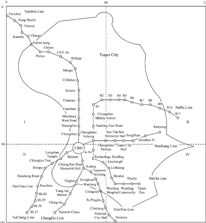
This study demonstrates the application of the proposed model by presenting a case study with a metropolitan area covered by the Taipei Rapid Transit System, as illustrated in Fig. 1. The study area, which is represented by a two-dimensional coordinate sys-tem, is divided into 120⫻150=18,000 equal-sized grids. Surface streets are approximated by dense networks and assumed to be homogeneous in the study area. The completion dates of other rail transit lines are:共1兲 Nankang Line in 2001; 共2兲 Panchiao Line in 2005; and共3兲 Nehu Line in 2009. The period from 1997 to 1999 is treated as time interval one. The period from 1999 to the completion date of Nankang Line is treated as time interval two. The period between the completion date of Nankang Line and that of Panchiao Line is treated as time interval three. Finally, the period between the completion date of Panchiao Line and that of Nehu Line is treated as time interval four. The numbers of immi-grating households during four time intervals are estimated as 495,342, 208,566, 347,608, and 391,059, respectively. The illus-trated example is used to analyze the residential location choices of households working in the region of the Taipei Central Rail Station 共the center of CBD兲 after different lines of the Taipei Rapid Transit System are completed at various stages in the fu-ture. Interactions between transportation systems and land use
systems are established by iteratively solving the commuters’ mode and route choice model and the households’ residential lo-cation choice model. Although this study is assumed to be a monocentric city configuration, subsequent studies can extend it to multicentric city configuration by similar methods. In the com-muters’ route and mode choices model, data about surface streets include the average travel speed on surface streets, the fuel cost per kilometer on surface streets and the expected parking cost per work trip on the CBD. These data are estimated from relevant studies to be 32.5 km/ h, NT$ 3.8/ km and NT$240共one U.S. dol-lar is equal to approximately NT$33兲, respectively.
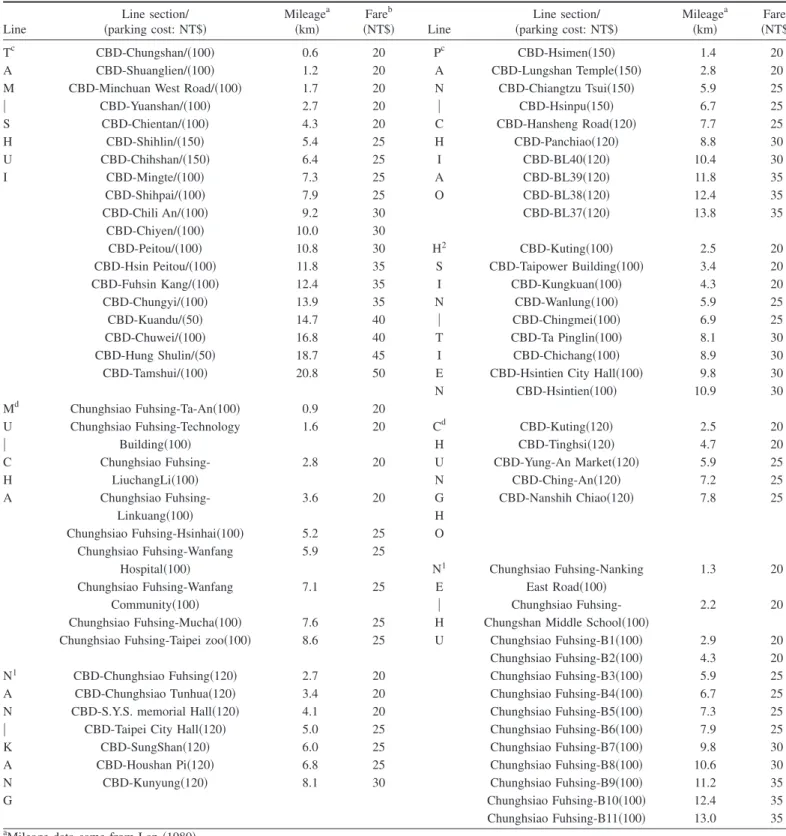
Data about the Taipei Rapid Transit System such as the net-work configuration, headway and average running speed of each line, fare and distance from each station to the CBD, expected
parking cost per trip and average stop delay at each station are accumulated from the official reports of the Department of Rapid Transit Systems of Taipei City Government and other investiga-tions and are summarized in Table 1. Other data such as the expected generalized travel cost from stations in the CBD to workplaces, the value of time and the scale of the grid are as-sumed to be NT$ 60, NT$ 4 / min, and 0.2 km, respectively. More-over, this study assumes that each station has enough parking facilities.
Data for Household’s Residential Location Choice
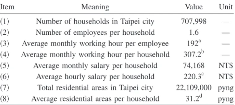
The household’s total working time, average salary and average residential area shown in Table 2 come primarily from The
Sta-Fig. 1. Diagram of the study area
Table 1. Mileage, Fare, and Parking Cost on Taipei Rapid Transit System Line
Line section/
共parking cost: NT$兲 Mileage a
共km兲 Fare b
共NT$兲 Line
Line section/
共parking cost: NT$兲 Mileage a
共km兲 Fare b 共NT$兲
Tc CBD-Chungshan/共100兲 0.6 20 Pc CBD-Hsimen共150兲 1.4 20
A CBD-Shuanglien/共100兲 1.2 20 A CBD-Lungshan Temple共150兲 2.8 20
M CBD-Minchuan West Road/共100兲 1.7 20 N CBD-Chiangtzu Tsui共150兲 5.9 25
兩 CBD-Yuanshan/共100兲 2.7 20 兩 CBD-Hsinpu共150兲 6.7 25
S CBD-Chientan/共100兲 4.3 20 C CBD-Hansheng Road共120兲 7.7 25
H CBD-Shihlin/共150兲 5.4 25 H CBD-Panchiao共120兲 8.8 30 U CBD-Chihshan/共150兲 6.4 25 I CBD-BL40共120兲 10.4 30 I CBD-Mingte/共100兲 7.3 25 A CBD-BL39共120兲 11.8 35 CBD-Shihpai/共100兲 7.9 25 O CBD-BL38共120兲 12.4 35 CBD-Chili An/共100兲 9.2 30 CBD-BL37共120兲 13.8 35 CBD-Chiyen/共100兲 10.0 30 CBD-Peitou/共100兲 10.8 30 H2 CBD-Kuting共100兲 2.5 20
CBD-Hsin Peitou/共100兲 11.8 35 S CBD-Taipower Building共100兲 3.4 20
CBD-Fuhsin Kang/共100兲 12.4 35 I CBD-Kungkuan共100兲 4.3 20
CBD-Chungyi/共100兲 13.9 35 N CBD-Wanlung共100兲 5.9 25
CBD-Kuandu/共50兲 14.7 40 兩 CBD-Chingmei共100兲 6.9 25
CBD-Chuwei/共100兲 16.8 40 T CBD-Ta Pinglin共100兲 8.1 30
CBD-Hung Shulin/共50兲 18.7 45 I CBD-Chichang共100兲 8.9 30
CBD-Tamshui/共100兲 20.8 50 E CBD-Hsintien City Hall共100兲 9.8 30
N CBD-Hsintien共100兲 10.9 30
Md Chunghsiao Fuhsing-Ta-An共100兲 0.9 20
U Chunghsiao Fuhsing-Technology 1.6 20 Cd CBD-Kuting共120兲 2.5 20
兩 Building共100兲 H CBD-Tinghsi共120兲 4.7 20
C Chunghsiao Fuhsing- 2.8 20 U CBD-Yung-An Market共120兲 5.9 25
H LiuchangLi共100兲 N CBD-Ching-An共120兲 7.2 25
A Chunghsiao Fuhsing- 3.6 20 G CBD-Nanshih Chiao共120兲 7.8 25
Linkuang共100兲 H
Chunghsiao Fuhsing-Hsinhai共100兲 5.2 25 O Chunghsiao Fuhsing-Wanfang 5.9 25
Hospital共100兲 N1 Chunghsiao Fuhsing-Nanking 1.3 20
Chunghsiao Fuhsing-Wanfang 7.1 25 E East Road共100兲
Community共100兲 兩 Chunghsiao Fuhsing- 2.2 20
Chunghsiao Fuhsing-Mucha共100兲 7.6 25 H Chungshan Middle School共100兲
Chunghsiao Fuhsing-Taipei zoo共100兲 8.6 25 U Chunghsiao Fuhsing-B1共100兲 2.9 20 Chunghsiao Fuhsing-B2共100兲 4.3 20
N1 CBD-Chunghsiao Fuhsing共120兲 2.7 20 Chunghsiao Fuhsing-B3共100兲 5.9 25
A CBD-Chunghsiao Tunhua共120兲 3.4 20 Chunghsiao Fuhsing-B4共100兲 6.7 25
N CBD-S.Y.S. memorial Hall共120兲 4.1 20 Chunghsiao Fuhsing-B5共100兲 7.3 25
兩 CBD-Taipei City Hall共120兲 5.0 25 Chunghsiao Fuhsing-B6共100兲 7.9 25
K CBD-SungShan共120兲 6.0 25 Chunghsiao Fuhsing-B7共100兲 9.8 30
A CBD-Houshan Pi共120兲 6.8 25 Chunghsiao Fuhsing-B8共100兲 10.6 30
N CBD-Kunyung共120兲 8.1 30 Chunghsiao Fuhsing-B9共100兲 11.2 35
G Chunghsiao Fuhsing-B10共100兲 12.4 35
Chunghsiao Fuhsing-B11共100兲 13.0 35 a
Mileage data came from Lan共1980兲. b
Fares are realistic data from official web site具http://www.trtc.com.tw典, and fares about uncompleted rail transit lines are estimated according to standard pricing rules adopted by the Taipei Rapid Transit Corporation.
c
Uncompleted rail transit line. Average operating speed, average headway, and average stop delay are assumed to be 33 km/ h, 5 min, and 30 s, respectively.
d
Average operating speeds, average headway, and average stop delays for Tamshui, Chungho, Hsintien, and Mucha Lines are 35 km/ h, 10 mins, 30 s, 33 km/ h, 5 min, 30 s, 33 km/ h, 5 min, 24 s, and 33 km/ h, 5 min, 30 s, respectively.
tistical Abstract of Taipei City共Department of Budget, Account-ing and Statistics 1997兲 and The Report on the Time Utilization Survey共DGBAS 1995兲 in Taiwan. The average monthly working hour, the average hourly salary and the average residential area in Table 2 are treated as sample modes of the three triangular distri-butions in Section 3.2.2. That is, they represent values for param-eters Tb, Wb, and Lb, respectively. The remaining six paramparam-eters Ta, Tc, Wa, Wc, La, and Lc are estimated to be 225 h, 345 h, NT$ 180, NT$ 325, 26 pyng, and 50 pyng, respectively. Data re-garding the real estate prices are accumulated from the House and Life magazine in Taiwan. Table 3 summarizes the data.
Result Analysis
Mode and Route Choices
The commuter’s mode and route choice model applied in the example not only estimates the least travel cost and travel time from each residential location to the CBD, but also determines the optimal mode choice for households who are living at each loca-tion of the study area and working in the CBD. Fig. 2 illustrates the optimal mode and route choice from each residential location to the CBD and the service area of each rail transit line after rail transit lines are totally completed; that is, in time interval four.
Commuters living in Area 1 and traveling to the CBD should drive a car via surface streets and then transfer to the Tamshui Line so as to minimize their generalized travel costs. Optimal transferring rail transit lines for commuters living in Areas 2, 3, 4, 5, 6, and 7 and traveling to the CBD are the Panchiao Line, Chungho Line, Hsintien Line, Mucha Line, Nankang Line, and Nehu Line, respectively. The optimal mode choice for commuters living in Area 8 is driving a car directly via surface streets to the CBD. The previous results indicate that commuters with longer travel distances between homes and CBD tend to use rail transit lines as their main commuting modes, whereas commuters with shorter travel distances tend to use car directly to the CBD via surface streets. Besides, the service areas of rail transit lines are not only resulted from the competition between rail transit net-works and surface streets but also from the competition between adjacent rail transit lines. For example, no rail transit line exists in the remote area between the east of the Tamshiu Line and the north of the Nehu Line; therefore, the service areas of these two lines are markedly large.
Figs. 3共a–c兲 illustrate, respectively, the equicommuting time 共unit: minute兲, equicommuting cost 共unit: NT$兲 and equi-generalized commuting cost共unit: NT$兲 contours from the CBD after rail transit lines are totally completed. Results of Fig. 3共a兲 reveal that equicommuting time contours are shaped into lozenge and increased outward from CBD. Results of Fig. 3共b兲 reveal that equicommuting cost contours are increased outward from the CBD along the configuration of rail transit networks. Commuting costs from residential locations near transit stations are lower than those from other residential locations with similar commuting dis-Table 2. Estimate of Household Input Data
Item Meaning Value Unit
共1兲 Number of households in Taipei city 707,998 — 共2兲 Number of employees per household 1.6 — 共3兲 Average monthly working hour per employee 192a — 共4兲 Average monthly working hour per household 307.2b — 共5兲 Average monthly salary per household 74,168 NT$ 共6兲 Average hourly salary per household 220.3c NT$ 共7兲 Total residential areas in Taipei city 22,109,000 pyng 共8兲 Average residential areas per household 31.2d pyng a
Original data of average daily working time per employee is 8 h and 4 min. This study assumes that on average each employee works 24 days per month. b Estimated by共2兲⫻共3兲. c Estimated by共5兲÷共4兲. d Estimated by共7兲÷共1兲.
Table 3. Average Real Estate Prices per pyng共Unit: NT$ 10,000兲
Taipei City Taipei County
District Average price Town Average price
Chung-Jeng 27.9 Pan-Chiao 18.26 Ta-Tung 17.37 Shih-Jy 15.16 Chung-Shan 25.79 Yong-Her 20.56 Sung-Shan 30.05 Chung-Ho 17.87 Ta-An 32.51 Tu-Cheng 13.03 Wan-Hwa 18.40 San-Chong 15.73 Shin-Yi 28.19 Shin-Jung 15.09 Shih-Lin 27.99 Hsin-Tien 17.68 Pei-Tou 25.22 Lu-Jou 15.04 Nei-Hu 23.36 Tam-Shui 17.81 Nan-Kang 20.06 Kee-Long 11.92 Mu-Cha 20.89
Fig. 2. Service areas of rail transit lines in the study area
Fig. 3. Distribution of equitime contours and equicost contours
tance but far away from stations. Equigeneralized commuting cost contours are also consistent with the service areas of transit lines and surface streets as shown by Fig. 3共c兲.
Calibrating Parameters
To calibrate the parameters of Eq.共13兲, some pretests are initially made to determine the possible value ranges for parameters. In the pretest period, the initial values for parameters ␣1,
␣2, ␣3,␣4, and␣5are assumed to be +0.5 or −0.5, depending on
whether the influences of increasing tLi, TC*共X兲, TT*共X兲, Ii, and
HHi−1共X兲 on residential utility are positive or negative. Therefore, the initial value set of 共␣1,␣2,␣3, ␣4,␣5兲 is 共0.5,−0.5,
−0.5, 0.5, −0.5兲.
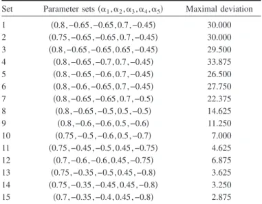
This study applied an enumeration method by sequentially adjusting the five parameter values to pretest the fitness of the spatial distribution of households’ residential location choices be-tween the model results and collected data. The modulation of each parameter value is assumed to be either +0.05 or −0.05. Following these pretests, 15 sets of values are selected for param-eters ␣1,␣2,␣3, ␣4, and␣5to show fitness consequences.
Ac-cording to the parameter calibration procedures in Phase 4 of the simulation program, the fitness is represented by the residential location with the maximal calibration deviation among all resi-dential locations in the study area. Lower maximal calibration deviation indicates better fitness consequences. The right column of Table 4 summarizes 15 sets of parameter values. The minimal deviation among all 15 sets is 2.875, and occurs in the 15th set, as shown in Table 4. The study area is represented by a two-dimensional coordinate system, and residential locations are com-posed of 120⫻150=18,000 equal-sized grids. However, average real estate prices per pyng, listed in Table 3, are categorized based on administrative districts. This study establishes a mapping layer between administrative districts and grids to convert collected data from the administrative district base into the grid base. The results of calibrated values for parameters␣1,␣2, ␣3, ␣4, and␣5
are 0.7, −0.35, −0.4, 0.45, and −0.8 as described previously. The calibrated parameters in Eq. 共13兲 represent the interactive and nonlinear effects of decision variables on the commuters’ residen-tial utility. The calibrated results show that commuter’s residenresiden-tial utility increases as total leisure time and the residual of disposal income deducted the rent and the commuting cost increase, while
it decreases as round-trip commuting time, round-trip commuting cost and the number of households at the residential location increase.
Residential Location Choices
Figs. 4共a–d兲 illustrate the surfaces of simulated numbers of house-hold at all residential locations in four time intervals, respectively. The center of CBD in this study is located at coordinate共40, 95兲. Figs. 4共a–d兲 reveal that household densities increase with decreas-ing distance from the residential locations to the CBD, resultdecreas-ing in several peaks around the CBD. When the rail transit system is fully completed in time interval four, another peak emerges at the intersection of the Nehu, Nankang, and Mucha Lines. According to Figs. 4共a–d兲, the variation of residential densities is highly sensitive to the configuration of transit networks and the location of each station. As for individual transit lines, locations with sig-nificantly higher residential densities can be found to include lo-cations at the south of both the Mingte Station 共Tamshui Line兲 and the B1 Station 共Nehu Line兲, locations at the north of the Panchiao Station共Panchiao Line兲, locations between the Chungho Line and the Mucha Line, and locations around the intersection of the Nehu, Nankang, and Mucha Lines. Comparing Figs. 4共a–d兲 with Figs. 3共a and b兲 reveals that residential densities become higher at residential sites with less commuting times and commut-ing costs. This comparison also indicates that the pattern of resi-dential density coincides with the pattern of equitravel cost contours and equitravel time contours. This phenomenon reflects that the commuting time and the commuting cost are two of the key factors when households choose their residential locations. Consequently, this study can infer the following. The closer to the CBD implies a higher household density. In addition, the higher the rent implies less commuting time and lower cost. These infer-ences correspond to the conventional location theory.
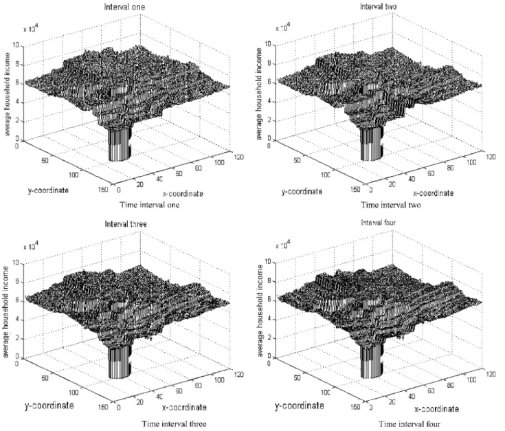
Fig. 5 illustrates average household income at each residential location in four time intervals. Fig. 5 shows that households with higher income levels prefer to reside in districts of Taipei City such as Shih-Lin, Ta-Tung, Shan, Sung-Shan, Chung-Jeng, Ta-An, Shin-Yi, and Mu-Cha in time interval one. However, there is an increased attraction of households in cities of Taipei County such as Pan-Chiao, Chung-Ho, Yong-Her, and Hsin-Tien in the succeeding time intervals due to the completion of rail transit networks in these cities. Spatial distributions of average household incomes in four time intervals are not significantly different from each other. This phenomenon implies that different income level households reveal steady preferences for their favor-ite residential locations. However, spatial variations of average household income over the study area are slightly moderated when rail transit networks are totally completed.
Conclusions and Suggestions
According to study results, impacts of rail transit networks on households’ mode choices and residential location choices are summarized as follows. First, commuters with longer travel dis-tances between homes and CBD tend to use rail transit lines as their main commuting modes, while commuters with shorter travel distances tend to use car directly to the CBD via surface streets. Second, variations in the residential densities are highly related to the configuration of transit networks and the location of each station. Finally, there are increased attractions of households in cities of Taipei County such as Pan-Chiao, Chung-Ho, Yong-Table 4. Maximal Deviation of Parameter Alternatives for␣1, ␣2, ␣3,
␣4, and␣5
Set Parameter sets共␣1,␣2,␣3,␣4,␣5兲 Maximal deviation 1 共0.8,−0.65,−0.65,0.7,−0.45兲 30.000 2 共0.75,−0.65,−0.65,0.7,−0.45兲 30.000 3 共0.8,−0.65,−0.65,0.65,−0.45兲 29.500 4 共0.8,−0.65,−0.7,0.7,−0.45兲 33.875 5 共0.8,−0.65,−0.6,0.7,−0.45兲 26.500 6 共0.8,−0.6,−0.65,0.7,−0.45兲 27.750 7 共0.8,−0.65,−0.65,0.7,−0.5兲 22.375 8 共0.8,−0.65,−0.5,0.5,−0.5兲 14.625 9 共0.8,−0.6,−0.6,0.5,−0.6兲 11.250 10 共0.75,−0.5,−0.6,0.5,−0.7兲 7.000 11 共0.75,−0.45,−0.5,0.45,−0.75兲 4.625 12 共0.7,−0.6,−0.6,0.45,−0.75兲 6.875 13 共0.75,−0.35,−0.5,0.45,−0.8兲 3.625 14 共0.75,−0.35,−0.45,0.45,−0.8兲 3.250 15 共0.7,−0.35,−0.4,0.45,−0.8兲 2.875
Her, and Hsin-Tien in the succeeding time intervals for the sake of increased mobility due to the completion of rail transit net-works. Regarding the application, the models herein can be ap-plied to highly concentrated urban areas with rail transit system that are in the planning stage or under construction. The formu-lation procedures in the commuters’ modes and route choice models as well as the households’ residential choice model, dem-onstrate the synthesis of two models in a sequential fashion. The developed models are useful for estimating travel demand for each rail transit line from a long-term planning perspective, and also for analyzing households’ spatial distribution based on sev-eral major factors. However, as data for future periods are un-available, the effectiveness of the model of commuters’ modes and route choices models and household’s residential location choice model is unclear. Future studies may justify the effective-ness of the results when further data become available in the future.
The models proposed herein have some limitations. First, the supply of land is assumed to be given and is not related to rent. Second, this study did not explicitly consider the situation of di-agonal roads in specific areas that greatly reduce travel time, since the study area is represented as a grid network and the Manhattan distance is applied to simplify the complexity of problem. Future
studies should consider diagonal roads and evaluate the benefits of diagonal roads. Third, this study is restricted to the monocen-tric city configuration and two kinds of transportation system. Results in this study can only describe the residential distribution for commuters working in the CBD of the Taipei metropolitan area and traveling by car and rail transit. To apply this model for more practical purposes, future studies with similar methods should be extended to the multicentric city configuration with all feasible transportation systems. Fourth, households’ attributes, such as working hours, hourly salary, and required residential area, are almost certainly not independent but rather are signifi-cantly and positively correlated. However, these attributes are pri-marily quantitative factors for representing individual household’s characteristics. Future studies should incorporate such correla-tions and consider qualitative factors such as individual prefer-ence and location amenity to estimate households’ residential location choices. This study formulated an optimization model rather than a choice model; therefore, the model implies that it has accounted for all factors in the residential choice of individual household. In reality, households’ residential choices might be better described as an individual probabilistic model. Fifth, the assumption of constant travel speed and fuel costs over time is unrealistic as fuel costs are dependent on travel speed, which in
Fig. 4. Households’ residential distribution
turn is affected by traffic flows in the real world. To establish a direct connection between travel time/travel cost and link flows, future studies should apply actual networks and incorporate the flow-dependent travel time function on surface streets to explore households’ mode, route, and residential location choices. Sixth, the set of explanatory variables for residential location is certainly limited, and the alphas in the residential utility function may change over time. Future studies could further consider con-straints such as two-career households, and factors such as school systems, and crime and aesthetic amenities and clustering of af-finity groups. Further, future studies could contribute by calibrat-ing the alphas for multiple years for which data are available, and could analyze any changes in weights given the various factors in the utility function.
Acknowledgments
The writers would like to thank the National Science Council of the Republic of China for financially supporting this research under Contract No. NSC 91-2415-H-009-004.
References
Alonso, W.共1964兲. Location and land use—Toward a general theory of land rent, Harvard University Press, Cambridge, Mass.
Alonso, W.共1972兲. “A theory of the urban land market.” Readings in urban economics, M. Edel and J. Rothenberg, eds., Macmillan, New York.
Bakker, A., and Creedy, J. 共2000兲. “Macroeconomic variables and in-come distribution-conditional modeling with the generalised expone-netial.” Journal of Income Distribution, 9共2兲, 183–197.
Ching, S., and Fu, F.共2003兲. “Contestability of the urban land market: An event study of Hong Kong land auctions.” Regional Science and Urban Economics, 33共6兲, 695–720.
Department of Budget, Accounting and Statistics.共1997兲. The statistical abstract of Taipei city, Taipei City Government, Taipei, R.O.C. DGBAS.共1995兲. “The report on the time utilization survey, Taiwan area,
the Republic of China.” Executive Yuan, Taipei, R.O.C.
Eliasson, J., and Mattsson, L. G.共2000兲. “A model for integrated analysis of household location and travel choices.” Transp. Res., Part A: Policy Pract., 34共5兲, 375–394.
Feng, C. M., and Yang, J. I.共1989兲. “The impact of Taipei metropolitan rail rapid red line on the regional development.” Journal of
Transpor-Fig. 5. Average household income distribution
tation Planning, 18共3兲, 349–368 共in Chinese兲.
Higano, Y.共1991兲. “Numerical analysis of urban residential location, con-sumption, and time allocation.” Papers in Regional Science: The Journal of the RSAI, 70共4兲, 439–459.
Higano, Y., and Orishimo, I.共1990兲. “Impact of spatially separated work places on urban residential location, consumption and time alloca-tion.” Papers of the Regional Science Association, 68共1兲, 9–21. Hsu, C. I., and Guo, S. P. 共2001兲. “Household-mode choice and
residential-rent distribution in a metropolitan area with surface road and rail transit networks.” Environment and Planning A, 33共9兲, 1547–1575.
Hunt, J. D., Abraham, J. E., and Weidner, T. J.共2004兲. “Household allo-cation module of Oregon2 model.” Transportation Research Record 1898, Transportation Research Board, Washington, D.C., 98–107. Hunt, J. D., and Simmonds, D. C.共1993兲. “Theory and application of an
integrated land-use and transport modeling framework.” Environ. Plann. B, 20共2兲, 221–244.
Lan, L. W. 共1980兲. The study on the fare design of the public transit system, Department of Rapid Transit Systems, Taipei City Govern-ment, Taipei, R.O.C.
Law, M. A., and Kelton, W. D.共1982兲. Simulation modeling and analysis, McGraw-Hill, New York.
Lund, J. R., and Mokhtarian, P. L. 共1993兲. “Telecommuting and resi-dential location: Theory and implications for commute travel in monocentric metropolis.” Transportation Research Record 1463, Transportation Research Board, Washington, D.C., 10–14.
Martinez, F. J.共1992兲. “The bid-choice land-use model: An integrated economic framework.” Environment and Planning A, 24共6兲, 871–885.
Newell, G. F.共1980兲. Traffic flow on transportation network, MIT Press, Cambridge, Mass.
Shibusawa, H.共1997兲. “Commuting behavior in the closed city with tele-commuting and office work.” The 36th Annual Meeting of Western Regional Science Association, Hawaii.
Shibusawa, H., and Higano, Y.共1995兲. “External economies of telecom-muting in a closed information-oriented city.” The 14th PRSCO Conf., Taipei, R.O.C.
Vaughan, R.共1987兲. Urban spatial traffic patterns, Pion, London. Waddell, P.共1993兲. “Exogenous workplace choice in residential location
models: Is the assumption valid?” Geogr. Anal., 25共1兲, 65–82. Watterson, W. T.共1993兲. “Linked simulation of land use and
transporta-tion systems: Developments and experience in the Puget Sound re-gion.” Transp. Res., Part A: Policy Pract., 27共3兲, 193–206. Wong, S. C., Zhou, C. W., Lo, H. K., and Yang, H.共2004兲. “Improved
solution algorithm for multicommodity continuous distribution and assignment model.” J. Urban Plann. Dev., 130共1兲, 14–23.
Yang, H., Yagar, S., and Iida, Y. 共1994兲. “Traffic assignment in a con-gested discrete/continuous transportation system.” Transp. Res., Part B: Methodol., 28共2兲, 161–174.
Yuan, B. H.共2003兲. “The land policy implementation for equalization of land rights: Adjustment of land value.” Thesis, Master of Political Science, National Chung Cheng Univ., Chiai, R.O.C.共in Chinese兲.