台灣二尖瓣膜脫垂病人與正常族群心率變異性之性別與姿勢差異

國

立

交

通

大

學

分子醫學與生物工程研究所

碩

士

論

文

台灣二尖瓣膜脫垂病人與正常族群心率變異性

之性別與姿勢差異

Gender Differences and Posture change of Heart Rate

Variability between Taiwanese Symptomatic Mitral Valve

Prolapse Syndrome and Normal

研 究 生：陳雅筑

指導教授：楊騰芳 教授

台灣二尖瓣膜脫垂病人與正常族群心率變異性之性別與姿勢差異

Gender Differences and Posture change of Heart Rate Variability between Taiwanese Symptomatic Mitral Valve Prolapse Syndrome and Normal

研 究 生：陳雅筑 Student：Ya-Chu Chen, RN BSc

指導教授：楊騰芳 Advisor：Ten-Fang Yang, MD MSc PhD

國 立 交 通 大 學

分 子 醫 學 與 生 物 工 程 研 究 所

碩 士 論 文

Submitted to Institute of Molecular Medicine and Bioengineering

College of Biological Science and Technology

National Chiao Tung University

in partial Fulfillment of the Requirements

for the Degree of

Master

in

Molecular Medicine and Bioengineering December 2013

Hsinchu, Taiwan, Republic of China

台灣二尖瓣膜脫垂病人與正常族群心率變異性之性別與姿勢差異

學生：陳雅筑 指導教授：楊騰芳博士

國立交通大學分子醫學與生物工程學系碩士班

摘 要

心率變異性(Heart rate variability, HRV)分析是一種測量連續心跳中， 心搏與心搏之間變化程度的方法。過去二十年間對於自主神經系統(autonomic nervous system, ANS)和心血管疾病致死率的關係性有顯著增長的認識，包括心 因性的猝死。HRV 的研究對於預測心肌梗塞、心臟瓣膜疾病、或是先天性心臟病 的病人之長期存活率是有用的，HRV 的降低是危險因子，能預測致死與心律不整 的併發。短時 HRV 能作為急性心肌梗塞預後的最初檢視。在標準的心電圖 (electrocardiogram, ECG)中，兩個 R 波波峰之間稱為 R-R 間隔(R-R interval)， 由連續的 R-R 間隔所構成的連續間距則定稱為 N-N 間隔(N-N interval)，心率變 異性就是測量 N-N 間隔的變異性。正常的心跳會因為受到自主神經系統的調控而 產生波動，因此當變異消失或明顯降低時，會產生沒有波動而完全規律的心率， 這種心率被認為是心臟自主神經調節系統異常的表現。HRV 的目的在於測量心率 快慢差異的規律，提供非侵入性的方式來測量自主神經系統的平衡性。本研究的 目地是評估在台灣二尖瓣膜脫垂的病人及正常族群中，性別與姿勢的差異是否影 響 HRV 數值。 參與實驗的二尖瓣膜脫垂病人總數 118 人，其中含 7 位男性及 111 位女性， 在 2008 年十一月至 2013 年一月期間，於台北醫學大學附屬醫院經超音波診斷確

診為二尖瓣膜脫垂之病人；另有 148 名交通大學學生及新竹地區居民，其中含 54 位男性及 94 位女性，經過 12 導程心電圖檢查及確定無其他疾病者參加實驗， 所有參加者皆為自願參與且簽下實驗同意書。本實驗所使用的機器為台灣達楷生 醫科技所研發的 DailyCare BioMedical‟s ReadMyHeart® ，使用單導程 ECG (設定 於第二導程)來做訊號的收集及分析，之後以人工編輯方式來檢查所收集到之訊 號是否出現 R 波上的錯誤。實驗過程中，受測者需變化躺姿、坐姿、站姿三種 姿勢以測量 HRV，而每一種 HRV 測量前受測者皆須休息五分鐘。所有的實驗皆 於白天時間(早上九點至下午四點)進行，以避免日夜差異對自主神經系統造成影 響。於時域分析上採用 SDNN、RMSSD 及 NN50 三項數值，頻域分析採用 TP、 LF、HF 及 LF/HF 比值。 由實驗可得知，二尖瓣膜脫垂病人與正常人相比，於時域分析中只有 SDNN 在三種姿勢中都具有統計上的差異，且此結果與頻域分析中的 TP 差異情況相 符。頻域分析中，除了躺姿測量不具有差異外，其餘姿勢的數值全部都顯示了病 人與正常人在自主神經調控上的差異。在時域分析中，無論是二尖瓣膜脫垂病人 還是正常人，男女之間在躺姿測量的 RMSSD 和 NN50 具有顯著差異。頻域分析 中，除了與 SDNN 相符的 TP 以外，其餘在各姿勢測量中都具有男女差異，顯示 男性與女性在自主神經調控上的不同。而各姿勢之間的差異，在正常族群中的時 域分析都顯示姿勢上具有差異，除了坐姿和躺姿相比時僅 RMSSD 具有統計上差 異。頻域分析也都具有意義，除了坐姿和躺姿相比時 TP 不具有顯著差異。而在 頻域統計方面，全部都顯示具有姿勢上的差異，除了在坐姿和站姿的比較中，時 域分析的 SDNN 和頻域分析的 TP 都不具有姿勢改變造成的顯著差異。從結果來 看，我們可以得知 SDNN 數值相當於 TP，此結果與往昔發表的著作相符合。正 常台灣人在性別上的 HRV 差異此前也由我們實驗室做過發表，此實驗更加一步 推論在二尖瓣膜脫垂的病人測量 HRV 也應做性別的區分。未來我們應更多收集 二尖瓣膜脫垂的男性病人以求完整這份研究。儘管時域分析或許不適合用來評估

二尖瓣膜脫垂病人的狀況，但頻域分析佐以姿勢變化的測量或許在評估二尖瓣膜 脫垂的風險上將會是有效的工具。

Gender Differences and Posture change of Heart Rate Variability between Taiwanese Symptomatic Mitral Valve Prolapse Syndrome and Normal.

Student: Ya-Chu Chen

, RN BSc

Institute of molecular medicine and bioengineering National Chiao Tung University

Abstract

Heart rate variability (HRV) is the temporal variation between sequences of

consecutive heartbeats. On a standard electrocardiogram (ECG), the duration between

two adjacent R wave peaks is termed the R-R interval. The resulting period between

adjacent QRS complexes resulting from sinus node depolarization is termed the N-N

(normal-normal) interval, and HRV is the measurement of the variability of the N-N

intervals. The last two decades have witnessed the recognition of a significant

relationship between the autonomic nervous system and cardiovascular mortality,

including sudden cardiac death. HRV investigation has its use in the prediction of

long-term survival in patients who had suffered from congestive myocardial infarction,

or had valvular or congenital heart disease. Depressed HRV is a predictor of mortality

assessed from short-term recordings may be used for initial screening of all survivors

of an acute myocardial infarction. The purpose is to evaluate the gender and postural

effects in HRV parameters between symptomatic MVPS patients and an apparently

healthy population.

A total of 118 patients, 7 males and 111 females, who had been echocardiographically

diagnosed as having MVPS at Taipei Medical University Hospital cardiology clinic

from November 2008 to January 2013, and 148 healthy people (54 males and 94

females) with normal 12-lead ECG without previous history of medical disease from

National Chiao-Tung University and residents in Hsinchu were recruited for the study.

All subjects had sign an informed consent and agree to take part in the research.

A locally developed Taiwanese machine (DailyCare BioMedical‟sReadMyHeart® )

was used to record the HRV. One lead ECG (modified lead Ⅱ) was used for signals

collection and analysis. The QRS complexes were detected and labelled automatically.

The results of the automatic analysis were reviewed subsequently, and any errors in

R-wave detection and QRS labelled were then edited manually. The subjects were

asked to rest 5 minutes before each HRV recording (Lying, sitting and standing.) All

VI

the diurnal influence of the autonomic difference.

For time-domain HRV measures, the mean N-N intervals and the standard deviation

of N-N intervals during 5 minutes (SDNN) were then calculated. For

frequency-domain HRV parameters analysis, spectral power was quantified by fast

Fourier transformation and autoregressive method for the following frequency bands:

0.15-0.4 Hz (high frequency), 0.04-0.15 Hz (low frequency). Time domain parameters

used were SDNN, RMSSD and NN50. Frequency domain parameters selected were

TP, LF, HF and LF/HF. These parameters were defined in accordance with the 1996

ACC/AHA/ESC consensus. To make sure our data is normal distribution,

Kolmogorov–Smirnov test was used at first. And then Paired Student t test was used

to characterize differences in HRV variables. All HRV variables were expressed as

mean ± SD. All statistical analyses were performed using Microsoft Excel 2007. A P

value <0.05 was determined as statistically significant.

In Time domain only SDNN between MVPS and Normal was statistically

significantly different in all positions, and so as Frequency domain‟s Total Power. In

Frequency domain all Parameters were shown to have significant differences except

differences of RMSSD and NN50 at lying both in MVPS and Normal. In frequency

domain, all parameters were statistically significantly different in all postures both in

MVPS and normal except total power. For postural changes, in normal group that

time domain parameters only RMSSD was statistically differences between lying and

sitting, but in other postural compared, all parameters were significantly different.

And it is the same as in frequency domain parameters, only TP in lying compared

with sitting posture had no difference. In MVPS group, the result of time domain

parameters and frequency domain were the same as in normal group, except in sitting

compared with standing posture. SDNN of time domain, and TP of frequency domain

had no significant difference.

From the results, we concluded that the SDNN is compatible with Total Power as

demonstrated in the previous reports. Gender specific HRV variation had been

reported in our previous study in normal Taiwanese. It is further strengthened the

digenetic criteria for HRV should be gender specific in MVPS as well. Moreover,

more male MVPS cases should be recruited for further clarification of this issue.

Although time domain parameters might not be of use for the evaluation MVPS,

frequency domain with postural changes might be a useful tool in MVPS diagnosis

VIII 誌謝 感謝楊騰芳老師在這短短的碩士班求學期間給予的指導，不僅是論文上的批 閱與學問上的教學，更讓學生有機會參加世界性的學術研討會以拓展眼界，以及 培養學生對研究實事求是的態度。於此著實獲益良多，獻上對老師最衷心的感謝 與祝福。求學期間老師多次因病入院，在此也由衷期盼老師身體康健。 口試委員王雲銘老師及曲在雯老師在百忙中撥冗替學生進行口試，並給予意 見及指導，使學生論文能更趨完備，在此也表達對兩位老師的謝意。 感謝這段求學期間生科院的老師們的授課與教導，也感謝實驗室的曾俊凱醫 師在實驗進行期間所給予的幫助，以及給予我關於畢業後志向的建議。在這段期 間，老師的助理 Isis 從日常聯絡到實驗的協助也給予我非常多的幫忙，找來許 多受測者來參加 HRV 的測量、幫忙聯絡修課學生以及處理學校行政事務，感謝她 得不吝協助。 朋友們及家人也給了我很多的鼓勵，在我遭遇瓶頸時也會給予勸導，不讓我 因為鑽牛角尖而浪費無謂的精力和時間。感謝父母讓我在求學期間給予生活上和 經濟上的協助，讓我得以無後顧之憂的完成學業。期望年事漸長的父母及家中長 輩也都能一切健康平安。

Contents Page Chapter 1 Introduction………...1 1.1 Background……..…………...………..…………...…..1 1.2 Research Propose……….………..………...….3 1.2.1 Normal Range..………..3 1.2.2 Gender Difference………..………...5 1.2.3 Postural Changes………..……….7

1.2.4 Mitral Valve Prolapse Syndrome and Normals…………..………...7

1.2.5 Age………...…...8 1.3 Overview……….…...9 Chapter 2 Electrocardiology……….…………10 2.1 Synopsis of Electrocardiology………...……..10 2.2 History of Electrocardiology…………....………..……..12 2.3 Physiology of Heart………..…20

2.4 Conduction System of Heart………....22

Chapter 3 Hear Rate Variability………...…….30

3.1 Background………..30

3.2 The history of HRV……….31

3.3 Autonomic Nervous System and HRV relationships………...33

3.3.1 Sympathetic nervous system………34

3.3.2 Parasympathetic nervous system……….35

3.3.3 Neurotransmitters and pharmacology………..36

3.4 Methods and measurements of heart rate variability parameters…37 3.4.1 Time domain methods……….38

3.4.1.1 Statistical methods………..39

3.4.1.2 Geometrical methods………..42

3.4.2 Frequency domain methods………45

3.4.3 Time-frequency signal analysis methods………51

3.5 Clinical applications of HRV………..52

3.5.1 HRV and autonomic diabetic neuropathy………...53

3.5.2 HRV and post myocardial infarction………..54

3.5.3 HRV and sudden cardiac death………...….……..54

3.5.4 HRV and chronic heart failure………...…….…55

Chapter 4 Mitral Valve Prolapse Syndrome………..…….….56

4.2 Diagnosis………....…57

4.3 Mitral Valve Prolapse Syndrome………...61

Chapter 5 Materials and Methods………...63

5.1 Materials………..63 5.2 Methods of HRV Recording………...65 5.3 Analysis of HRV………67 5.4 Statistical Analysis……….71 Chapter 6 Results………72 6.1 Normal and MVPS………..75 6.2 Gender difference………....78 6.3 Postural changes………...82

6.3.1 Postural changes in normal………...82

6.3.2 Postural changes in MVPS………...85

6.4 Results………..88

Chapter 7 Conclusions and Discussions………...……90

Reference………...96

Table Contents

Page Table 2.1 wave and intervals..………..…….….……25 Table 3.1 Selected time domain measures of HRV………..…..……42 Table 3.2 Selected frequency domain measures of HRV………..….…50 Table 3.3 Approximate correspondence of time domain and frequency domain

methods applied to 24-h ECG recordings…….…….………….……..51 Table 5.1 Age and Gender distribution with mean and standard deviation (SD)...63 Table 5.2 Time domain parameters……….69 Table 5.3 Frequency domain parameters………70 Table 5.4 Time domain parameters approximate frequency domain parameters...71 Table 6.1 Time domain HRV Parameters between Symptomatic MVP and

Normal Group………...……….76 Table 6.2 Frequency domain HRV Parameters between Symptomatic MVP and

Normal Group………...77 Table 6.3 Time domain HRV Parameters between Symptomatic MVP male and

female in all positions…….……….………...78 Table 6.4 Frequency domain HRV Parameters between Symptomatic MVP Male

and female in all positions………79 Table 6.5 Time domain HRV Parameters between normal male and female in

all positions……….80 Table 6.6 Frequency domain HRV Parameters between normal male and female

in all positions……….………81 Table 6.7 Time domain HRV Parameters between lying and sitting position in

normal group……….……….82 Table 6.8 Frequency domain HRV Parameters between lying and sitting position

in normal group……..………..83 Table 6.9 Time domain HRV Parameters between lying and standing position in

normal group……….………..83 Table 6.10 Frequency domain HRV Parameters between lying and standing position

in normal group……….……….84 Table 6.11 Time domain HRV Parameters between sitting and sitting position in

Table 6.12 Frequency domain HRV Parameters between sitting and sitting position in normal group……….………85 Table 6.13 Time domain HRV Parameters between lying and sitting position

in Symptomatic MVP group……….………85 Table 6.14 Frequency domain HRV Parameters between lying and sitting position

in Symptomatic MVP group……….………86 Table 6.15 Time domain HRV Parameters between lying and standing position

in Symptomatic MVP group……….……….86 Table 6.16 Frequency domain HRV Parameters between lying and standing position

in Symptomatic MVP group……….……….87 Table 6.17 Time domain HRV Parameters between sitting and sitting position

in Symptomatic MVP group……….……….…...87 Table 6.18 Frequency domain HRV Parameters between sitting and sitting position

Figure Contents

Page

Figure 2.1 The developing of Cardiogram...….…….………...12

Figure 2.2 The first human electrocardiogram recorded by Waller………...…….13

Figure 2.3 Definition of the deflections of the electrocardiogram…………..……14

Figure 2.4 Einthoven‟sTriangle………...…..16

Figure 2.5 Picture of Wilson central terminal and image space……….……...…17

Figure 2.6 Blood flow diagram of the human heart………...21

Figure 2.7 conduction system of heart……….24

Figure 3.1 The distribution of sympathetic nerves and parasympathetic nerves in cardiac muscle………..….37

Figure 3.2 Definitions of normal ECG waves……….39

Figure 3.3 Short-term HRV frequency domain methods………46

Figure 3.4 Consecutive sinus beat HRV intervals from a healthy subject and it associated with wavelet transform plot……….52

Figure 4.1 Classic Mitral-Valve Prolapse during Systole………...59

Figure 4.2 Classic Mitral-Valve Prolapse with Leaflet Thickening (Arrows) during Diastole……….60

Figure 5.1 The machine that we use in this study………...64

Figure 5.2 Steps of the HRV experiment………65

Figure 5.3 Steps of data analysis……….68

Figure 6.1 The ECG signal cutting for 5 minutes………...73

Figure 6.2 Time domain analysis………74

Chapter 1 Introduction

1.1 Background

Heart rate variability (HRV) is a physiological phenomenon of temporal variation

between sequences of consecutive heartbeats. On a standard electrocardiogram (ECG),

the duration between two adjacent R wave peaks is termed the R-R interval. The

resulting period between adjacent QRS complexes resulting from normal sinus node

depolarization is termed the N-N (normal-normal) interval, and HRV is the

measurement of the variability of the N-N intervals.

It has witnessed the recognition of a significant relationship between the autonomic

nervous system and cardiovascular mortality, including sudden cardiac death [1].

HRV investigation has its use in the prediction of long-term survival in patients who

had suffered from congestive heart failure, myocardial infarction, valvular or

congenital heart disease. Depressed HRV is a predictor of mortality and arrhythmic

complications independent of other recognized risk factors. HRV assessed from

myocardial infarction. Short Term (5-15 min) HRV can provide non-invasive

information on the autonomic nervous system(ANS), and was reported to be

remarkably similar to 24 hour-HRV in post-MI patients and can provide predictive

information for ventricular arrhythmias and sudden cardiac death (SCD).

Physiological and pathological process may influence N-N interval variability[24].

Under normal conditions, the balance between sympathetic and parasympathetic

activity favours the latter. Physiological influences may modulate central and

peripheral receptor activity and hence the autonomic nervous activities.

In normal subjects, a variable heart rate is the normal physiological state. It has been

suggested that the healthy heart has a long range „memory‟ which prevents it from developing extremes of pace, and that this facility erodes as age or disease

develops[5]. A loss of variability is associated with an increased mortality in patients

post myocardial infarction[4]. Drug therapy may alter HRV; beta-blocker therapy has

been shown to have a favorable effect on HRV[6][7] in patients with heart failure.

However, changes in heart rate dynamics observed before ventricular tachyarrythmias

(VTAs) in patients taking anti-arrhythmic drugs were independent of the drug

regimen[8]. And postural change influence on the HRV parameters of normal

1.2 Research Propose

A normal range of HRV in the healthy asymptomatic population has still not been

identified[2]. Without a normal range, changes in HRV are difficult to interpret and

use in evaluating disease adjustments.

The purpose is to evaluate the gender and postural effects in HRV parameters

between symptomatic Mitral Valve Prolapse Syndrome (MVPS) patients and an

apparently healthy population.

1.2.1 Normal Range

If a set of amplitudes is obtained from a group of apparently healthy individuals

within a well-defined age range, there will be a spread of measurements obtained with

a predominance of values in the middle of the group and a smaller number at either

side. In a classical situation, where there is an even spread of measurements around a

central value with the distribution, there is said to be a normal distribution[27].

who have an amplitude of a certain value[27]. When the distribution is symmetrical,

the mean of the values will be in the middle of the range. Given the set of values, it

becomes possible to calculate a mean and standard deviation (SD) for the parameter

of interest. With a classical normal distribution, the mean plus or minus twice the

standard deviation delineates approximately 95% of the range of values. Hence, if it

could be shown that a set of values possessed a normal distribution, then one method

of defining the normal range would simply be to calculate the mean and standard

deviation and proceed to derive the upper and lower limits of the normal 95 percentile

range. By taking such limits, where 2.5% of the values are excluded at either end of

the distribution, so-called outliers can be excluded.

With respect to ECG measurements, however, it was pointed out by Simonson [28]

many years ago that the range of measurements for most ECG parameters is not

normal, it tends to have a skewed distribution, for the R-wave amplitude in V5. The

longer tail of the distribution is toward the higher values with the shorter tail being

toward the lower values. To avoid this difficulty, an alternative approach for deriving

the 95 percentile limits can be adopted.

durations are referred to well-defined onsets and terminations of the component

waves[27]. In practice, the onset of the first wave in one lead does not need

necessarily coincide with the apparent onset in other leads. This leads to the concept

of introducing isoelectric segments within the QRS complex. The diagnostic

significance of these segments has not yet been evaluated, but they have a relationship

to vector orientations in a certain sense.

While the human eye at a glance may be able to say whether or not an ST segment is

concave or convex upward, it requires several measurements to establish this when

using a computer program. For this reason, Pipberger and co. [25] introduced the

concept of time normalization. It was suggested [26] that the P wave be divided into

four equal time-normalized segments. This approach has certain advantages, but it can

suffer from errors in determining the onset and termination of the components[27].

1.2.2 Gender Difference

HRV might be effect by a lot of physical factors, some like illness, age, gender, racial

or exercise. But nowadays we still do not have a HRV database all belonging to

shouldn‟t use the same HRV normal range data with other racial. We try to build the HRV normal range of Taiwanese in this research.

Gender differences in the autonomic nervous system may be present because of

developmental differences or due to the effects of prevailing levels of male and

female sex hormones[14]. Differences in the autonomic system may be due to

differences in afferent receptor stimulation, in central reflex transmission, in the

efferent nervous system and in post synaptic signaling. At each of these potential sites

of difference, there may be effects due to different size or number of neurons,

variations in receptors, differences in neurotransmitter content or metabolism as well

as functional differences in the various components of the reflex arc[14].

In human beings, resting plasma concentrations and urinary excretion of

Noradrenaline(NA) and adrenaline are generally not different between males and

females[15–17]. However, males have been found to have higher resting sympathetic

nerve activity to muscles, as determined by micro-neurography [17]. About in HRV,

the majority of studies have found women to have a lower LF/HF power ratio than

men, suggesting a preponderance of vagal over sympathetic responsiveness [18].

suggest that males have a preponderance of sympathetic over vagal control of cardiac

function compared with females. Sato and Miyake[3] found that the male subjects

were more sympathetic dominant than the female subjects. Our group has presented in

2010 ICE Lund meeting that gender difference will affect the result of HRV data[12].

1.2.3 Postural Changes

Autonomic Nervous System has a great effect in HRV. In this research we ask our

case in three postures: lying, sitting and standing. These three postures mean the

activity of sympathetic and parasympathetic nerves, and help us know how ANS work

in different situation. In normal conditions, parasympathetic nerves are more active in

lying position, and sympathetic nerves is much stimulated than parasympathetic

nerves in standing position[12].

1.2.4 Mitral Valve Prolapse Syndrome and Normals

Patients with mitral valve prolapse syndrome (MVPS) may have a variety of cardiac

and non cardiac abnormalities in addition to the characteristic valvular lesion with its

easy fatigability, abnormal cardiovascular and electrocardiographic responses to

exercise, ST- and T wave changes on resting ECGs, and a variety of atrial and

ventricular arrhythmias[10][11].

The presence of chest pain, ST-T-wave abnormalities, and arrhythmias suggests the

possibility of a functional disorder involving the autonomic nervous system[9]. Many

of the clinical features of the MVPS are found in other conditions which have been

attributed to some type of autonomic dysfunction, e.g., neuro-circulatory or

vaso-regulatory asthenia[13].

1.2.5 Age

Under the age of 50, sympathetic nerve activity was significantly greater in men than

women [22]. In the study of Kuo et al.[23], the percentage LF power was significantly

higher in the younger males than the younger females whilst the percentage HF power

was significantly higher in the younger females than the younger males. Yamasaki et

al.[18] also found a decline with age for both HF and LF power. The decline with age

Because of the data is not enough, we did not discuss about aging problem in this

study.

1.3 Overview

In this study, it includes seven part. First chapter is introduction, and then chapter 2 is

Electrocardiology. Chapter 3 is about Heart Rate Variability, and Chapter 4 is Mitral

Valve Prolapse. In chapter 5 is the method and material about this study, and chapter

Chapter 2 Electrocardiology

2.1 Synopsis of Electrocardiology

Electrocardiology in its broadest term is the study of the electric field generated by

individual cells of the heart. Electrocardiology includes Electrophysiology and

Biophysics. The most common subject is Electrocardiogram (ECG or EKG from the

German Elektrokardiogramm). Electrocardiography is a transthoracic interpretation of

the electrical activity of the heart over a period of time, as detected by electrodes

attached to the outer surface of the skin and recorded by a device external to the

body[29].

It was first proposed by Lempert in 1976[29] and just over one hundred years since

the human electrocardiogram was first recorded by a physiologist Augustus D. Waller

at the St. Mary‟s Hospital in London U.K.[32] and almost seventy years since the first

unipolar electrocardiographic lead was introduced by Frank Wilson in the University

of Michigan, U.S.A. (Wilson et al, 1934)[30]. Fisch[33] emphasized the fact that

simple to use. The electrocardiogram also provides unique information that cannot be

obtained by any other investigative technique.

With the advent of computer techniques, the electrocardiogram can be recorded and

interpreted with such equipments. So nowadays, it is more practical to use the

electrocardiogram as an aid for clinical diagnosis. ECG is used to measure the rate

and regularity of heartbeats, as well as the size and position of the chambers[29].

Nowadays, ECG becomes an important examination to aid clinical diagnosis. Some of

the early work in electrocardiography was carried out in Europe, where today there

are still considerable developmental efforts being expended, particularly in the field of

computer-assisted electrocardiograms being recorded, there is a need for their

automated analysis of ECGs. But the computer does not have the human emotional

factor and distraction in the interpretation of electrocardiograms. Therefore, it

provides the advantage of fast interpretation of ECG and significant improvement of

2.2 History of Electrocardiology

L.G. Horan[31] has divided the history of electrocardiogram into three dedicate. “Era of Electricity”, it ended in 1750. And then started an “Era of Bioelectricity”, it was from 1750 to 1900. Finally, the “Era of Cardiac Electric Sequence” is from 1900 to nowadays.

Fig. 2.1 The developing of Cardiogram[31].

The first galvanometer had been invented by the mid 19th century. Physiologists were

he was criticized by Volta who thought when different metals contact, it could

generate electric current. Volta‟s work led to the development of batteries[34].

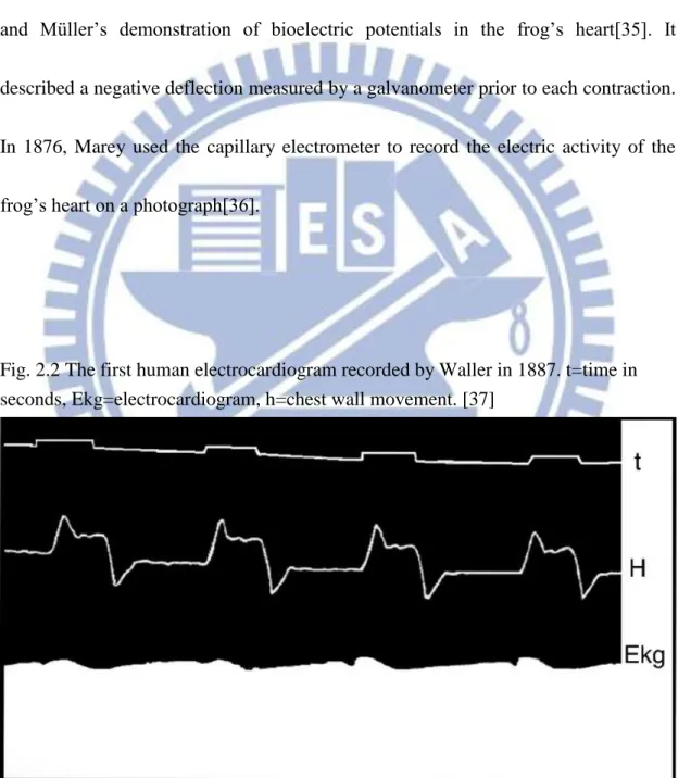
The first recording of cardiac electrical activity was performed in 1856 by Kölliker

and Müller‟s demonstration of bioelectric potentials in the frog‟s heart[35]. It described a negative deflection measured by a galvanometer prior to each contraction.

In 1876, Marey used the capillary electrometer to record the electric activity of the

frog‟s heart on a photograph[36].

Fig. 2.2 The first human electrocardiogram recorded by Waller in 1887. t=time in seconds, Ekg=electrocardiogram, h=chest wall movement. [37]

Waller investigated that recording from the limbs of animals is the same with in man.

He published his observations of the electrocardiogram recorded from his dog using

the capillary electrometer in 1889. It was stated by Willem Einthoven in 1912 that

Waller first introduced the term “electrocardiogram” into physiological science [38]. Einthoven designed a device to record cardiac electrical potentials from the surface of

the body, and he introduced the concept known as “Einthoven‟s triangle”. It means the body was represented in electrical terms by an equilateral triangle, from

which the mean QRS axis can be calculated[39]. Einthoven also used the terminology

of P, Q, R, S T to describe the deflection of the electrocardiogram (Fig 2.3) and

developed a method called “Telecardiography” in 1906 for transmitting the electrocardiogram over telephone lines[32].

Fig. 2.3 Definition of the deflections of the electrocardiogram by Einthoven[40]. S=time in 0.1 second, Lower tracing shows P, Q, R, S & T deflection of the ECG.

Einthoven[38] introduced lead I, II, and III and a variety of different

The three limb leads, denoted I, II, and III can be represented as follows:

Lead I = EL - ER

Lead II = EF - ER

Lead III = EF - EL

Where EL, ER and EF denote the potential at the left and fight arms and left leg. It

follows that:

II = I + III

Fig. 2.4 Einthoven‟sTriangle[53].

Sir Thomas Lewis had used bipolar chest leads in the studies of cardiac rhythmic

disorders[41][42]. His measurement of epicardial activation established the

hypothesis on the excitation of the myocardium.

During the 1920s, Frank Wilson undertook many studies correlating

electrocardiographic findings (essentially limb leads I, II, and III) with abnormalities

such as ventricular hypertrophy and bundle branch block. Their concept of

“Ventricular Grandient” is still used in nowadays. Wilson‟s major contribution is his “central terminal”[43], which means unipolar chest leads can be recorded.

However, the concept allows the potential variation at a single point on the chest to be

recorded with potential obtained by averaging the potentials of right and left arms and

the left leg. This record is known as a “unipolar” lead. If the potential at the Wilson central terminal is denoted by EWCT then

EWCT = 1/3 (ER + EL + EF)

Fig. 2.5 (A) picture of Wilson central terminal; (B) image space of Wilson central terminal[44].

The next stage of the unipolar lead was to specify six precordial positions for the

exploring electrodes, which were slightly different from the six leads V1-V6 used

In 1942, Goldberger introduced the “augmented unipolar limb lead” to electrocardiography. He removed the Wilson central terminal connection from the

limb on which the exploring lead was placed and this augmented the potential

recorded by 50% [46]. Mathematically, the relationship between the modified

unipolar right arm lead (modified VR), which is modified by the removal of the right

arm connection to the Wilson central terminal, and the resultant potential of the

modified Goldberger‟s Terminal (EGT) for this lead is as follow:

VR = ER - EWCT Modified VR= ER - EGT = ER - 1/2 (EL + EF) = 3/2 ER - 1/2 (EL + EF + ER) =3/2[ER -1/3 (EL + EF + ER)] =3/2 [ER - EWCT]

The modified VR became known as aVR. Similar circuitry was introduced to record

modified VL and VF, i.e. aVL and aVF.

The development of conventional 12-lead electrocardiography was then

completed. There were three limb lead: I, II, and III from Einthoven; three

augmented unipolar limb leads: aVR, aVL, and aVF from Goldberger‟s modification of Wilson‟s central terminal; and six praecordial leads V1-V6 arising out of Wilson‟s central terminal.

The development of electrocardiography continued in different ways and progressed

through the research of several gifted electrocardiographers and electrophysiologists.

The improvements in the techniques of measurement, recording, interpretation and

modeling as well as the elaboration of many theories have contributed to the widening

2.3 Physiology of heart

The human heart has a mass of between 250 and 350 grams[47]. It has four chambers,

two superior atria and two inferior ventricles. The atria are the receiving chambers

and the ventricles are the discharging chambers.

The pathways of blood through the human heart are part of the pulmonary and

systemic circuits. These pathways include the tricuspid valve, the mitral valve, the

aortic valve, and the pulmonary valve[48]. The mitral and tricuspid valves are

classified as the atrioventricular valves. The aortic and pulmonary semi-lunar valves

separate the left and right ventricle from the pulmonary artery and the aorta

respectively. The interatrioventricular septum separates the left atrium and ventricle

from the right atrium and ventricle, dividing the heart into two functionally separate

Fig. 2.6 Blood flow diagram of the human heart[49].

Blood flows through the heart in one direction, from the atria to the ventricles, and out

of the great arteries. Blood is prevented from flowing backwards by the tricuspid,

bicuspid, aortic, and pulmonary valves.

The function of the right heart is to collect de-oxygenated blood, in the right atrium,

from the body (via superior and inferior vena cavae) and pump it, via the right

ventricle, into the lungs (pulmonary circulation) so that carbon dioxide can be

dropped off and oxygen picked up. The left side collects oxygenated blood from the

lungs into the left atrium. From the left atrium the blood moves to the left ventricle

which pumps it out to the body (via the aorta). On both sides, ventricles are thicker

the wall surrounding the right ventricle due to the higher force needed to pump the

blood through the systemic circulation. Starting in the right atrium, the blood flows

through the tricuspid valve to the right ventricle. It is pumped out of the pulmonary

semilunar valve and travels through the pulmonary artery to the lungs. From there,

blood flows back through the pulmonary vein to the left atrium. It then travels through

the mitral valve to the left ventricle, from where it is pumped through the aortic

semilunar valve to the aorta and to the rest of the body. The deoxygenated blood

finally returns to the heart.

2.4 Conduction System of Heart

The normal electrical conduction in the heart allows the impulse that is generated by

the sinoatrial node (SA node) be propagated to and stimulate the myocardium. It is the

ordered stimulation of the myocardium that allows efficient contraction of the heart.

In order to maximize the efficiency of contraction and cardiac output, the conduction

a) Substantial atrial to ventricular delay. It allows the atria to completely empty their

contents into the ventricles. The atria connected only via the AV node which briefly

delays the signal.

b) Coordinated contraction of ventricular cells. The ventricles must maximize systolic

pressure to force blood through the circulation.

c) Absence of tetany. After contracting the heart must relax to fill up again.

Signals arising in the SA node stimulate the atria to contract and travel to the AV

node. After a delay, the stimulus is conducted through the bundle of His to the

Purkinje fibers and the endocardium at the apex of the heart, and then finally to the

ventricular epicardium[50].

The heart is a functional syncytium. In a functional syncytium, electrical impulses

propagate freely between cells in every direction, so that the myocardium functions as

a single contractile unit. This property allows rapid, synchronous depolarization of the

potentially allows the propagation of incorrect electrical signals. These gap junctions

can close to isolate damaged or dying tissue, as in a myocardial infarction.

Fig. 2.7 conduction system of heart[22].

A typical ECG tracing of the cardiac cycle consists of a P wave, a QRS complex, a T

Table 2.1 wave and intervals. [52]

description

RR interval The interval between an R wave and the next R wave: Normal resting heart rate is between 60 and 100 bpm.

P wave During normal atrial depolarization, the main electrical vector is directed from the SA node towards the AV node, and spreads from the right atrium to the left atrium. This turns into the P wave on the ECG.

PR interval The PR interval is measured from the beginning of the P wave to the beginning of the QRS complex. The PR interval reflects the time the electrical impulse takes to travel from the sinus node through the AV node and entering the ventricles. The PR interval is, therefore, a good estimate of AV node function.

J-point The point at which the QRS complex finishes and the ST segment begins, it is used to measure the degree of ST elevation or depression present.

ST segment The ST segment connects the QRS complex and the T wave. The ST segment represents the period when the ventricles are depolarized. It is isoelectric.

T wave The T wave represents the repolarization (or recovery) of the ventricles. The interval from the beginning of the QRS complex to the apex of the T wave is referred to as the absolute refractory period. The last half of the T wave is referred to as the relative refractory period (or vulnerable period).

ST interval The ST interval is measured from the J point to the end of the T wave.

QT interval The QT interval is measured from the beginning of the QRS complex to the end of the T wave. A prolonged QT interval is a risk factor for ventricular tachyarrhythmias and sudden death. It varies with heart rate and for clinical relevance requires a correction for this, giving the QTc.

U wave The U wave is hypothesized to be caused by the repolarization of the interventricular septum. They normally have low amplitude, and even more often completely absent. They always follow the T wave and also follow the same direction in amplitude. If they are too prominent, suspect hypokalemia, hypercalcemia or hyperthyroidism usually[24].

In normal conditions, electrical activity is generated by the SA node. This electrical

impulse is propagated throughout the right atrium, and through Bachmann's bundle to

the left atrium, stimulating the myocardium of the atria to contract. The conduction of

the electrical impulse throughout the atria is seen on the ECG as the P wave. As the

electrical activity is spreading throughout the atria, it travels via specialized pathways,

known as internodal tracts, from the SA node to the AV node.

The AV node functions as a critical delay in the conduction system. Without this

delay, the atria and ventricles would contract at the same time, and blood wouldn't

flow effectively from the atria to the ventricles. The delay in the AV node forms much

of the PR segment on the ECG. And part of atrial repolarization can be represented by

PR segment.

The distal portion of the AV node is known as the Bundle of His. The Bundle of His

splits into two branches in the interventricular septum, the left bundle branch and the

right bundle branch. The left bundle branch activates the left ventricle, while the right

bundle branch activates the right ventricle. The left bundle branch is short, splitting

into the left anterior fascicle and the left posterior fascicle. The left posterior fascicle

to ischemic damage. The left posterior fascicle transmits impulses to the papillary

muscles, leading to mitral valve closure. As the left posterior fascicle is shorter and

broader than the right, impulses reach the papillary muscles just prior to

depolarization, and therefore contraction, of the left ventricle myocardium. This

allows pre-tensioning of the chordae tendinae, increasing the resistance to flow

through the mitral valve during left ventricular contraction. This mechanism works in

the same manner as pre-tensioning of car seatbelts.

The two bundle branches taper out to produce numerous Purkinje fibers, which

stimulate individual groups of myocardial cells to contract. The spread of electrical

activity through the ventricular myocardium produces the QRS complex on the ECG.

The last event of the cycle is the repolarization of the ventricles. It is the restoring of

the resting state. In the ECG, repolarization includes the J wave, ST-segment, and T-

and U-waves[51].

Cardiac muscle is a syncytium, and the heart is composed of two syncytiums: the

atrial syncytium that constitutes the walls of the two atria, and the ventricular

from the ventricles by fibrous tissue that surrounds the atrioventricular (A-V) valvular

openings. Potentials are conducted only by way of a specialized conductive system:

A-V bundle. This division of the muscle of the heart into two functional syncytiums

allows the atria to contract a short time ahead of ventricular contraction, which is

important for effectiveness of heart pumping. The action potential recorded in a

ventricular muscle fiber, averages about 105 millivolts. The intracellular potential

rises from a very negative value, about -85 millivolts, between beats to a slightly

positive value, about +20 millivolts, during each beat. After the initial spike, the

membrane remains depolarized for about 0.2 second, exhibiting a plateau, followed at

the end of the plateau by abrupt repolarization.

In cardiac muscle, the action potential is caused by two types of channels[50]: (a) the

fast sodium channels as the same in skeletal muscle and (b) another entirely different

population of slow calcium channels, which are also called calcium-sodium channels.

During this time, a large quantity of both calcium and sodium ions flows through

these channels to the interior of the cardiac muscle fiber, and this maintains a

prolonged period of depolarization, causing the plateau in the action potential. Further,

process, while the calcium ions that cause skeletal muscle contraction are derived

Chapter 3 Hear Rate Variability

3.1 Background

Heart rate variability (HRV) is the temporal variation between sequences of

consecutive heartbeats. On a standard electrocardiogram (ECG), the maximum

upwards deflection of a normal QRS complex is at the peak of the R wave, and the

duration between two adjacent R wave peaks is termed the R-R interval. The ECG

signal requires editing before HRV analysis can be performed, a process requiring the

removal of all non-sinus-node-originating beats. The resulting period between

adjacent QRS complexes resulting from sinus node depolarization is termed the N-N

(normal-normal) interval[1], and HRV is the measurement of the variability of the

N-N intervals. The last two decades have witnessed the recognition of a significant

relationship between the autonomic nervous system and cardiovascular mortality,

including sudden cardiac death[1]. HRV investigation as its use in the prediction of

long-term survival in patients who has suffered from congenital myocardial infarction,

or had valvular or congestive heart disease. Depressed HRV is a predictor of mortality

assessed from short-term recordings may be used for initial screening of all survivors

of an acute myocardial infarction.

In 1996, the European Society of Cardiology and the North American Society of

Pacing and Electrophysiology to constitute a Task Force charged with the

responsibility of developing appropriate standards. The goals of the Task Force were

to: standardize nomenclature and develop definitions of terms; specify standard

methods of measurement; define physiological and pathophysiological correlates;

describe currently appropriate clinical applications, and identify areas for future

research. „Heart Rate Variability‟ has become the conventionally accepted term to describe variations of both instantaneous heart rate and RR intervals[1].

3.2 The history of HRV

The clinical relevance of heart rate variability(HRV) was first appreciated in 1965

when Hon and Lee[54] noted that fetal distress was accompanied by changes in

beat-to-beat variation of the fetal heart, even before there was a detectable change in

the rate. In the 1970s, Sayers and others[77] focused attention on the existence of

used short-term HRV (15 min) measurements as a maker of diabetic autonomic

neuropathy[55]. In 1977, Wolf et al.[56] showed that patients with reduced HRV after

a myocardial infarction had an increased mortality, and this was confirmed by studies

showing that HRV is an accurate predictor of mortality post myocardial infarction

(MI)[57-59]. In 1981, Akselrod et al. introduced power spectral analysis of heart rate

fluctuations to quantitatively evaluate beat-to-beat cardiovascular control[60]. The clinical importance of HRV became apparent in the late 1980s when it was confirmed

that HRV was a strong and independent predictor of mortality following an acute

myocardial infarction[57-59].

HRV has also been investigated as a tool to predict the risk of sudden cardiac

death(SCD)[61], and Low HRV is an independent risk factor for the development of

later cardiac arrest in survivors of cardiac arrest[61]. Both reduced HF power and

reduced LF power are independent predictors of later sudden death following survival

from cardiac arrest[61]. Reduction in HF power appears superior at risk-stratifying

3.3 Autonomic Nervous System and HRV relationships

HRV is affected by Autonomic nervous system. The ANS is part of the peripheral

nervous system, it affects heart rate, digestion, respiratory rate, salivation, perspiration,

pupillary dilation, urination, and sexual arousal[63].

The ANS included: sympathetic nervous system and the parasympathetic nervous

system, which operate independently in some functions and interact co-operatively in

others. In many cases they activate opponent where one activates a physiological

response and the other inhibits it. The sympathetic division begins at the thoracic and

lumbar (T1-L2/3) portions of the spinal cord. The parasympathetic division begins at

the cranial nerves (CN 3, CN7, CN 9, CN10) and sacral (S2-S4) spinal cord. The

sympathetic division typically functions in actions requiring quick responses. The

parasympathetic division functions with actions that do not require immediate

reaction. These two systems should be seen as permanently modulating vital

3.3.1 Sympathetic nervous system

The sympathetic nervous system controls most of the body's internal organs. As in the

flight-or-fight response, stress is thought to counteract the parasympathetic system,

which generally works to promote maintenance of the body at rest. The functions of

both the parasympathetic and sympathetic nervous systems are not so

straightforward[64][65].

There are two kinds of neurons involved in the transmission through the sympathetic

system: pre-ganglionic and post-ganglionic. The shorter preganglionic neurons

originate from the thoracolumbar region of the spinal cord and travel to a ganglion,

often one of the paravertebral ganglia, where they synapse with a postganglionic

neuron. The long postganglionic neurons extend across most of the body from

there[66]. At the synapses within the ganglia, preganglionic neurons release

acetylcholine. In response to the stimulus, postganglionic neurons release

norepinephrine[67].

The sympathetic nervous system is responsible for many homeostatic mechanisms in

stress response commonly known as the fight-or-flight response. This response is also

known as sympatho-adrenal response of the body, as the preganglionic sympathetic

fibers that end in the adrenal medulla secrete acetylcholine (Ach) which activates the

great secretion of epinephrine and to a lesser extent norepinephrine from it. Therefore,

this response acts primarily on the cardiovascular system is mediated directly via

impulses transmitted through the sympathetic nervous system and indirectly via

catecholamines secreted from the adrenal medulla[78].

3.3.2 Parasympathetic nervous system

The parasympathetic system is responsible for stimulation of "rest-and-digest" or

"feed and breed" activities that occur when the body is at rest, especially after eating,

including sexual arousal, salivation, lacrimation, urination, digestion and defecation.

Sympathetic and parasympathetic divisions typically function in opposition to each

other. This natural opposition is better understood as complementary in nature rather

than antagonistic. The sympathetic division typically functions in actions requiring

quick responses; whereas the parasympathetic division functions with actions that do

The afferent fibers of the autonomic nervous system are not divided into

parasympathetic and sympathetic fibers as the efferent fibers are[68]. Instead,

autonomic sensory information is conducted by general visceral afferent fibers.

The parasympathetic nervous system uses chiefly ACh as its neurotransmitter,

although some peptides (such as cholecystokinin) may act on the parasympathetic

nervous system as a neurotransmitter[69][70]. Most transmissions occur in two stages:

When stimulated, the preganglionic nerve releases ACh at the ganglion, which acts on

nicotinic receptors of postganglionic neurons. The postganglionic nerve then releases

ACh to stimulate the muscarinic receptors of the target organ.

3.3.3 Neurotransmitters and pharmacology

Sympathetic ganglionic neurons release norepinephrine at the effector organs and act

on adrenergic receptors, with the exception of the sweat glands and the adrenal

medulla: Acetylcholine is the preganglionic neurotransmitter for both divisions of the

ANS, as well as the postganglionic neurotransmitter of parasympathetic neurons.

Nerves that release acetylcholine are said to be cholinergic. In the parasympathetic

muscarinic receptors. At the adrenal medulla, there is no postsynaptic neuron. The

presynaptic neuron releases acetylcholine to act on nicotinic receptors. Stimulation of

the adrenal medulla releases epinephrine into the bloodstream, producing a

widespread increase in sympathetic activity.

Fig. 3.1 The distribution of sympathetic nerves and parasympathetic nerves in cardiac muscle[79].

3.4 Methods and measurements of heart rate variability parameters

Variations in heart rate may be evaluated by a number of methods. The most widely

methods, and nonlinear methods.

3.4.1 Time domain methods

R is a point corresponding to the peak of the QRS complex of the ECG wave; and

R-R interval is all intervals between adjacent QRS complexes resulting from sinus

node depolarizations. The term "N-N interval" is used in place of R-R interval to

emphasize the fact that the processed beats are "normal" beats[1].

Simple time domain variables that can be calculated include the mean NN interval,

the mean heart rate, the difference between the longest and shortest NN interval, the

difference between night and day heart rate, etc. Other time domain measurements

that can be used are variations in instantaneous heart rate secondary to respiration, tilt,

Fig. 3.2 Definitions of normal ECG waves[76].

3.4.1.1 Statistical methods

From a series of instantaneous heart rates or cycle intervals, more complex statistical

time-domain measures can be calculated. These may be divided into two classes:

(a) those derived from direct measurements of the NN intervals or instantaneous heart

rate.

Those variables may be derived from analysis of the total electrocardiographic

recording or may be calculated using smaller segments of the recording period. All

these measurements of short-term variation estimate high frequency variations in

heart rate and thus are highly correlated.

SDNN(standard deviation of all normal to normal intervals) is the simplest variable to

calculate. Since variance is mathematically equal to total power of spectral analysis,

SDNN reflects all the cyclic components responsible for variability in the period of recording. The total variance of HRV increases with the length of analyzed

recording[71].

SDANN(standard deviation of average normal to normal intervals) calculated over

short periods, usually 5 min, which is an estimate of the changes in heart rate due to

cycles longer than 5 min.

SDNN index (standard deviation of all normal to normal intervals index) is the mean

of the 5-min standard deviation of the NN interval calculated over 24 h, which

RMSSD (The square root of the mean of the sum of the squares of differences

between adjacent NN intervals), the square root of the mean squared diVerences of

successive NN intervals.

NN50 (Number of pairs of adjacent NN intervals differing by more than 50 ms in the

entire recording), the number of interval differences of successive NN intervals

greater than 50 ms.

pNN50 (NN50 count divided by the total number of all NN intervals), the proportion

Table 3.1 Selected time domain measures of HRV[1].

Variable Units Description

SDNN ms Standard deviation of all NN intervals.

SDANN ms Standard deviation of the averages of NN intervals in all 5 min segments of the entire recording.

RMSSD ms The square root of the mean of the sum of the squares of differences between adjacent NN intervals.

SDNN index ms Mean of the standard deviations of all NN intervals for all 5 min segments of the entire recording.

SDSD ms Standard deviation of differences between adjacent NN

intervals.

NN50 count Number of pairs of adjacent NN intervals differing by more than 50 ms in the entire recording. Three variants are possible counting all such NN intervals pairs or only pairs in which the first or the second interval is longer.

pNN50 % NN50 count divided by the total number of all NN intervals.

3.4.1.2 Geometrical methods

The NN intervals can also be converted into a geometric pattern[1], as the sample

density distribution of NN interval durations, sample density distribution of

differences between adjacent NN intervals, Lorenz plot of NN or RR intervals, etc.

detected and the NN interval variation[1]. The triangular HRV index considers the

major peak of the histogram as a triangle with its baseline width corresponding to the

amount of NN interval variability, its height corresponds to the most frequently

observed duration of NN intervals. The triangular HRV index is an estimate of the

overall HRV[1].

Three general approaches are used in geometric methods:

(a) a basic measurement of the geometric pattern (e.g. the width of the distribution

histogram at the specified level) is converted into the measure of HRV.

(b) the geometric pattern is interpolated by a mathematically defined shape (e.g. approximation of the distribution histogram by a triangle, or approximation of the

differential histogram by an exponential curve) and then the parameters of this

mathematical shape are used.

(c) the geometric shape is classified into several pattern-based categories which represent different classes of HRV (e.g. elliptic, linear and triangular shapes of Lorenz

Geometrical methods are less affected by the quality of the recorded data; however,

the recording time should be at least 20 minutes[1], which means that short-term

recordings cannot be assessed by geometric methods.

The HRV triangular index measurement is the integral of the density distribution (i.e.

the number of all NN intervals) divided by the maximum of the density distribution.

Using a measurement of NN intervals on a discrete scale, the measure is

approximated by the value:

HRV triangular index= (total number of NN intervals) / (number of NN intervals in

the modal bin)

And that is dependent on the length of the bin, i.e. on the precision of the discrete

scale of measurement.

The triangular interpolation of NN interval histogram (TINN) is the baseline width of

the distribution measured as a base of a triangle, approximating the NN interval

distribution (the minimum square difference is used to find such a triangle). Both

the lower than by the higher frequencies[59]. Other geometric methods are still in the

phase of exploration and explanation.

The major advantage of geometric methods lies in their relative insensitivity to the

analytical quality of the series of NN intervals[72].

The major disadvantage is the need for a reasonable number of NN intervals to

construct the geometric pattern. Recordings of at least 20 minutes and preferably 24

hours should be used to ensure the correct performance of the geometric methods.

3.4.2 Frequency domain methods

Several methods are available[74] since the late 1960s. Power spectral density (PSD),

using parametric or nonparametric methods, provides basic information on the power

distribution across frequencies. Methods for the calculation of PSD may be generally

classified as nonparametric and parametric. In most instances, both methods provide

comparable results. The advantages of the nonparametric methods are: (a) the

simplicity of the algorithm employed (Fast Fourier Transform (FFT) in most of the

are smoother spectral components that can be distinguished independent of

preselected frequency bands, easy postprocessing of the spectrum with an automatic

calculation of low-frequency and high-frequency power components with an easy

identification of the central frequency of each component. Beside FFT,

Auto-Regressiv (AR) model is another choice. These two kinds of models have

different figures, but the consequences could be compared.

Fig. 3.3 Short-term HRV frequency domain methods.

In short-term recordings three main spectral components are distinguished in a

spectrum calculated from the recordings: very low frequency(VLF), low frequency

(LF), and high frequency (HF) components. Measurement of VLF, LF and HF power

also be measured in normalized units (n.u.) which represent the relative value of each

power component in proportion to the total power minus the VLF component. LF

norm= LF/(Total Power–VLF) x 100, and HF norm= HF/(Total Power–VLF) x 100.

The representation of LF and HF in n.u. emphasizes the controlled and balanced

behavior of the two branches of the autonomic nervous system. Beside, normalization

tends to minimize the effect on the values of LF and HF components of the changes in

total power. Although HRV assessed from short-term recordings provides prognostic

information, HRV measured in nominal 24-h recordings is a stronger risk

predictor[1].

Long-term recordings Spectral analysis may also be used to analyze the sequence of

NN intervals in the entire 24-h period. The result then includes an ultra-low frequency

component (ULF), VLF, LF and HF components. The slope of the 24-h spectrum can

also be assessed on a log–log scale by linear fitting the spectral values[1].

Because of the differences in the interpretation of the results, the spectral analyses of

short-term and long-term electrocardiograms should always be distinguished.

Frequency domain methods would be preferred to the time domain methods when

recordings should not be substantially extended. Thus, recording of approximately 1

min is needed to assess the HF components of HRV while approximately 2 min are

needed to address the LF component. In order to standardize short-term HRV, 5 min

recordings of a stationary system are preferred[1].

Short-term recordings do have several advantages. First, they are quick to perform

and to analyze. Second, short-term recordings can be made under controlled

conditions to ensure standardization. Third, they can be made under a variety of

conditions such as different postural, psychological or pharmacologic interventions.

But in long-term recordings, physiological mechanisms of heart period modulations

responsible for LF and HF power components cannot be considered stationary during

the 24-h period[75]. But spectral analysis performed in the 24-h period as well as

spectral results from shorter segments (e.g. 5 min) averaged over the entire 24-h

period provide averages of the modulations attributable to the LF and HF

components[1].

Vagal activity is the major contributor to the HF component, and disagreement exists

in respect of the LF component[1][54]. When LF expressed in normalized units, it is a

and vagal activity. Consequently, the LF/HF ratio is considered by some investigators

to mirror sympatho/vagal balance or to reflect sympathetic modulations. Physiological

interpretation of lower frequency components of HRV (VLF and ULF components)

warrants further elucidation. It is important to note that HRV measures fluctuations in