受限緊砂回填土對擋土牆主動土壓力之影響

(1)

國立交通大學

土木工程學系碩士班

碩士論文

受限緊砂回填土對擋土牆主動土壓力之影響

Active Earth Pressure on Retaining Walls

with Constrained Dense Backfill

研究生 : 黃亭淵

指導教授 : 方永壽博士

(2)

受限緊砂回填土對擋土牆主動土壓力之影響

Active Earth Pressure on Retaining Walls

with Constrained Dense Backfill

研究生: 黃亭淵

Student：Ting-Yuan Huang

指導教授：方永壽博士

Advisor：Dr. Yung-Show Fang

國立交通大學土木工程學系碩士班

碩士論文

A Thesis

Submitted to the Department of Civil Engineering

College of Engineering

National Chiao Tung University

in Partial Fulfillment of the Requirements

for the Degree of

Master of Engineering

in Civil Engineering

September, 2010

Hsinchu, Taiwan, Republic of China

中華民國一百年九月

(3)

受限緊砂回填土對擋土牆主動土壓力之影響

研究生 : 黃亭淵指導教授 : 方永壽博士

國立交通大學土木工程學系碩士班

摘要

本論文以試驗方法探討作用於垂直剛性擋土牆的側向土壓力，此擋土牆逐漸遠離受限之緊砂回填土。模型擋土牆設備試驗以渥太華砂為回填土材料，回填土高0.5 公尺，岩石介面與水平線夾角 β 為 0°，60°，70°，80 °和90°。本研究使用震動夯實法製做緊砂回填土，以一座鋼製傾斜界面板模擬束制背填土的岩石介面。試驗結果顯示，震動夯實造成的額外水平應力隨擋土牆主動位移而消散。隨著逐漸減小的水平距離 b，和逐漸增大的介面板傾斜角度 β，介面板逐漸侵入主動土楔，造成位於接近擋土牆底部的側向土壓力減少。於不同的 b 與 β 值，試驗獲得的主動土壓合力比 Coulomb 解大 25.1%至比 Coulomb 解小 24.2%。主動土壓合力作用點位置隨 β 角的增加而上升。於不同的 b 與 β 值，試驗得到的主動土壓合力作用點(h/H)a 值分布為 0.475 至 0.333。無因次化的主動土壓力矩介於 0.0801 至 0.0599 之間，大於Coulomb 主動土壓力矩 33.5%至 0%。鄰近傾斜岩石介面的存在略為降低檔土牆抗傾倒之安全係數，依據 Coulomb 主動土壓力理論預估求出之抗傾倒安全係數將不安全。關鍵字：主動土壓力、受限背填土、土壓力、模型試驗、擋土牆、緊砂

(4)

Active Earth Pressure on Retaining Walls

with Constrained Dense Backfill

Student : Ting-Yuan Huang Advisor : Dr. Yung-Show Fang Department of Civil Engineering

National Chiao Tung University

Abstract

This paper presents the experimental data of lateral earth pressure acting on a vertical rigid wall, which moved away from a limited backfill of dry sand. A model retaining-wall facility was used and dense Ottawa sand was used as backfill material. The thickness of backfill was 500 mm and rock face inclination angles of 0, 60, 70, 80 and 90 degrees were investigated. The dense backfill was prepared by vibratory compaction method. To simulate an inclined rock face, a steel interface plate was used. Test results showed that the extra lateral earth pressure due to vibratory compaction dissipated with the active wall movement. As the interface angle β increased or spacing b decreased, the inclined rock face intruded the active soil wedge, the earth pressure decreased near the base of the wall. The experimental active soil thrustfor different b and β varied from 25.1% greater to 24.2% less than Coulomb’s solution. The point of application of the active soil thrust ascended with increasing β angle. For tests with different b and β, the experimental (h/H)a varied from 0.475 to 0.333. The experimental normalized driving moment varied from 0.0801 to 0.0599, which was about 33.5% to 0% greater than Coulomb’s theoretical solution. The existence of a nearby inclined rock face would slightly decrease the factor of safety against overturning. The estimation of the factor of safety against overturning with Coulomb’s theory would be unsafe.

Keywords: Active pressure; Constrained backfill; Earth pressure; Model test; Retaining wall; Dense Sand

(5)

Acknowledgements

The author wishes to give his sincere appreciation to his advisor, Dr. Yung-Show Fang for his continuous encouragement, helpful discussions and enthusiastic suggestions in the past two years. The author also wants to express his appreciation to the members of his supervisory committee, Dr. Yi-Wen Pan, Dr. Jhih-Jhong Liao, Dr. An-Bin Huang, Dr. Shen-Yu Shan and Dr. Chih-Ping Lin for their teaching and valuable suggestions. In addition, the author also thanks Mr. Ming-Yi Huang and Mr. Kuan-Yu Chen for their suggestions and discussions.

Appreciation is extended to all my friends and classmates, especially for Mr. Yu-An Huang, Mr. Cheng Liu, Mr. Jia-Hao Dai, Mr. Yi-Chang Li and Mr. Cheng-You Li for their support and encouragement.

Finally, the author would dedicate this thesis to his parents for their continuing encouragement and moral support.

(6)

List of Tables

Table 2.1. Comparison of experimental and theoretical values………...53 Table 3.1. Technical Information of the Eccentric Motor………54 Table 6.1 Test Program……….55

(10)

List of Figures

Fig. 1.1. Retaining walls with constrained backfill 56

Fig. 1.2. Model test for b = 2000 mm 57

Fig. 1.3. Model test for b = 0 58

Fig. 2.1. Coulomb’s theory of active earth pressure 65

Fig. 2.2. Coulomb’s active pressure determination 66

Fig. 2.3. Rankine’s theory of active earth pressure 66

Fig. 2.4. Failure surface in soil by Terzaghi’s log-spiral method 67 Fig. 2.5. Evaluation of active earth pressure by trial wedge method 68

Fig. 2.6 Stability of soil mass abd1f1 69

Fig. 2.7. Active earth pressure determination with Terzaghi’s log-sprial failure surfaces

70 Fig. 2.8. Fascia retaining wall of backfill width B and wall friction F 71

Fig. 2.9. Horizontal element of backfill material 72

Fig. 2.10. Distribution of soil pressure against fascia walls due to partial support from wall friction F

73 Fig. 2.11. University of Manchester model retaining wall 74

Fig. 2.12. Earth pressure with wall movement 75

Fig. 2.13. Failure surfaces 76

Fig. 2.14. Distributions of horizontal earth pressure at different wall displacement 77 Fig. 2.15. Change of normalized lateral pressure with translation wall displacement 78 Fig. 2.16. Coefficient of horizontal active thrust as a function of soil density 79

(11)

Fig. 2.17. Model wall test with b = 100 mm and β = 50° 80 Fig. 2.18. Distribution of horizontal earth pressure for b = 0 and various β angles 81 Fig. 2.19. Distribution of horizontal earth pressure for b = 50 mm and various β

angles

82 Fig. 2.20. Distribution of horizontal earth pressure for b = 100 mm and various β

angles

83 Fig. 2.21. Variation of Kh and h/H with wall movement for b = 0 84 Fig. 2.22. NCTU model retaining wall with interface plate supports 85 Fig. 2.23. Distribution of active earth pressure at different interface inclination angle

for b = 150, 250, 350 and 500 mm

86 Fig. 2.24. Variation of earth pressure coefficient Kh with wall movement for b = 150,

250, 350 and 500 mm

87 Fig. 2.25. Variation of total thrust location with wall movement for b = 150, 250, 350

and 500 mm

88

Fig. 2.26. Typical geometry: (a) analyzed (b) notation 89

Fig. 2.27. Predictions by ReSSA versus centrifugal test results for φ = 36° and m = ∞

90

Fig. 2.28. Analysis results 90

Fig. 2.29. Typical geometry of backfill zone behind a retaining wall used in this study 91 Fig. 2.30. The finite element mesh for a retaining wall with limited backfill space

(β=70° and b=0.5m)

91 Fig. 2.31. Distribution of earth pressures with the depth at various wall displacements

for walls in translation (T mode)

92 Fig. 2.32. Variation of the coefficient of active earth pressures

(Ka(Computed)/Ka(Coulomb)) with the inclination of rock faces at various fill widths (b) for walls undergoing translation

93

Fig. 2.33. Variation of the location of resultant (h/H) of active earth pressures with the inclination of rock faces at various fill widths (b) for walls undergoing translation (T mode)

(12)

Fig. 2.34. Definition of plane strain state-of-stress 94

Fig.3.1. NCTU Model Retaining-Wall Facility 95

Fig.3.2. NCTU model retaining wall 96

Fig.3.3. Displacement transducer (Kyowa DT-20D) 96

Fig. 3.4. Locations of pressure transducers on NCTU model wall 97 Fig.3.5. Locations of pressure transducers on model wall 98

Fig. 3.6. Soil pressure transducer (Kyowa PGM-0.2KG) 98

Fig. 3.7. Data acquisition system 99

Fig. 3.8. Side-View of Square Vibratory Compactor 100

Fig. 3.9. Square Vibratory Soil Compactor 101

Fig. 3.10. 500 mm × 90 mm vibratory strip compactor 102

Fig. 3.11. Strip vibratory compactor 103

Fig. 3.12. Top and bottom of Strip vibratory soil compactor 104 Fig. 4.1. NCTU model retaining wall with inclined interface plate 105

Fig. 4.2. Steel interface plate 106

Fig. 4.3. Steel interface plate 107

Fig. 4.4. NCTU model retaining wall system with interface plate and supports 108

Fig. 4.5 Soil bin with base support block 109

Fig. 4.6. Top supporting beam 110

Fig. 4.7. Steel interface plate and top supporting beam 111

Fig. 4.8. Dimensions of base supporting block 112

Fig. 4.9. Base supporting block 113

Fig. 4.10. Base supporting boards 114

Fig. 5.1. Grain size distribution of Ottawa sand 115

Fig. 5.2. Shear box of direct shear test device 116

Fig. 5.3. Relationship between unit weight γ and internal friction angle φ 117 Fig. 5.4. Direct shear test to determinate wall friction 118 Fig. 5.5. Relationship between unit weight γ and wall friction angle δw 119 Fig. 5.6. Plastic-sheet lubrication layers on side walls 120

(13)

Fig. 5.7. Schematic diagram of sliding block test 121

Fig. 5.8 Sliding block test apparatus 122

Fig. 5.9 Variation of side-wall friction angle with normal stress 123 Fig. 5.10. Direct shear test to determine interface friction angle 124 Fig. 5.11. Relationship between unit weight γ and interface plate friction angle δi 125 Fig. 5.12. Variation of friction angles φ, δi, δw, δsw with soil unit weight γ 126 Fig. 5.13. Relationship between relative density of soil and drop height 127

Fig. 5.14. Soil hopper 128

Fig. 5.15. Raining of sand from soil hopper 129

Fig. 5.16. Compaction Procedure with Square Soil Compactor (Top-View) 130 Fig. 5.17. Compaction Procedure with Strip Soil Compactor (Top-View) 130

Fig. 5.18. Strip Soil Compactor with Wood spacer 131

Fig. 5.19. Soil-density control cup 132

Fig. 5.20. Soil-density cup 133

Fig. 5.21 (a). Locations of density cups for b = 350 mm and β = 90° 134

Fig. 5.22 Distribution of relative density 136

Fig. 6.1. Model wall test without adjacent interface plate (b = 2,000 mm) 137 Fig. 6.2. Model wall test without adjacent interface plate for layer 1 (b = 2,000 mm) 139 Fig. 6.3. Model wall test without interface plate (b = 2,000 mm) 140 Fig. 6.4. Distribution of horizontal earth pressure for b = 2,000 mm (Test 0427-1) 141 Fig. 6.5. Distribution of horizontal earth pressure for b = 2,000 mm (Test 0511-1) 141 Fig. 6.6. Earth pressure coefficient Kh versus wall movement for b = 2,000 mm 142 Fig. 6.7. Location of total thrust application for b = 2,000 mm 142 Fig. 6.8. Model wall test with interface inclination = 60° and b = 0 143 Fig. 6.9. Distribution of horizontal earth pressure for b = 0 and = 60° (Test

0820-1)

145 Fig. 6.10. Distribution of horizontal earth pressure for b = 0 and = 60°(Test

0820-2)

145 Fig. 6.11. Model wall test with interface inclination = 70° and b = 0 146

(14)

Fig. 6.12. Distribution of horizontal earth pressure for b = 0 and = 70° (Test 0820-3)

0825-1)

148 Fig. 6.14. Model wall test with interface inclination = 80° and b = 0 149 Fig. 6.15. Distribution of horizontal earth pressure for b = 0 and = 80° (Test

0825-2)

0825-3)

151 Fig. 6.17. Earth pressure coefficient Kh versus wall movement for b = 0 and =

60°

70°

80°

153 Fig. 6.20. Location of total thrust application for b = 0 and = 60° 154 Fig. 6.21. Location of total thrust application for b = 0 and = 70° 154 Fig. 6.22. Location of total thrust application for b = 0 and = 80° 155 Fig. 6.23. Model wall test with interface inclination = 60° and b = 50 mm 156 Fig. 6.24. Distribution of horizontal earth pressure for b = 50 mm and = 60° (Test

0722-2)

158 Fig. 6.25. Distribution of horizontal earth pressure for b = 50 mm and = 60°(Test

0722-3)

158 Fig. 6.26. Model wall test with interface inclination = 70° and b = 50 mm 159 Fig. 6.27. Distribution of horizontal earth pressure for b = 50 mm and = 70° (Test

0723-1)

0723-3)

161 Fig. 6.29. Model wall test with interface inclination = 80° and b = 50 mm 162

(15)

Fig. 6.30. Distribution of horizontal earth pressure for b = 50 mm and = 80° (Test 0801-1)

164 Fig. 6.31. Distribution of horizontal earth pressure for b = 50 mm and = 80°(Test 0801-2)

164 Fig. 6.32. Model wall test with interface inclination = 90° and b = 50 mm 165 Fig. 6.33. Distribution of horizontal earth pressure for b = 50 mm and = 90° (Test 0730-1)

0730-2)

167 Fig. 6.35. Earth pressure coefficient Kh versus wall movement for b = 50 mm

and = 60°

and = 70°

and = 80°

and = 90°

169 Fig. 6.39. Location of total thrust application for b = 50 mm and = 60° 170 Fig. 6.40. Location of total thrust application for b = 50 mm and = 70° 170 Fig. 6.41. Location of total thrust application for b = 50 mm and = 80° 171 Fig. 6.42. Location of total thrust application for b = 50 mm and = 90° 171 Fig. 6.43. Model wall test with interface inclination = 60° and b = 100 mm 172 Fig. 6.44. Distribution of horizontal earth pressure for b = 100 mm and = 60°

(Test 0718-2)

174 Fig. 6.45. Distribution of horizontal earth pressure for b = 100 mm and =

60°(Test 0718-3)

174 Fig. 6.46. Model wall test with interface inclination = 70° and b = 100 mm 175 Fig. 6.47. Distribution of horizontal earth pressure for b = 100 mm and = 70°

(Test 0716-2)

(16)

Fig. 6.48. Distribution of horizontal earth pressure for b = 100 mm and = 70° (Test 0716-3)

(Test 0715-2)

180 Fig. 6.51. Distribution of horizontal earth pressure for b = 100 mm and = 80°

(Test 0715-4)

(Test 0711-1)

(Test 0714-2)

and = 60°

184 Fig. 6.56. Earth pressure coefficient Kh versus wall movement for b = 100 mm and = 70°

and = 80°

and = 90°

185 Fig. 6.59. Location of total thrust application for b = 100 mm and = 60° 186 Fig. 6.60. Location of total thrust application for b = 100 mm and = 70° 186 Fig. 6.61. Location of total thrust application for b = 100 mm and = 80° 187 Fig. 6.62. Location of total thrust application for b = 100 mm and = 90° 187 Fig. 6.63. Model wall test with interface inclination = 70° and b = 150 mm 188 Fig. 6.64. Distribution of horizontal earth pressure for b = 150 mm and = 70°

(Test 0708-1)

(Test 0708-2)

(17)

Fig. 6.66. Model wall test with interface inclination = 80° and b = 150 mm 191 Fig. 6.67. Distribution of horizontal earth pressure for b = 150 mm and = 80°

(Test 0702-1)

(Test 0702-2)

(Test 0627-2)

(Test 0628-2)

and = 70°

and = 80°

and = 90°

198 Fig. 6.75. Location of total thrust application for b = 150 mm and = 70° 199 Fig. 6.76. Location of total thrust application for b = 150 mm and = 80° 199 Fig. 6.77. Location of total thrust application for b = 150 mm and = 90° 200 Fig. 6.78. Model wall test with interface inclination = 80° and b = 250 mm 201 Fig. 6.79. Distribution of horizontal earth pressure for b = 250 mm and = 80°

(Test 0621-2)

(Test 0622-2)

(Test 0613-1)

(Test 0615-1)

(18)

Fig. 6.84. Earth pressure coefficient Kh versus wall movement for b = 250 mm and = 80°

and = 90°

207 Fig. 6.86. Location of total thrust application for b = 250 mm and = 80° 208 Fig. 6.87. Location of total thrust application for b = 250 mm and = 90° 208 Fig. 6.88. Model wall test with interface inclination = 90° and b = 350 mm 209 Fig. 6.89. Distribution of horizontal earth pressure for b = 350 mm and = 90°

(Test 0603-1)

(Test 0603-2)

and = 90°

212 Fig. 6.92. Location of total thrust application for b = 350 mm and = 90° 212 Fig. 6.93. Model wall test with interface inclination = 90° and b = 500 mm 213 Fig. 6.94. Distribution of horizontal earth pressure for b = 500 mm and = 90°

(Test 0518-1)

(Test 0530-1)

and = 90°

216 Fig. 6.97. Location of total thrust application for b = 500 mm and = 90° 216 Fig. 6.98. Distribution of active earth pressure at different interface inclination

angle for b = 0

217 Fig. 6.99. Distribution of active earth pressure at different interface inclination

angle for b = 50 mm

angle for b = 100 mm

(19)

Fig. 6.101. Distribution of active earth pressure at different interface inclination angle for b = 150 mm

220 Fig. 6.105. Variation of earth pressure coefficient Kh with wall movement for b =

0

50 mm

100 mm

150 mm

250 mm

350 mm

500 mm

224 Fig. 6.112. Variation of total thrust location with wall movement for b = 0 225 Fig. 6.113. Variation of total thrust location with wall movement for b = 50 mm 225 Fig. 6.114. Variation of total thrust location with wall movement for b = 100 mm 226 Fig. 6.115. Variation of total thrust location with wall movement for b = 150 mm 226 Fig. 6.116. Variation of total thrust location with wall movement for b = 250 mm 227

(20)

Fig. 6.118. Variation of total thrust location with wall movement for b = 500 mm 228

Fig. 6.119. Variation of Ka,h versus β angle 229

Fig. 6.120. Variation of (h/H)a versus β angle 230

Fig. 6.121. Normalized overturning momentversus β angle 231 Fig. 6.122. (a) Apparatus for investigating arching in layer of sand above yielding

trap door in horizontal platform; (b) pressure on platform and trap door before and after slight lowering of door

232 Fig. 6.123. Soil arching at two levels in cohesionless backfill 233

(21)

List of Symbols

b = Distance between Interface Plate and Model Wall Cu = Uniformity Coefficient

Dr = Relative Density

D10 = Diameter of Ottawa Sand whose Percent finer is 10% D60 = Diameter of Ottawa Sand whose Percent finer is 60% emax = Maximum Void Ratio of Soil

emin = Minimum Void Ratio of Soil F _{= Force}

Gs = Specific Gravity of Soil h = Location of Total Thrust

(h/H)a = Point of Application of Active Soil Thrust H = Effective Wall Height

i = Slop of Ground Surface behind Wall Ko = Coefficient of Earth Pressure At-Rest Ka = Coefficient of Active Earth Pressure Kh = Coefficient of Horizontal Earth Pressure

Ka,h = Coefficient of Horizontal Active Earth Pressure Pa = Total Active Force

β = Angle of Inclination Rock Face S = Wall Displacement

T = Translation

z = Depth from Surface σh = Horizontal Earth Pressure σN = Normal Stress

(22)

γ = Unit Weight of Soil

φ = Angle of Internal Friction of Soil δi = Angle of Interface Friction δsw = Angle of Side-Wall Friction

δw = Angle of Wall Friction

(23)

Chapter 1 Introduction

Traditionally, civil engineers build retaining structures to resist the active force from the backfill. In most cases, civil engineers calculate the active earth pressure behind a retaining wall using either Coulomb’s or Rankine’s theory. They postulate that earth pressure distribution is linear, and the location of resultant force is located at 1/3 of the wall hight above the wall base. If there is a rock face near the retaining wall,see Fig. 1.1. the influence of the adjacent rock face on the active earth pressure deserved to be investigated.This thesis studies the effects of a constrained dense cohesionless backfill on the active earth pressure against a retaining wall as shown

in Fig. 1.1. In the figure, an inclined rock face is near the retaining wall. The backfill

is constrained and the active soil failure wedge behind the wall can not develop fully. Under such a condition, the active earth pressure may be different from Coulomb’s and Rankine’s solutions.

1.1 Objectives of Study

Valuable studies associated with earth pressure on retaining walls with constrained backfill had been conducted. Based on the arching theory, Spangler and Handy (1984) developed a theoretical equation for calculating the lateral earth pressure acting on the wall of a silo. The granular particles in the silo were constrained by the vertical silo walls. Based on the limit equilibrium method and the computer program ReSSA 2.0, Leshchinsky et al. (2004) numerically investigated the lateral earth pressure on a Mechanically-Stabilized-Earth wall with constrained fill. Fan and Fang (2010) used the non-linear finite element program PLAXIS

(PLAXIS BV, 2002) to investigate the earth pressure against a rigid wall close to an inclined rock face. Huang (2009) used the model retaining wall facilities at National Chiao Tung University to investigate the active earth pressure on retaining walls

(24)

with loose sand backfill near an inclined rock face. Chen (2010) extended the study of Huang (2009) by setting extra position for the inclined rock face (b=150,250,350 and 500 mm). However, the test results reported by Huang (2009) and Chen (2010) were limited for a model wall with a loose backfill (relative density = 36%).

From a practical point of view, it would be necessary to know what is influence of an inclined rock face on active earth pressure for a retaining wall with compacted dense backfill. In this study, the sandy backfill was compacted with a vibratory compactor to a relative density of about 79%. The experimental results are compared with theoretical and numerical solutions.

1.2 Research Outline

To study the effects of an adjacent inclined rock face on the active earth pressure, the National Chiao Tung University (NCTU) model retaining wall facility was modified to investigate the effects of a constrained backfill on the active earth pressure. In Fig. 1.1, the major parameters considered were the horizontal spacing b between the wall and the base of the rock face, and the rock face inclination angle β.

Fig. 1.2 shows the model wall with the backfill for b = 2000 mm. Fig. 1.3 to Fig. 1.9

shows all constrained condition for backfill for b = 50, 100, 150, 250, 350, and 500 mm with β = 60°, 70°, 80°, and 90°. For all tests, the height of the backfill H was 0.5 m, and air-dry Ottawa sand was used as the backfill material. To obtain a dense backfill, the soil was compacted by a square and a strip vibratory compactor to achieve the desired relative density of 79%. The variation of lateral earth pressure σh was measured with the soil pressure transducers (SPT) on the surface of the model wall. Based on experimental results, the distribution of active earth pressure was obtained. Based on the test results, the magnitude of active soil thrust and the location of the active thrust were calculated and compared with the Coulomb and Rankine solutions.

(25)

1.3 Organization of Thesis

This paper is divided into the following parts: Chapter 1: Introduction of the subject

Chapter 2: Review of past investigations regarding the active earth pressures theories, numerical studies and laboratory test results

Chapter 3: Description of experimental apparatus

Chapter 4: Description of the Interface plate and supporting system Chapter 5: Characteristics of the backfill and interfaces

Chapter 6: Test results regarding horizontal earth pressure and active soil thrust Chapter 7: Conclusions and design recommendations

(26)

Chapter 2 Literature Review

Geotechnical engineers frequently use the Coulomb and Rankine’s earth pressure theories to calculate the active earth pressure behind retaining structures. These theories are discussed in the following sections. Mackey and Kirk (1967), Fang and Ishibashi (1986), Huang (2009) and Chen (2010) made experimental investigations regarding active earth pressure. Frydman and Keissar (1987) used the centrifuge technique to test a small model wall. Numerical investigation was studied by Leshchinsky, et al. (2004) and Fan and Fang (2009). Their major findings are introduced in this chapter.

2.1 Active Earth Pressure Theories

2.1.1 Coulomb Earth Pressure Theory

Coulomb (1776) proposed a method of analysis that determines the resultant horizontal force on a retaining system for any slope of wall, wall friction, and slope of backfill. The Coulomb theory is based on the assumption that soil shear resistance develops along the wall and the failure plane. Detailed assumptions are made as the followings:

1. The backfill is isotropic and homogeneous.

2. The rupture surface is plane, as plane BC in Fig. 2.1(a). The backfill surface AC is a plane surface as well.

3. The frictional resistance is distributed uniformly along the rupture surface BC.

(27)

5. There is a friction force between soil and wall when the failure wedge moves toward the wall.

6. Failure is a plane strain condition.

In order to develop an active state, the wall is designed to move away from the soil mass. If the wedge ABC in Fig. 2.1(a) moves down relative to the wall, the wall friction angle δ will develop at the interface between the soil and wall. Let the weight of wedge ABC be W and the force on BC be F. With the given value θ and the summation of vertical forces and horizontal forces, the resultant soil thrust P can be calculated as shown in Fig. 2.1(b).

Similarly, the active forces of other trial wedges, such as ABC2, ABC3 in Fig

2.2 can be determined. The maximum value of Pa thus determined is the Coulomb's active force. P_a H2K_a 2 1_γ = (2.1) where

Pa = total active force per unit length of wall Ka = coefficient of active earth pressure

γ _{= unit weight of soil}

H = height of wall And ₂ 2 2 ) sin( ) sin( ) sin( ) sin( 1 ) sin( sin ) ( sin ⎭ ⎬ ⎫ ⎩ ⎨ ⎧ + − − + + − + = i i K_a β δ β φ δ φ δ β β β φ (2.2) where

φ_{= internal friction angle of soil}

(28)

β_{= slope of back of the wall to horizontal}

i = slope of ground surface behind wall

2.1.2 Rankine Earth Pressure Theory

Rankine (1857) considered the soil in a state of plastic equilibrium and used essentially the same assumptions as Coulomb. The Rankine theory further assumes that there is no wall friction and failure surfaces are straight planes, and that the resultant force acts parallel to the backfill slope. Detailed assumptions are made as the followings:

1. The backfill is isotropic and homogeneous.

2. The retaining wall is a rigid body. The wall surface is vertical and the friction force between the wall and the soil is neglected.

Rankine assumed no friction between wall surface and backfill, and the backfill is cohesionless. The earth pressure on plane AB of Fig. 2.3(a) is the same as that on plane AB inside a semi-infinite soil mass in Fig. 2.3(b). For active condition, the active earth pressure σa at a given depth z can be expressed as:

σa =γzKa (2.3) The total active force Pa per unit length of the wall is equal to

P_a H2K_a

2 1_γ

= (2.4)

The direction of resultant force Pa is parallel to the ground surface as Fig. 2.3(b), where ) cos (cos cos ) cos (cos cos cos 2 2 2 2 φ φ − + − − = i i i i i Ka (2.5)

(29)

2.1.3 Terzaghi General Wedge Theory

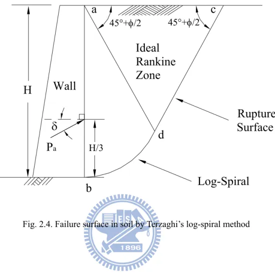
The assumption of plane failure surface made by Coulomb and Rankine, however, does not apply in practice. Terzaghi (1941) suggested that part of the failure surface in the backfill under an active condition was a log spiral curve, like the curve bd in Fig. 2.4. But the failure surface dc is still assumed a plane.

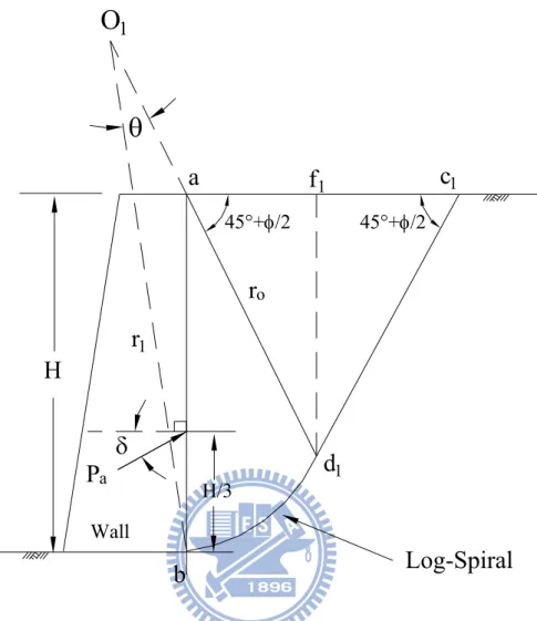
Fig. 2.5 illustrates the procedure to elevate the active resistance by trial wedge method (Terzaghi and Peck, 1967). The line d1c1 makes an angle of 45o +φ 2 with the surface of the backfill. The arc bd1 of trial wedge abd1c1 is a logarithmic spiral formulated as the following equation

θtanφ 0 1 re

r = (2.6)

O1 is the center of the log spiral curve in Fig. 2.5, where O1b = r1, O1d1 = r0, and ∠bO1d1 = θ . For the equilibrium and the stability of the soil mass abd1f1 in Fig. 2.6, the following forces per unit width of the wall are considered:

1. Soil weight per unit width in abd1f1: W1 = γ × (area of abd1f1)

2. The vertical face d1f1 is in the zone of Rankine’s active state; hence, the force

Pd1 acting on the face is

) 2 45 ( tan ) ( 2 1 2 2 1 1 φ γ °− = _d d H P (2.7) where Hd1 = d1f1

Pd1 acts horizontally at a distance of Hd1/3 measured vertically upward from d1.

(30)

3. The resultant force of the shear and normal forces dF, acting along the surface of sliding bd1. At any point of the curve, according to the property of the logarithmic spiral, a radial line makes an angle φ with the normal. Since the resultant dF makes an angle φ with the normal to the spiral at its

point of application, its line of application will coincide with a radial line and will pass through the point O1.

4. The active force per unit width of the wall P1 acts at a distance of H/3 measured vertically from the bottom of the wall. The direction of the force P1 is inclined at an angle δ with the normal drawn to the back face of the wall.

5. Moment equilibrium of W1, Pd1, dF and P1 about the point O1:

W₁

[ ]

l₂ +P_d₁

[ ]

l₃ +dF (0)= P₁

[ ]

l₁ (2.8) or

[

₁ ₂ ₁ ₃

]

1 1 1 l P l W l P = + d (2.9)

where l2, l3, and l1 is the moment arm for force W₁, P_d1, and P₁, respectively. The trial active forces per unit width in various trial wedges are shown in Fig. 2.7. Let P1, P2, P3, …, and Pn be the force that respectively correspond to the trial wedges 1, 2, 3, …, and n. The forces are plotted to the same scale as shown in the upper part of the figure. A smooth curve is plotted through the points 1, 2, 3, …, n. The maximum P3 of the smooth curve defines the active force Pa per unit width of the wall.

2.1.4 Spangler and Handy’s Theory

(31)

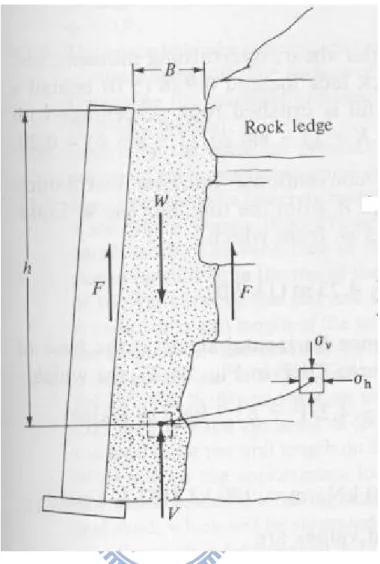
problem of fascia retaining walls. Fig. 2.8 defines the soils with a width B bounded by two unyielding frictional boundaries (the rock face and wall face). The vertical force equilibrium of the thin horizontal soil element in Fig. 2.9 requires

dh V Bdh B V K dV V + )+2 μ = +γ ( (2.10)

This is a linear differential equation, the solution for which is

( ) μ γ μ K e B V B h K 2 1 2 / 2 − − = (2.11) where

μ = tan δ, the coefficient of friction between the soil and the wall

γ = unit weight of the soil

B = backfill width h = backfill depth (i.e. z)

K = the coefficient of lateral earth pressure

V = the vertical force

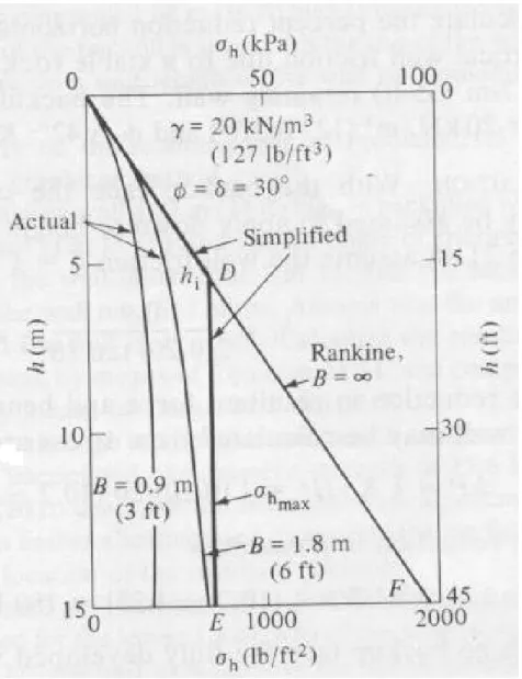
From the solution of eq.(2.11), an equation for lateral earth pressure σh can be calculated = _⎢⎣⎡ − − K ( )hB _⎥⎦⎤ h e B μ μ γ σ 2 1 2 (2.12)

Some solutions for different values of B are shown in Fig. 2.10. The soil pressure, instead of continuing to increase with increasing values of h, levels off at a maximum value σh,max defined as follows.

(32)

δ γ μ γ σ tan 2 2 max , B B h = = (2.13)

2.2 Laboratory Model Retaining Wall Tests

2.2.1 Model Study by Mackey and Kirk

Mackey and Kirk (1967) experimented on lateral earth pressure by using a steel model wall. This soil tank was made of steel with internal dimensions of 36 in. long × 16 in. wide × 15 in. high (914 mm × 406 mm × 381 mm) as shown in Fig. 2.11. In this investigation, when the wall moves away from the soil, the earth pressure decreases (see Fig. 2.12) and then increases slightly until it reaches a constant value. Mackey and Kirk reported that if the backfill is loose, the active earth pressure obtained experimentally are within 14 percent off those obtained theoretically from almost any of the methods list in Table 2.1.

Mackey and Kirk utilized a powerful beam of light to observe the failure surface in the backfill. It could trace the position of the shadow, formed by changes of the sand surface in different level. It was found that for each backfill, the failure surface in the backfill due to the translational wall movement was approximated a curve in the backfill (Fig. 2.13), rather than a plane assumed by Coulomb.

2.2.2 Model Study by Fang and Ishibashi

Fang and Ishibashi (1986) conducted laboratory model experiments to investigate the distribution of the active stresses due to three different wall movement modes: (1) rotation about top (RT mode), (2) rotation about base (RB mode), and (3) translation (T mode). The experiments were conducted at the University of Washington.

(33)

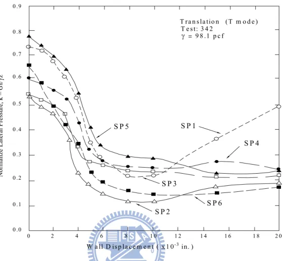
Fig. 2.14 shows the horizontal earth pressure distributions at different translational wall movements. The measured active stress is slightly higher than Coulomb's solution at the upper one-third of wall height H is 3.33 ft (1.01 m), approximately in agreement with Coulomb's prediction in the middle one-third, and lower than Coulomb' at the lower one-third of wall surface. However, the magnitude of the active total thrust Pa at S = 20 10× −3 in. (0.5 mm) is nearly the same as that calculated from Coulomb's theory.

Fig. 2.15 shows lateral earth pressures measured at various depths decreased rapidly with the translational active wall displacement. Most measurements reach the minimum value at approximately 10 10_× −3

in (0.25 mm, or 0.00025H) wall displacement and stay steady thereafter.

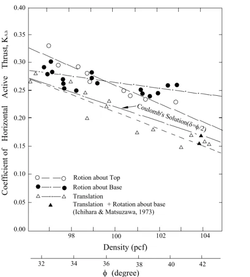
Fig. 2.16 shows the Ka as a function of soil density and internal friction angle. In this figure, the Ka value decreases with increasing φ angle. The Coulomb’s solution might underestimate the coefficient Ka for rotational wall movements.

2.2.3 Model Study by Huang

Huang (2009) used the model retaining wall facilities at National Chiao Tung University, the movable model retaining wall and its driving system are illustrated in Fig. 2.17. The model wall is a 1,000-mm-wide, 550-mm-high, and 120-mm-thick solid plate, and is made of steel. The soil bin is fabricated of steel members with inside dimensions of 2,000 mm x 1,000 mm x 1,000 mm. The effective wall-height H (or height of backfill above wall base) is only 500 mm.

To investigate the active earth pressure on retaining walls near an inclined rock face. The parameters considered for that study were the rock face inclination angles β = 0°, 50°, 60°, 70°, 80° and 90°, the horizontal spacing b = 0, 50 mm and 100 mm. In Fig. 2.17, the interface plate was inserted into the base support block at the horizontal distance of b = 100 mm from the base of the model wall, and with the

(34)

inclination angles β =50°.

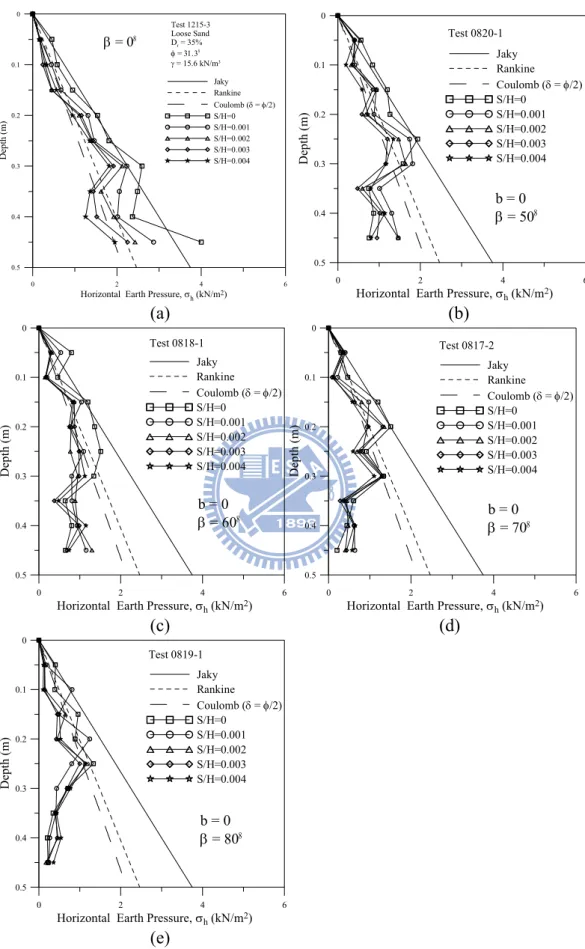
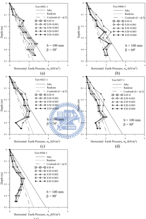
Distributions of horizontal earth pressure σh measured at different stages of horizontal wall displacements S/H was illustrated in Fig. 2.18, Fig. 2.19 and Fig. 2.20. It has been found that for the wall with a nearby inclined rock face, the active earth pressure measured at the upper part of the wall was in good agreement with Coulomb’s prediction. However, the active pressure measured at the lower part of the wall was lower than Coulomb’s prediction. If the inclined rock face was adjacent to the wall, only a thin layer of backfill was sandwiched between the rock face and the wall. It was impossible for the active soil wedge to develop behind the wall, therefore the active pressure was less than Coulomb’s prediction.

For b = 0, Fig. 2.21 (a) presents the variation of horizontal earth pressure coefficient Kh as a function of wall movement for various β angles. The magnitude of active earth pressure coefficient decreased with increasing interface inclination angle β. Fig. 2.21 (b) showed the variations of the point of application of the soil force as a function of wall movement for various β angles. It was apparent that the points of application of the active soil forces ascended with increasing β angle.

2.2.4 Model Study by Chen

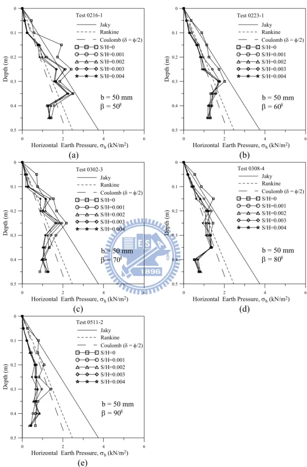
Chen (2010) extended the study of Huang (2009) by setting extra position for the inclined rock face (b=150,250,350 and 500 mm). In Fig 2.22, the interface plate was inserted into the base support block at the horizontal distance of b = 150 mm from the base of the model wall, and with the inclination angles β.

Fig. 2.23 shows the distributions of horizontal earth pressure σh measured at different stages of horizontal wall displacements S/H for various b and β. For b = 500 mm, the measured σh was close to Coulomb’s solution, the measured stress was not affected by the existence of the vertical plate. With the approahing of the interface plate, σh decreased with the increasing of angles β and the decreasing of

(35)

space b.

Variation of earth pressure coefficient Kh with wall movement illustrated in Fig. 2.24. with the approaching of the interface plate, the soil mass behind the wall decreased. The active earth pressure coefficient Ka,h decreased with increasing interface inclination angle β or decreasing spacing b.

Fig.2.25 show the variation of total thrust location with wall movement, the point of application of active soil thrust was located at about H/3 above the wall base.

2.3 Numerical Studies

2.3.1 Numerical Study by Leshchinsky et al.

Leshchinsky et al. (2004) used the limit equilibrium method with computer program ReSSA 2.0 (ADAMA, 2003) to numerically investigate the lateral earth pressure acting on a Mechanically-Stabilized-Earth wall. A baseline 5m-high wall was specified,the geometrical modeling was shown in Fig. 2.26(a). A single layer of reinforcement at 1/3 of the height of the wall was simulated in the analysis. In Fig. 2.26 the foundation was considered as competent bedrock to eliminate external effects on its stability. Various types of reinforced cohesionless fill were used in the analysis, all having a unit weight of γ = 20 kN/m3_{and the internal angle of friction φ} of the fill varying from 20° to 45°. Fig. 2.26(b) shows the base width of the fill was B, and the slope of the rear section of the fill was m.

Fig. 2.27 shows the results predicted by ReSSA versus values reported by Frydman and Keissar (1987). The bedrock constraining the sand in all tests was vertical (i.e., m = ∞). Frydman and Keissar (1987) reported an internal angle of friction of 36° and interface friction between the aluminum and sand δ = 20°~25°. Note that rather than using Ka’, the ratio Ka’/Ka is used, Ka = tan2(45°－φ/2) is

(36)

Rankine’s active lateral earth pressure coefficient. Fig. 2.27 implies that as the retained soil space narrows (i.e., H/B increases) both ReSSA and the experimental data show the Ka’/Ka ratio decreases.

Fig. 2.28 presents the variation of active earth pressure coefficient Ka’ as a function of the rock face slope m. Ka’ was determined with the numerical analysis, and Ka was calculated with the Rankine theory Ka = tan2(45 ° －φ/2). The normalization of Ka’ with Ka produces charts that are independent of φ. For B = 0, the coefficient Ka’ rapidly decreased with increasing slope m. The amount of fill between the wall and bedrock was very small. For B = 0.1H and 0.2H, Ka’ also decreases with increasing slope m, however the space between the wall and the bedrock slope was becoming wider.

2.3.2 Numerical Study by Fan and Fang

Fan and Fang (2010) used the non-linear finite element program PLAXIS

(PLAXIS BV, 2002) to investigate the earth pressure against a rigid wall close to an inclined rock face (Fig. 2.29). The wall used for analysis is 5 m high, the back of the wall is vertical, and the surface of the backfill is horizontal. Typical geometry of the backfill zone used in the study is shown in Fig. 2.29. To investigate the influence of the adjacent rock face on the behavior of earth pressure, the inclination angle β of the rock face and the spacing b between the wall and the foot of the rock face were the parameters for numerical analysis. The wall was prevented from any movement during the placing of the fill. After the filling process, active wall movement was allowed until the earth pressure behind the wall reached the active condition. The finite element mesh, for a retaining wall with restrained backfill space (β = 70° and b = 0.5 m) is shown in Fig. 2.30. The finite element mesh consists of 1,512 elements, 3,580 nodes, and 4,536 stress points.

Base on the numerical analysis, distributions of horizontal earth pressures with the depth (z/H) at various wall displacements for b = 0.5 m and β = 80° are shown in Fig.

(37)

2.31. In the figure, the distribution of active earth pressure with depth is non-linear. Due to the nearby rock face, the calculated active pressure is considerably less than that computed using the Coulomb’s theory.

Fig. 2.32 shows the variation of the active earth pressure coefficient (Ka(Computed) / Ka(Coulomb)) as a function of the inclination angle β of the rock face and the wall-rock spacing b, for walls under translation movement. For β ＞ 60°, the analytical active K values are less than those calculated with Coulomb’s solution. The analytical K value decreased with increasing β angle.

Fig. 2.33 shows the variation of the location of active soil thrust with the β angle and wall-rock spacing b. For β ＞ 60°, the active soil thrust rises with increasing β angles, and the active h/H value increased with decreasing fill width b.

2.4 Plane Strain State-of-Stress

In many soil mechanics problems, a type of state-of-stress that is often

encountered is the plane strain condition. Referring to Fig. 2.34, for the retaining wall, the normal strain in the y direction at any point P in the soil mass is equal to zero (εy = 0). To reduce the side wall deflection due to lateral earth pressure, the NCTU model retaining wall used U-shaped steel beams and steel columns to confine the side walls deformation. The soil bin is nearly rigid that lateral deformation of side wall becomes negligible.

The normal stresses σy at all sections in the xz plane (intermediate principal plane) are the same, and the shear stresses on these xz planes are zero (τyx = τyz = 0). To minimun the side wall friction on xz plane, the NCTU model retaining wall uesd lubrication layers (Fang et al. 2004) to reduce the interface friction between the sidewall and the backfill.

Under a plane-strain state of stress, the normal and shear stresses on the yz plane are equal to σx and τxz. Similarly, the normal and shear stress on the xy

(38)

plane are σz and τzx (τzx = τxz). The relationship between the normal stresses can be expressed as ) ( ) ( E E E z x y y σ ν σ ν σ ε = − − (2.14)

where ν is Poisson’s ratio.

for a plane strain condition, εy = 0

z x y νσ νσ σ − − = 0

(

x z

)

y ν σ σ σ = + (2.15)

(39)

Chapter 3 Experimental Apparatus

To study the earth pressure behind retaining structures, the National Chiao Tung University (NCTU) has built a movable model wall which can simulate different kinds of wall movements. All of the investigations described in the thesis were conducted in this model wall, which will be discussed in this chapter. The entire facility consists of four components namely, model retaining wall, soil bin, driving system, and data acquisition system. The arrangement of the NCTU model retaining wall system is shown in Fig. 3.1.

3.1 Model Retaining Wall

The movable model retaining wall and its driving systems are shown in Fig. 3.1. The model wall is a 1000-mm-wide, 550-mm-high, and 120-mm-thick solid plate, and is made of steel. Note that in Fig. 3.1 the effective wall height H is only 500 mm. The retaining wall is vertically supported by two unidirectional rollers , and is laterally supported by four driving rods. Two sets of wall-driving mechanisms, one for the upper rods and the other for the lower rods, provide various kinds of movements for the wall. A picture of the NCTU model wall facility is shown in Fig. 3.2.

Each wall driving system is powered by variable-speed motor. The motors turn the worm driving rods which cause the driving rods to move the wall back and forth. Fig. 3.3 shows two displacement transducers (Kyowa DT-20D) are installed at the back of retaining wall and their sensors are attached to the movable wall. Such an arrangement of displacement transducers would be effective in describing the wall translation.

(40)

were attached to the model wall. The arrangement of the earth pressure cells should be able to closely monitor the variation of the earth pressure of the wall with depth. Base on this reason, the earth pressure transducers SPT1 through SPT9 have been arranged at two vertical columns as shown in Fig. 3.4.

A total of nine earth pressure transducers have been arranged within a narrow central zone to avoid the friction that might exist near the side walls of the soil bin as shown in Fig. 3.5. The Kyowa model PGM-02KG (19.62 kN/m2 capacity) transducer shown in Fig. 3.6 was used for these experiments. To reduce the soil-arching effect, earth pressure transducers with a stiff sensing face are installed flush with the face of the wall. They provide closely spaced data points for determining the earth pressure distribution with depth.

3.2 Soil Bin

The soil bin is fabricated of steel members with inside dimensions of 2,000 mm × 1,000 mm × 1,000 mm (see Fig. 3.1). Both sidewalls of the soil bin are made of 30-mm-thick transparent acrylic plates through which the behavior of backfill can be observed. Outside the acrylic plates, steel beams and columns are used to confine the side walls to ensure a plane strain condition.

The end wall that sits opposite to the model retaining wall is made of 100 mm thick steel plates. All corners, edges and screw-holes in the soil bin have been carefully sealed to prevent soil leakage. The bottom of the soil bin is covered with a layer of SAFETY-WALK to provide adequate friction between the soil and the base of the soil bin.

In order to constitute a plane strain condition, the soil bin is built very rigid so that the lateral deformations of the side walls will be negligible. The friction between the backfill and the side walls is to be minimized to nearly frictionless, so that shear stress induced on the side walls will be negligible. To eliminate the

(41)

friction between backfill and sidewall, a lubrication layer with 3 layers of plastic sheets was furnished for all model wall experiments. The “thick” plastic sheet was 0.152 mm thick, and it is commonly used for construction, landscaping, and concrete curing. The “thin” plastic sheet was 0.009 mm thick. It is widely used for protection during painting, and therefore it is sometimes called painter’s plastic. Both plastic sheets are readily available and neither is very expensive. The lubrication layer consists of one thick and two thin plastic sheets were hung vertically on each sidewall of the soil bin before the backfill was deposited. The thick sheet was placed next to the soil particles. It is expected that the thick sheet would help to smooth out the rough interface as a result of plastic-sheet penetration under normal stress. Two thin sheets were placed next to the steel sidewall to provide possible sliding planes. For more information regarding the reduction of boundary friction with the plastic-sheet method, the reader is referred to Fang et al. (2004).

3.3 Driving System

Fig. 3.1 shows the variable speed motors M1 and M2 (Electro, M4621AB) are employed to compel the upper and lower driving rods, respectively. The shaft rotation compels the worm gear linear actuators, while the actuator would pull the model wall. To investigate the variation of earth pressure and the failure wedge caused by the translational wall movement, the motor speeds at M1 and M2 were kept the same speed of 0.005 mm/s for all experiments in this study.

3.4 Data Acquisition System

A data acquisition system was used to collect and store the considerable amount of data generated during the tests. The data acquisition system composed of four

(42)

parts: (1) dynamic strain amplifiers (Kyowa: DPM601A and DPM711B); (2) NI adaptor card (NIBNC-2090); (3) AD/DA card; and (4) personal computers shown in Fig. 3.7. An analog-to-digital converter digitized the analog signals from the sensors. The digital data were stored and processed by a personal computer. For more details regarding the NCTU retaining-wall facility, the reader is referred to Wu (1992) and Fang et al. (1994).

3.5 Vibratory Compactor

To simulate compaction of backfill in the field, the vibratory compactor shown in Fig. 3.8 and Fig.3.9 was made by attaching an eccentric motor (Mikasa Sangyo, KJ75-2P) to a 225 mm ×225 mm of square area steel plate. The height of the handle is 1,000 mm. The mass of the vibratory compactor is 12.1 kg. The technical information regarding the eccentric motor is listed in Table 3.1. It should be mentioned that the distribution of contact pressure between the foundation and soil varies with the stiffness of the footing.The square vibratory compactor was used to density large area of loose backfill as shown in Fig. 1.2.

For the model wall with a narrow backfill see Fig. 1.5, the square vibratory compactor is not. To compact a narrow backfill, a strip vibratory compactor with a 500 mm × 90 mm rectangular footing shown in Fig. 3.10 was used. Fig. 3.11 shows the compactor was made by attaching an eccentric motor (Mikasa Sangyo, KJ75-2P Fig. 3.12 (a)) on a 245 mm × 235 mm flat steel plate at the top of the steel tube. The strip compactor was equipped with a 1,850 mm-long steel tube so that the strip compacting plate (Fig. 3.12(b)) could be inserted in to the narrow-trench, the soil at the bottom of the trench could be properly compacted. The total mass of the strip soil compactor is 25.0 kg. Technical information associated with the eccentric motor are listed in Table 3.1. The steel tube transmitted the compaction energy from the eccentric motor down to the base plate, and the soil blow the plate can be

(43)

(44)

Chapter 4 Interface Plate and Supporting System

A steel interface plate is designed and constructed to fit in the soil bin to simulate the constrained backfill shown in Fig. 1.1. In Fig. 4.1, the plate and its supporting system were developed by Zheng (2008) and Chen (2010) to fit in the NCTU model retaining-wall facility. The interface plate consists of two parts: (1) steel plate; and (2) reinforcing steel beams. The supporting system consists of the following three parts: (1) top supporting beam; (2) base supporting block; and (3) base boards. Details of the interface plate and its supporting system are introduced in the following sections.

4.1 Interface Plate

4.1.1 Steel Plate

The steel plate shows in Fig. 4.2 is 1.370 m-long, 0.998 m-wide, and 5 mm-thick. The unit weight of the steel plate is 76.52 kN/m3_{and its total mass is 83 kg (814 N). A} layer of anti-slip material (SAFETY-WALK, 3M) was attached on the steel plate to simulate the friction that acts between the backfill and rock face as illustrated in Fig. 4.2 and Fig. 4.3(a). For the wall height H = 0.5 m and the inclination angle β = 50o_{(see Fig. 4.4), the length of the interface plate should be at least 1.370 m. On the} other hand, the inside width of the soil bin is 1.0 m. In order to put the interface plate into the soil bin, the width of the steel plate has to less than 1.0 m. As a result, the steel plate was designed to be 1.370 m-long and 0.998 m-wide.

4.1.2 Reinforcement with Steel Beams

To simulate the rock face shown in Fig. 1.1, the steel interface plate should be nearly rigid. To increase the rigidity of the 5 mm-thick steel plate, Fig. 4.2 (b) and Fig.

(45)

4.4 (b) show 5 longitudinal and 5 transverse steel L-beams were welded to the back of steel plate. Section of the steel L-beam (30 mm × 30 mm × 3 mm) was chosen as the reinforced material for the thin steel plate. At the top of the interface plate, a 65 mm × 65 mm × 8 mm steel L-beam was welded to reinforce the connection between the plate and the hoist ring shown in Fig. 4.3 (b).

4.2 Supporting System

To keep the steel interface plate in the soil bin stable during testing, a new supporting system for the interface plate was designed and constructed by Chen (2010). A top-view of the soil bin and base supporting frame is illustrated in Fig. 4.5. The supporting system composed of the following three parts: (1) top supporting beam; (2) base supporting block and (3) base boards. These parts are discussed in following sections.

4.2.1 Top Supporting Beam

In Fig. 4.1, the top supporting steel beam was placed at the back of the interface plate and fixed at the bolt slot on the side wall of the soil bin(Fig. 4.5). Details of top supporting beam are illustrated in Fig. 4.6. The section of supporting L-shape steel beam is 65 mm × 65 mm × 8 mm and its length is 1,700 mm. Fig. 4.5 shows bolt slots were drilled on each side of the steel beam on the side wall of the soil bin. Locations of bolt slots were calculated for the interface plate located at difference horizontal spacing b and inclined angle β. Fig. 4.7 showed the top supporting beam was fixed at the slots with bolts.

4.2.2 Base Supporting Block

(46)

Fig. 4.8. The base supporting block is 1.0 m-long, 0.6 m-wide, and 0.113 m-thick. Fig.4.8 shows seven trapezoidal grooves were carved to the face of the base supporting block (Fig. 4.9). The different horizontal spacing b adopted for testing included: (1) b = 0; (2) b = 50 mm; (3) b = 100 mm; (4) b = 150 mm; (5) b = 250 mm; (6) b = 350 mm; and (7) b = 500 mm.

4.2.3 Base Boards

Fig. 4.4 shows 6 pieces of base boards are stacked between the base supporting block and the end wall, to keep the base block stable. The base boards show in Fig. 4.10(a) is 1,400 mm-long, 1,000 mm-wide and 113 mm-thick. To provide adequate friction between the backfill and the base board, the surface of the top base board was cover with a layer of anti-slip material SAFETY-WALK(see Fig. 4.10(b)).

(47)

Chapter 5 Backfill and Interface Characteristics

This chapter introduces the properties of the backfill soil, and the interface characteristics between the backfill and the wall, backfill and sidewall, and backfill and interface olate. Laboratory experiments have been conducted to investigate the following subjects: (1) backfill properties; (2) model wall friction; (3) side wall friction; (4) interface plate friction; and (5) distribution of soil density in the backfill.

5.1 Backfill Properties

Air-dry Ottawa sand (ASTM C-778) was used throughout this investigation. Physical properties of the soil include Gs= 2.65, emax= 0.76, emin= 0.50, D60= 0.40 mm, and D10= 0.22 mm. Grain-size distribution of the backfill is shown in Fig. 5.1. Major factors considered in choosing Ottawa sand as the backfill material are summarized as follows.

1. Its round shape, which avoids effect of angularity of soil grains.

2. Its uniform distribution of grain size (coefficient of uniformity Cu=1.82), which avoids the effects due to soil gradation.

3. High rigidity of solid grains, which reduces possible disintegration of soil particles under loading.

4. Its high permeability, which allows fast drainage of pore water and therefore reduces water pressure against the wall.

To establish the relationship between the unit weight γ of backfill and its internal friction angle φ, direct shear tests have been conducted. The shear box used has a square (60 mm×60 mm) cross-section, and its arrangement is shown in Fig. 5.2.

(48)

and unit weight γ of the Ottawa sand as shown in Fig. 5.3. It is obvious from the figure that soil strength increases with increasing soil density. For the compacted backfill, an empirical relationship between soil unit weight γ and φ angle can be formulated as follows:

φ = 7.25γ - 79.51 (5.1)

where

φ = angle of internal friction of soil (degree) γ = unit weight of backfill (kN/m3)

Eq. (5.1) is applicable for γ = 15.8 ~ 17.05 kN/m3 only.

Assuming the unit weight of compacted soil is γ = 16.8 kN/m3 the internal friction angle calculated with Equation (5.1) is 42.30.

5.2 Model Wall Friction

To evaluate the wall friction angle δw between the backfill and model wall, special direct shear tests have been conducted. A 88 mm × 88 mm × 25 mm smooth steel plate, made of the same material as the model wall, was used to replace the lower shear box. Ottawa sand was placed into the upper shear box and vertical load was applied on the soil specimen. The arrangement of this test is shown in Fig. 5.4.

To estimate the wall friction angles δw developed between the steel plate and sand, soil specimens with different unit weight were tested. Compaction method was used to achieve different soil density, and the test results are shown in Fig. 5.5. For compacted backfill, Ho (1999) suggested the following relationship:

δw = 3.08γ - 37.54 (5.2) where

(49)

γ = unit weight of backfill (kN/m3)

Eq. (5.2) is applicable for γ = 16.0~17.0 kN/m3_only.

The φ angle and δw angle obtained in section 5.1 and 5.2 are used for calculation of active earth pressure based on Coulomb, and Rankine’s theories.

5.3 Side Wall Friction

To constitute a plane strain condition for model wall experiments, the shear stress between the backfill and sidewall should be eliminated. Lubrication layers fabricated with plastic sheets were equipped for all experiments to reduce the interface friction between the sidewall and the backfill. The lubrication layer consists of one thick and two thin plastic sheets as suggested by Fang et al. (2004). Plastic sheets were vertically hung next to the side-wall as shown in Fig. 5.6.

The friction angle between the plastic sheets and the sidewall was determined by the sliding block tests. The schematic diagram and the photograph of the sliding block test suggested by Fang et al. (2004) is illustrated in Fig. 5.7 and Fig. 5.8, respectively. The sidewall friction angle δ_sw is determined based on basic physics principles. In Fig. 5.8, the handle was turned to tilt the sliding plate until which the soil box on the plate starts to slide. When the soil starts to slip,the inclination angle that the plate makes with the horizontal is the side wall friction δ_sw.

Fig. 5.9 shows the variation of interface friction angle δ_sw with normal stress based on the sliding block tests. The friction angle measured was 7.5°. With the plastic – sheet lubrication method, the interface friction angle is almost independent of the applied normal stress. The shear stress between the acrylic side-wall and backfill has been effectively reduced with the plastic-sheet lubrication layer.

(50)

5.4 Interface Plate Friction

To evaluate the interface friction between the interface plate and the backfill, special direct shear tests were conducted as shown in Fig. 5.10. In Fig. 5.10(b), a 80 mm × 80 mm × 15 mm steel plate was covered with a layer of anti-slip material “SAFETY-WALK” to simulate the surface of the interface plate. The interface-plate was used to simulate the inclined rock face near the wall shown in Fig. 1.1. Dry Ottawa sand was placed into the upper shear box and vertical stress was applied on the soil specimen as shown in Fig. 5.10(a).

To establish the relationship between the unit weight γ of the backfill and the interface-plate friction angleδi, soil specimens with different unit weight were tested. Test results are shown in Fig. 5.11. For compacted backfill, Chen (2005) suggested the following empirical relationship:

δ i = 1.97γ- 8.9 (5.3)

where

δi = interface-plate friction angle (degree) γ = unit weight of backfill (kN/m3₎

Eq. (5.3) is applicable for γ = 15.1 ~16.86 kN/m3_only. If γ = 16.8 kN/m3_{, δ}

i =24.2

The relationships between soil unit weight γ and friction angle for different interface materials are summarized in Fig. 5.12. The internal friction angle of Ottawa sand φ, model wall-soil friction angle δw, interface-plate friction angle δi, and lubricated sidewall friction angle δsw as a function of soil unit weight γ are compared in the figure. It is clear in Fig. 5.12 that, with the same unit weight, the order of the four different friction angles involved for the model wall experiment is φ＞δi ＞δw ＞δsw.

受限緊砂回填土對擋土牆主動土壓力之影響

國立交通大學

土木工程學系碩士班

碩士論文

受限緊砂回填土對擋土牆主動土壓力之影響

Active Earth Pressure on Retaining Walls

with Constrained Dense Backfill

研 究 生 : 黃亭淵

指導教授 : 方永壽 博士

受限緊砂回填土對擋土牆主動土壓力之影響

Active Earth Pressure on Retaining Walls

with Constrained Dense Backfill

研 究 生: 黃亭淵

Student：Ting-Yuan Huang

指導教授：方永壽 博士

Advisor：Dr. Yung-Show Fang

國 立 交 通 大 學 土 木 工 程 學 系 碩 士 班

碩士論文

A Thesis

Submitted to the Department of Civil Engineering

College of Engineering

National Chiao Tung University

in Partial Fulfillment of the Requirements

for the Degree of

Master of Engineering

in Civil Engineering

September, 2010

Hsinchu, Taiwan, Republic of China

中華民國一百年九月

受限緊砂回填土對擋土牆主動土壓力之影響

研究生 : 黃亭淵 指導教授 : 方永壽 博士

國立交通大學土木工程學系碩士班

摘要

Active Earth Pressure on Retaining Walls

with Constrained Dense Backfill

Abstract

Acknowledgements

Table of Contents

List of Tables

List of Figures

List of Symbols

Chapter 1

Introduction

1.1 Objectives of Study

1.2 Research Outline

1.3 Organization of Thesis

Chapter 2

Literature Review

2.1 Active Earth Pressure Theories

2.1.1 Coulomb Earth Pressure Theory

2.1.2 Rankine Earth Pressure Theory

2.1.3 Terzaghi General Wedge Theory

[ ]

[ ]

[ ]

[

]

2.1.4 Spangler and Handy’s Theory

2.2 Laboratory Model Retaining Wall Tests

2.2.1 Model Study by Mackey and Kirk

2.2.2 Model Study by Fang and Ishibashi

2.2.3 Model Study by Huang

2.2.4 Model Study by Chen

2.3 Numerical Studies

2.3.1 Numerical Study by Leshchinsky et al.

2.3.2 Numerical Study by Fan and Fang

2.4 Plane Strain State-of-Stress

(

)

Chapter 3

Experimental Apparatus

3.1 Model Retaining Wall

3.2 Soil Bin

3.3 Driving System

3.4 Data Acquisition System

3.5 Vibratory Compactor

Chapter 4

Interface Plate and Supporting System

4.1 Interface Plate

4.1.1 Steel Plate

研究生 : 黃亭淵

指導教授 : 方永壽博士

研究生: 黃亭淵

指導教授：方永壽博士

國立交通大學土木工程學系碩士班

研究生 : 黃亭淵指導教授 : 方永壽博士