字串比對在入侵偵測/防護系統上的應用與實現

國 立 交 通 大 學

電信工程學系碩士班

碩 士 論 文

字串比對在入侵偵測/防護系統上的應用與實現

Design and Implementation of String Matching in

Intrusion Detection/Protection System

研究生： 古凱文

指導教授： 李程輝 教授

i

字串比對在入侵偵測/防護系統上的應用與實現

摘要

ii

Design and Implementation of String Matching in

Intrusion Detection/Protection System

Student: Kai-Wen Gu Advisor: Prof. Tsern-Huei Lee

Department of Communication Engineering National Chiao Tung University

Abstract

Network security system has to promote processing power because of the increasing network traffic. Usually, the intrusion detection system can be classified into two major types: abnormal-behavior detection and signature matching. There is a bottleneck since implementation of string matching using only software may not keep up with the growth of bandwidth. Recent

researches prefers to hand over the string match process to hardware solution to get speed breakthrough. Thus we need to design a string match hardware system.

This paper will implement a string match system researched by NCTU NTL Laboratory, and implement the verification module on FPGA. Finally I propose a new data storage format based on Banded-Row format.

iii

誌謝

iv

目錄

中文摘要 i 

English Abstract ii  誌謝 iii  目錄 iv  表目錄 v  圖目錄 vi  一、  簡介 1  二、  相關工作 2  2.1  Aho-Corasick 演算法簡介 2  2.2  Banded-Row Format 簡介 5  三、  網路安全應用可擴展字串比對架構的驗證模組 6  3.1  網路安全應用可擴展字串比對架構的簡介 6 

3.2  Double Banded-Row format 8 

四、  實做細節 11 

4.1  驗證模組方塊圖 11 

4.2  驗證模組工作流程 15 

4.3  各種資料結構與 Next State transition 機制說明 17 

五、  數據與效能 22  5.1  實驗環境介紹 22  5.2  效能 24  六、  結論 27  參考文獻 28  附錄 29  1  僅驗證模組 29  2  全系統（預先過濾器模組與驗證模組一起） 31 

v

表目錄

表 3.1 state distribution table ... 9 

表 5.1 throughput without pre-filter work ... 24 

表 5.2 throughput with pre-filter scan clean text ... 24 

表 5.3 throughput with pre-filter scan text contain 10 patterns ... 25 

表 5.4 verification module resource usage ... 25 

vi

圖目錄

圖 2-7 Banded-Row format used in Branch State ... 5 

圖 3-1 string matching system architecure ... 6 

圖 3-2 explicit state and non explicit state ... 8 

圖 3-3 stored states ... 8 

圖 4-1 verification module block diagram ... 11 

圖 4-2 verification flow chart ... 15 

圖 4-3 final state output data ... 17 

圖 4-4 data structure of 2-child Branch State ... 17 

圖 4-5 data structure of 3-child Branch State ... 18 

圖 4-6 data structure of 4-child Branch State ... 18 

圖 4-7 data structure of over 4-child Branch State ... 19 

圖 4-8 data structure of Explicit Single-Child State ... 20 

圖 4-9 data structure ofLeaf State (parent is Branch State) ... 20 

圖 5-1 Xilinx Vertex-II Pro ML310 Platform ... 22 

圖 5-2 XCVP30... 22 

圖 5-3 block ram configuration 2 ports ... 23 

1

一、 簡介

在網路內容安全應用領域中深度封包檢測（Deep packet inspection）廣為人 知，例如入侵偵測系統（intrusion detection system）與防毒系統（anti-virus system）。 由於深度封包檢測的工作效率是整個系統效能的關鍵，將封包內容檢測的工作交 由經過特別設計的硬體引擎來執行是最近幾年比較流行的解決方案。將硬體引擎 針對系統吞吐量來設計可以將吞吐量推向multi-giga bit per second的級別。

在封包檢測工作中必須採用字串比對演算法，有名的演算法如

Boyer-Moore(BM)，R.S. Boyer and J.S. Moore[1]、KMP，D.E. Knuth, J.H. Morris and V.R. Pratt[2]，這兩個演算法在 single pattern 的情況下是有效率的演算法，但卻不適合 用在 multi patterns 的情況。Aho-Corasick (AC)，A.V.Aho and M.J. Corasick[3]是一個 可以用於 multi pattern 情況下的演算法，並且由於 AC 演算法在 worst case 仍然有 輸出保證的特性，我們的研究決定以 AC 演算法為基底來發展。

以 AC 演算法所建構出來的有限狀態機隨著輸入的關鍵字（keywords）的長 度與數量的增加而變得相當的龐大。若是要將字串比對系統以嵌入式平台來實現 勢必會在嵌入式平台可裝載的字串數量方面遇到瓶頸，因此，我們的研究除了要 追求整體系統的吞吐量，還要在記憶體使用上追求突破。

2

二、 相關工作

2.1 Aho-Corasick 演算法簡介

AC 演算法是 Alfred V. Aho 和 Margaret J. Corasick 兩位先生所提出，描述如 何在文字字串中找出有限關鍵字( keywords)的演算法，在進行字串比對之前，必 須先針對所有的關鍵字建造一個有限狀態機，然後利用這個有限狀態機對要掃描 的文章掃描一次即可得到文章中有出現的關鍵字位置。

由所有關鍵字所建造的有限狀態機可以由三個函數所描述：goto function g(s,a)、 failure function f(s)、output function output(s)：

g(s, a)=s’ 或 fail，將state與input symbol對應到state或是fail f(s)=s’，當g(s, a)=fail 時將參考 f(s)，將state對應到state output(s)=keywords，將state對應到一組關鍵字，可能是空集合

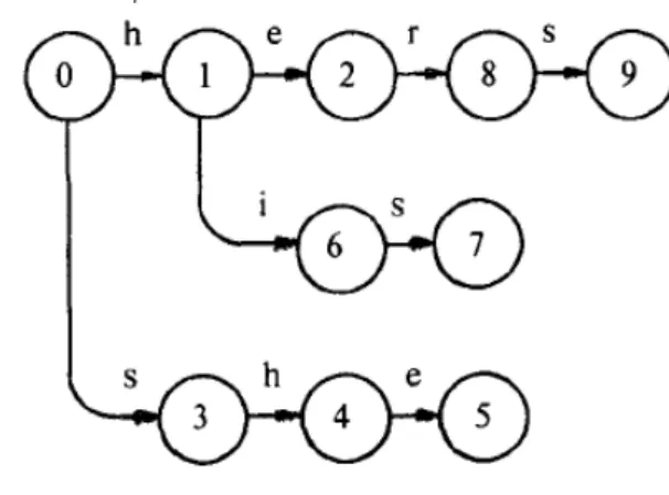
字串比對狀態機的建構例子如下，利用{he, she, his, hers }這一組關鍵字來 建造有限狀態機：首先設定start state是state 0，s代表current state，依照關鍵 字順序與字元順序依次加入goto graph，在current state如果沒有可以對應輸入 字元的transition存在，則我們增加一個新的state，它的編號是目前最大編號state number加1，並且用有向線從current state指向新增的state；若在current state 有可以對應輸入字元的transition，則沿著這個transition移動到下個state。首先 輸入第一個關鍵字he：

圖 2-1 goto graph 1

因為一開始已存在的狀態只有state 0所以在輸入”h”與”e”時都增加了新的state： state 1與state 2，即g(0,h)=1與g(1,e)=2，keyword輸入完畢，紀錄output(2)=”he”， 回到state 0。再來是第二個關鍵字she：

3 圖 2-2 goto graph 2

由於state 0並沒有對輸入字元”s”有可以transiton的state，所以輸入”s”、”h”、”e” 三個字元時都增加了新的state：state 3、state 4、state 5，即g(0,s)=3、g(3,h)=4 與g(4,e)=5，紀錄output(5)=”she”，回到state 0。再來是第三個關鍵字his：

圖 2-3 goto graph 3

因為state 0對輸入字元”h”有transition：g(0,h)=1，所以輸入”h”後current state變 成state 1，但是state 1對接下來的輸入字元”i”沒有transition，所以增加新state 6， 即g(1,i)=6，同理增加state 7，g(6,s)=7，output(7)=”his”，回到state 0，接著輸 入第四個關鍵字hers：

4

在輸入”h”和”e”時因為g(0,h)=1與g(1,e)=2，故我們不用新增state。但是在輸入”r” 與”s”時新增state 8與state 9，g(2,r)=8，g(8,s)=9，output(9)=”hers”。最後從state 0以一個有向線指向state 0表是沒有對應transition的所有字元都使狀態機停留在 state 0。

接下來處理failure function f(s)，首先定義state s的深度(depth)為goto graph 中從start state到state s的最短路徑之長，並且設定所有深度為1的state的f(s)=0。 深度為d的state的f(s)必須考慮所有深度為d-1的state r，如果存在輸入字元a使得 g(r,a)=s則設定state=f(r)，執行state←f(state)直到g(state,a)≠fail，則 f(s)=g(state,a)。由此我們可以得到f(1)=f(3)=0，f(2)=g(f(1),e)=g(0,e)=0， f(4)=g(f(3),h)=g(0,h)=1，f(6)=g(f(1),i)=g(0,i)=0，f(8)=g(f(2),r)=g(0,r)=0， f(7)=g(f(6),s)=g(0,s)=3，f(5)=g(f(4),e)=g(1,e)=2，f(9)=g(f(8),s)=g(0,s)=3。 圖 2-5 failure function

接著是完成 output function，當我們在處理 failure function 時，當我們決定了 f(s)=s’ 時同時將 s’的 output 合併到 state s 的 output 中：

5

2.2 Banded-Row Format 簡介

當我們需要儲存一個 vector，而這個 vector 的前後有數個 0 的串列，這個時 候我們可以使用 Banded-Row format[4]來儲存這個 vector，Banded-Row format 從這 個 vector 中第一個非零的值開始儲存到最後一個非零的值，第一個非零值的 index 被記為 Start index，而這個被儲存的序列長度稱為 bandwidth，如果這個 vector 之 中非零的元素位置相當集中並且數量不多，這種情況下使用 Banded-Row format 儲存這個 vector 將可以得到優異的儲存空間壓縮效果。存取壓縮過的 vector 內的 元素，首先判斷元素的原始 index 是否落在 Start index 和 Start index+bandwidth-1 這個範圍內（有包含邊界），若不在範圍內，表示我們要存取的元素的值為零； 若在範圍內，我們要存取的元素的新 index 將會是：

在原始 vector 中的 index - Start index + 2

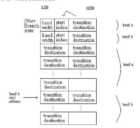
Banded-Row format 用在 Branch State 的例子如下：

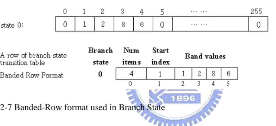
圖 2-7 Banded-Row format used in Branch State

State 0 是一個 Branch State，ASCII 碼 0 的字元使得狀態機停留在 State 0，ASCII 碼 1 的字元使得狀態機轉換到 State 1，ASCII 碼 2 的字元使得狀態機轉換到 State 2，ASCII 碼 3 的字元使得狀態機轉換到 State 8，ASCII 碼 4 的字元使得狀態機轉 換到 State 6，ASCII 碼 5 的字元使得狀態機停留在 State 0，… …，ASCII 碼 255 的字元使得狀態機停留在 State 0，總共需要 256 個單位的記憶體來儲存 State 0。 若是使用 Banded-Row format 來儲存這個 state 則只需 6 個單位的記憶體來儲存：1 個單位存 Bandwidth、1 個單位存 Start index、4 個單位存從第一個非零元素到最 後一個非零元素。

6

三、 網路安全應用可擴展字串比對架構的驗證模組

3.1 網路安全應用可擴展字串比對架構的簡介

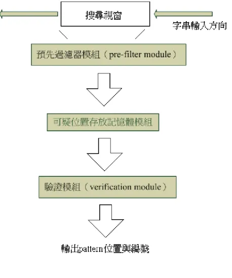
圖 3-1 string matching system architecure

如上圖，這是我們所提出的字串比對架構圖，字串比對系統將輸入的字串先 經過預先過濾器模組的過濾，將可疑的字串的起始位置紀錄在可疑位置存放記憶 體模組中，由驗證模組來檢查可疑字串是否與 pattern set 之中的 pattern 完全符合， 如果驗證的結果是完全符合則輸出該字串的位置與編號。整個系統分為兩個部份： 驗證模組與預先過濾器模組，以可疑位置存放記憶體模組為溝通的介面，分別由 我以及實驗室的另一位同學----李世宏所負責，下面是我所負責的驗證模組的介 紹。

7

在介紹驗證模組之前首先要對我們所提出來的網路安全應用可擴展字串比 對架構中用來儲存 state 資訊的資料結構與相關技術做簡單的介紹：

由 AC 演算法的 goto function 可以產生一個樹狀結構，在這個樹狀結構裡面的 state 依照所擁有的 next state 的數量不同可以分為三種，有兩個以上（包含兩個） next state 的 state 我們稱之為 Branch State，只有一個 next state 的 state 我們稱之為 Single-Child State，沒有 next state 的 state 我們稱之為 Leaf State。透過觀察我們發 現並不是所有 State 都有儲存的必要。我們定義了幾個新名詞：

Branch State：

擁有兩個或兩個以上 next states（children）的 state。 Single-Child State：

只有 1 個 next state 的 state。 First Single-Child State：

當一個 Single-Child State 的 parent state 是 Branch State 時我們稱它為 First Single-Child State。

Leaf State：

沒有 next state 的 state。 Explicit State：

當一個 state 屬於 root state、branch state、first single-child state 或 final state 我 們稱它為 Explicit State。

Nearest Descendent Explicit State(NDES)：

一個 state S 的所有後代（descendent）之中與 S 的距離最短，但是不為 S 的 Explicit State，我們稱它為 state S 的 NDES。

圖 3 要我 以不 3.2 分成 num 圖 3 下表 -2 explicit sta 如上圖， 我們將 patte 不必儲存， Double Ba 在我們的 成三組：Br mber＝1）， -3 stored state 雖然 Bran 表），但是

ate and non ex

任兩個相鄰 ern set 中的 這是資料結 anded-Row f 的驗證演算法 anch State（ Leaf State ( es nch State 的數 是單一 Branc xplicit state 鄰的 Explici pattern 用字 結構的壓縮 format 法中所有必 （children nu ( pattern is B 數量只有全 ch State 所必 8 it State 的中 字串的方式 縮與簡化。 必須儲存的 E umber＞1） Branch State 全部所必須儲 必須儲存的資 中間如果有非 式儲存起來 Explicit Stat ，Explicit S ) （children 儲存的 state 資訊卻遠高 非 Explicit S ，這些非 E tes 可經由 c Single-Child n number＝ e 數量的五分 高於 Single-C State 存在， xplicit State children 的數 d State（chil 0），如下圖 分之一左右 Child State 與 只 e 可 數量 ldren 圖： 右（見 與

9

Leaf State。若是要將 state transition table 儲存在實驗平台的內部記憶體中，Branch State 的記憶體消費問題是很明顯的。另一個困難在於不同 Branch State 之間的差 異相當大（這個差異的主要原因是 children number 的不同），使得單純使用一種 資料結構來儲存 Branch State 難以同時達到快速存取與節省記憶體空間這兩個目 的。Banded-Row format 雖然可以達到快速存取，但是在記憶體空間花費這方面的 表現卻不夠理想：

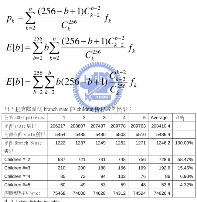
設 b 是 Banded-Row format 中的 Bandwidth，f_k 是 Branch State 有 k children 的 機率則 2 2 256 2 2 256 2 256 2 2

(256

1)

(256

1)

[ ]

b

C

p

f

C

b

C

E b

b

f

C

− +

=

− +

=

∑

∑ ∑

[ ]

(256

1)

C

E b

b

b

f

C

=

∑∑

− +

以下是實際量測 branch state 的 children 數目分佈情況：

任意 4000 patterns 1 2 3 4 5 Average 分佈 全部 state 數目 206217 208807 207487 209778 209763 208410.4 有儲存的 state 數目 5454 5485 5480 5503 5510 5486.4 全部 Branch State 數目 1222 1237 1249 1252 1271 1246.2 100.00% Children #=2 687 721 731 748 756 728.6 58.47% Children #=3 210 200 188 166 199 192.6 15.45% Children #=4 85 73 94 102 76 86 6.90% Children #=5 60 49 53 59 48 53.8 4.32% 記憶體花費(byte) 75468 74000 74828 74312 74524 74626.4 表 3. 1 state distribution table

上表為 pattern set 中任意 4000 pattern 做 5 次實驗所產生的結果，第二排為 4000 patterns 依照 AC 演算法所產生的 goto table 中全部 state 的數目。第三排為依照 我們所提出來的壓縮演算法所產生 goto table 中全部 state 的數目。第四排為第三

10

排的 state 之中屬於 Branch State 的總數，接下來的三排是 Branch State 之中 2-child、 3-child、4-child Branch State 的數目，最下一排是 Branch State 總共的記憶體花費。 Average 欄是前面五次量測的平均，分佈這欄表示了 2-child、3-child、4-child、 5-child Branch State 占全部 Branch State 數量的百分比。

由上表可以看出 children number 越多的 state 的數量越少，這完全與直觀相符

合。將實驗所得的數據套入 f_k ，k=2,3,4，k=5 之後的 f_k 以 0 代入可以得出 E[b]

的近似值：81.4 個單位。

在研究 ml310 這個實驗平台後我設計了一個資料結構：Double Banded-Row format。用 Double Banded-Row format 儲存 Branch State 不但可以擁有 Banded-Row format 快速存取的優點，在記憶體空間花費的問題上也有相當大的進步。

Double Banded-Row format 的產生過程如下，首先將我們要儲存的 vector 轉換 成以 Banded-Row format 表示，再針對 band 裡面的任兩個相鄰的非零元素計算 index 的差值，以有最大差值的兩個相鄰非零元素為界分成前後兩個 band，並且 各自用 Banded-Row format 表示得到這個 vector 的 Double Banded-Row format。

由實驗結果可以觀察到在全部的 Branch State 中 children number=2 的 Branch State 大約佔了 60%，children number<5 的 Branch State 佔了超過 80%，盡量減少 children number=2、3、4 的 Branch State 的記憶體使用量將會讓整體的記憶體使用 量得到最大的進步。

我們還可以做更進一步的資料結構簡化，除了必須儲存的 bandwidth 欄位之 外，當原始的向量只有 3 或 4 個非零元素時，我們可以連續儲存他們的 index 與 元素值，進一步減少 memory 的使用量。

11

四、 實做細節

4.1 驗證模組方塊圖

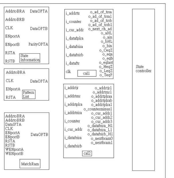
圖 4-1 verification module block diagram

各子模組功能說明如下：

State Information：存放所有 State 的資料結構。 Pattern List：存放所有 Pattern 的資料。

12

MatchRam：存放 true match 的 Pattern 編號與所在的位置。 State Controller：State 與 State 之間 transition 的控制。 cal1：

o_aHL = i_dataftr[0]~^i_datafsira[8]; o_bHL = i_dataftr[0]^i_datafsirb[8];

計算出一個 Branch State transition 的目的地是否紀錄在 band a 或是 band b 的高 位元部份，如果 input character 的 ASCII code 與 Double Banded-Row format 所 描述的 start index 同為奇數或偶數，則 o_aHL 會是 true value；反之 o_bHL 會 是 true value。

o_HeqZ = (i_datafsira[31:16] == 16'h0000)?1'b1:1'b0; o_LeqZ = (i_datafsira[15: 0] == 16'h0000)?1'b1:1'b0;

若一個 goto transition 的目的地是 0 表示在這個 Branch State 並沒有對應 input character 的 transition。

o_TeqP = (i_datafplra == i_dataftr)?1'b1:1'b0;

Current state 為 Single-Child State 時比較 input character 與 pattern 一致。

o_CeqZ = (i_counter == 7'b0000000)?1'b1:1'b0;

Current state 為 Single-Child State 時計算 loop counter 是否已經歸零

o_ad_of_trsb <= i_datafsirb[31:16] + ((i_dataftr – i_datafsirb[15:8])>>1);

若這個 Branch State transition 是由 b port 讀取出來，o_ad_of_trsb 會輸出紀錄 transition 目的地的欄位所在的位址。

o_ad_of_trsb1 <= i_datafsirb[31:16] + 1 + ((i_dataftr – i_datafsirb[15:8])>>1); 同上，但是位址前進 1。

o_ad_of_trsa <= i_cur_addr + ((i_dataftr - i_datafsira[15:8] + 3)>>1);

若這個 Branch State transition 是由 a port 讀取出來，o_ad_of_trsa 會輸出紀錄 transition 目的地的欄位所在的位址。

o_ad_of_trsa1 <= i_cur_addr + ((i_dataftr - i_datafsira[15:8] + 5)>>1); 同上，但是位址前進 1。

13

( (i_dataftr>=i_datafsira[15:8])&&(i_dataftr<=(i_datafsira[15:8]+i_datafsira[7:0])) )?1'b1:1'b0;

若這個 Branch State transition 是由 a port 讀取出來，o_ain 將判斷 input character 是否落在 bandwidth 之內。

o_bin <=

( (i_dataftr>=i_datafsirb[15:8])&&(i_dataftr<=(i_datafsirb[15:8]+i_datafsirb[7:0])) )?1'b1:1'b0;

若這個 Branch State transition 是由 b port 讀取出來，o_bin 將判斷 input character 是否落在 bandwidth 之內。

o_eqa <= (i_dataftr == i_datafsira[15:8])?1'b1:1'b0;

o_eqa 判斷 input character 是否與 band a 的 start index 相等。

o_eqb <= (i_dataftr == i_datafsirb[15:8])?1'b1:1'b0;

o_eqb 判斷 input character 是否與 band b 的 start index 相等。

o_eqlast <= (i_addrttr == 13'b1111111111111)?1'b1:1'b0; o_eqlast 判斷 text 的指標是否達到 text 的尾端。

o_next_ch_ad 計算下個 input character 的位址。 cal2： o_cur_addr1=i_cur_addr+1; 計算出 current address+1 o_cur_addr2=i_cur_addr+2; 計算出 current address+2 o_cur_addr3=i_cur_addr+3; 計算出 current address+3 o_datafsira_H1=i_datafsira[31:16]+1;

由 State Information 模組 a port 所輸出的高位元部份的 transition address+1 o_datafsira_L1=i_datafsira[15:0]+1;

14

o_datafsirb_H1=i_datafsirb[31:16]+1;

由 State Information 模組 b port 所輸出的高位元部份的 transition address+1 o_addrtmr1=i_addrtmr+1;

計算下個 MatchRam 可以寫入的位址。 o_addrtjr1=i_addrtjr+1;

計算下個 verification request 的位址。

o_addrtplraa=i_datafsira[31:14]+i_datafsira[13:7];

計算對應 input character，pattern 內的字元的位址，i_datafsira[31:14]與 i_datafsira[13:7]將由 State Information 模組的 port a 提供。

o_addrtplrab=i_datafsirb[31:14]+i_datafsirb[13:7];

計算對應 input character，pattern 內的字元的位址，i_datafsirb[31:14]與 i_datafsirb[13:7]將由 State Information 模組的 port b 提供。

o_addrtplra1=i_addrtplra+1;

計算 Pattern List 模組中下個字元的位址。

o_nextbram0={i_addrtsira[15:9],9'b000000000}+16'h0200; 計算 State Information 模組內下個 bram 的開始位址。 o_nextbram1={i_addrtsira[15:9],9'b000000000}+16'h0201; 同上，位址加 1。

o_counterminus1=i_counter-1; 計算 counter 減 1 的值。

15

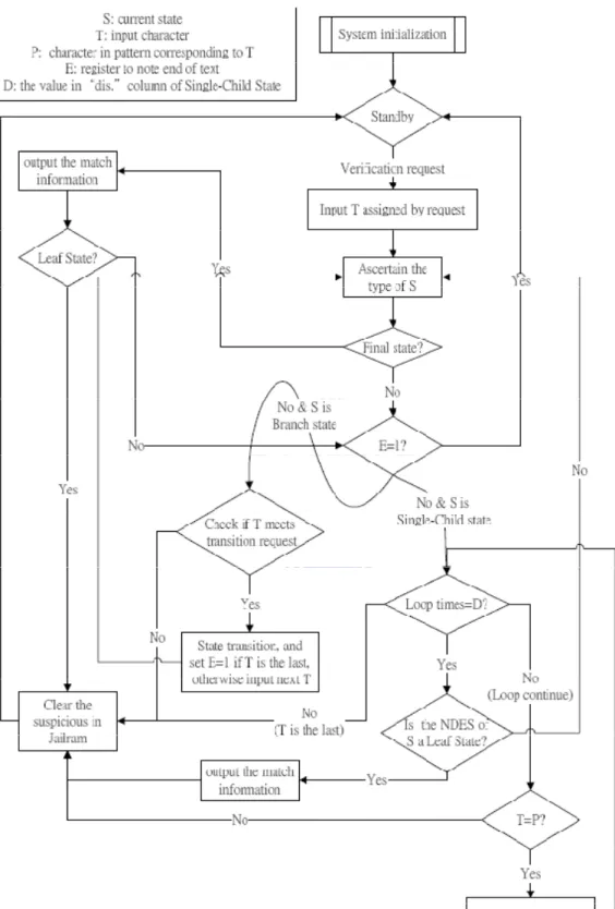
4.2 驗證模組工作流程

16

驗證演算法： //system initialization S: current state T: input character

P: character in pattern corresponding to T E: register to note end of text

D: the value in "dis." column of Single-Child State while( !(pre-filter end signal) )

{

while( !(verification request) ) { standby; }

S←0;

Input T assigned by request; while( )

{

if(S is final state) {

Output the match information; if(S is Leaf State)

{

Clear the suspicious in JailRam; break;

} }

if(E==1)

{ break; } if(S is Branch State) {

if(T meets transition request) {

if(T is the last) { Set E=1; } else { Input next T; } } else {

Clear the suspicious in JailRam; break;

} }

else //S is Single-Child State {

for(counter=D;counter>0;counter--) {

if( (T!=P) or (T is the last) ) {

Clear the suspicious in JailRam; break;

}

Get next T and next P; }

17

{

Output the match information; Clear the suspicious in JailRam; break; } } S←Next State; } }

4.3 各種資料結構與 Next State transition 機制說明

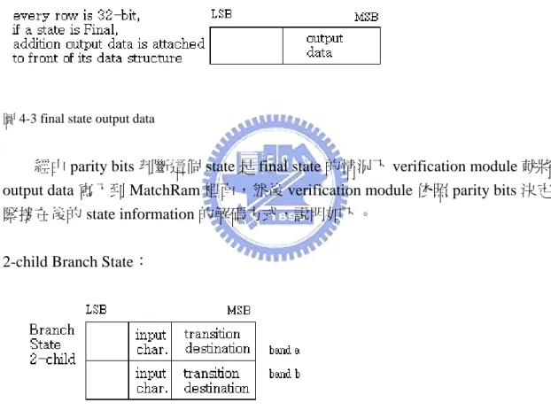
在所有被儲存的 state 中，如果該 state 是 final state 則該 state 的資料結構會 附加 output data 在原本的資料結構前方如下圖：

圖 4-3 final state output data

經由 parity bits 判斷這個 state 是 final state 的情況下 verification module 就將 output data 寫入到 MatchRam 裡面，然後 verification module 依照 parity bits 決定 緊接在後的 state information 的解碼方式，說明如下。

2-child Branch State：

圖 4-4 data structure of 2-child Branch State

Double Banded-Row format 中第一個欄位是 Bandwidth(占 8 bits)，由於原始 vector 只有 2 children，所以在分成兩個 band 之後，兩個 Bandwidth 欄位應該都 是 1，但是經由 parity bits 即可判斷這個 state 是 2-child Branch State，所以這欄位 在這種情況下沒有實際功能，保存目的是為了使所有 Branch State 的解碼元件可 以盡量共用。

18

資料候可以得知 current state 對此 input character 有沒有 transition，若有，則 current state 指向後面的 transition destination 欄位(占 16 bits)所紀錄的 next state address。

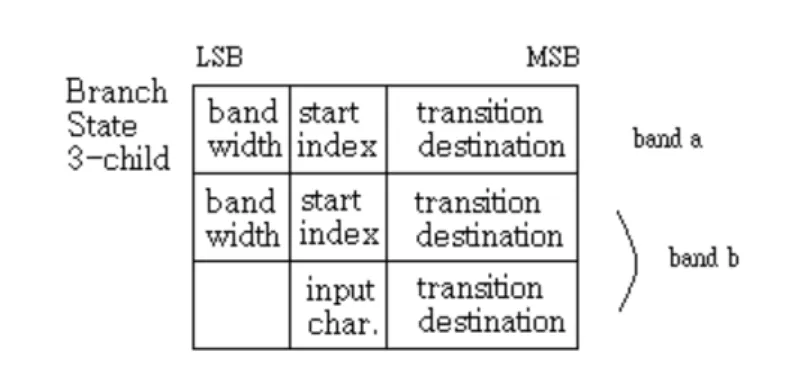
3-child Branch State：

圖 4-5 data structure of 3-child Branch State

由於原始 vector 有 3 children，所以在分成兩個 band 之後，其中一個 band 的 Bandwidth 將會是 1，這個 band 的資料將被紀錄在圖中最上面的 row，另一個 band 將會有 2 children，分別紀錄在中間與下面這兩 row，與 2-child Branch State 不同的地方在於這個 band 的 Bandwidth 欄位是有意義的，經由 parity bits 判斷這 個 state 是 3-child Branch State 之後，Bandwidth 欄位使得 verification module 可以 快速的判斷從 TextRam 取得的 character 是否在 band 之外，若否，則與 start index 和 input char.這兩個欄位做比較得知是否有 transition。

4-child Branch State：

圖 4-6 data structure of 4-child Branch State

由於原始 vector 有 4 children，在分成兩個 band 之後可能會出兩種情況。一、 其中一個 band 只有 1 child，而另一個 band 有 3 children。二、兩個 band 各擁有

19

2 children。如果是第一種情況，Bandwidth＝1 的 band 的資料將被紀錄在圖中最 上面的 row，擁有 3 children 的 band 的資料將被紀錄在下面三個 row，圖中這兩 個 Bandwidth 欄位都是有功能的，可以幫助判斷從 TextRam 取得的 character 是 否在 band 之外，若否，則與 start index 和 input char.這兩個欄位做比較得知是否 有 transition；如果是第二種情況，其中一個 band 的第 1 個元素將被紀錄在第 1 個 row，第 2 個 row 紀錄另一個 band 的第一個元素，剩下的兩個元素分別放在 下面的兩個 row，Next State transition 機制與 3-child Branch State 同樣。

Over 4-child Branch State：

圖 4-7 data structure of over 4-child Branch State

在原始的 vector 被分成兩個 band 之後，兩個 band 各自的第一個元素將被 存放在第一與第二個 row，如上圖，從第三個 row 開始存放的是 band a 剩下來 的元素，緊接在後的事 band b 剩下來的元素。與前三種資料結構不同的是第二 個 row 的 transition destination 欄位放的位址並不是 start index 這個元素的 transition destination，而是 band b 的 start address，這是因為 band a 的 Bandwidth 並不是一個定值的緣故。在確定從 TextRam 取得的 character 在哪個 band 內之後， 一個暫時的指標指向 cal1 模組所產生的 o_ad_of_trsa(或 o_ad_of_trsb)的值，並由 o_aHL 或 o_bHL 確定 transition destination 是在高位元部份還是低位元部份讀取 next state 位址。 

20

在此可以透過上面的實驗數據表中的平均記憶體花費來計算 Double 

Banded‐Row format Bandwidth 的近似值，因為 transition destination 欄占 16 bits， 所以必須將以 byte 為單位的平均記憶體花費除以 2，再來扣除每個 Branch State 皆有兩單位的 overhead 與 Over 4-child Branch State 資料結構可能有的空白欄位 （假設兩個 band 之後有空白的機率各 50%）： 

( 74626.4/2 - 2*1246.2 – 1246.2*(100% - 58.47% -

15.45%*-6.90%)*(0*0.25+2*0.25+1*0.5))/ 1246.2 ~= 27.75 個單位。大約是單純使 用 Banded-Row format 的 1/3。

Explicit Single-Child State：

圖 4-8 data structure of Explicit Single-Child State  

Explicit Single-Child State 由三個欄位組成：dis.(distance，占 7 bits)、 pos.(position，占 7 bits)、pattern start addr.(pattern 開始的位址，占 18 bits)，經由 parity bits 判斷這個state 是 Explicit Single-Child State 之後，dis.的值將被 counter 所紀錄，而 pos.與 pattern start addr.這兩個欄位的值將會透過 cal2 模組產生對應 input character、該 pattern 內的字元的位址。透過連續的比較來決定 next state 的 走向（詳見 verification flow chart）。

Leaf State(parent is Branch State)：

圖 4-9 data structure ofLeaf State (parent is Branch State) 

由於 Leaf State 是 final state 的其中一類、並且不會 transition 到任何其他的 state，Leaf State 的資料結構將與圖 4‐3 一模一樣，output data 欄位占 18 bits。在

21

parity bits 的判斷後 verification module 可以知道 Explicit Single‐Child State 的 NDES 是否是 Leaf State，進而輸出 pattern match 或是前進到下一個 state，所以 parent  state 是 Explicit Single‐Child State 的 Leaf State 是不需要儲存的。但是 Branch State 由於欄位寬度的因素並不能將 Leaf State 的 output data 全部儲存，所以這種情況 下的 Leaf State 必須額外花費空間來儲存 output data，而 Branch State 的欄位填 入 transition address 來指向這個 Leaf State，不過這種情況出現的機率是相當低的， 根據多次實驗觀察大約是所有儲存的 state 數量的 0.001。 

22

五、 數據與效能

5.1 實驗環境介紹

我們的病毒碼來源是 ClamAV [5]。系統運行平台為 Xilinx Vertex-II Pro ML310 Platform 如下圖，我們的硬體設計在此平台的 on-board Xilinx Virtex II Pro (XCVP30) FPGA 之內。

圖 5-1 Xilinx Vertex-II Pro ML310 Platform

23 圖 5-3 block ram configuration 2 ports

圖 5-4 block ram configuration 1 port

如圖 5-3 與圖 5-4，block ram 可以有多種配置的選擇，在驗證模組(verification module) 中 State Information、MatchRam 是使用 RAMB16_S36_S36 的配置，Pattern List 是使 用 RAMB16_S9 的配置

24 5.2 效能 以下是排除預先過濾器模組（pre-filter module）的加速功能，單純測驗證模 組（verification module）throughput 的實驗結果，實際上驗證模組是不能在沒有預 先過濾器模組的情況下單獨運作，量測方式說明如下：首先任意選擇幾個 pattern 將它們串聯起來填滿被掃瞄的 text 所存放的區域，開始掃描之前就將每個 pattern 的起始位置記錄在 JailRam 之中，然後整個系統開始運作，量測開始與結束的時 間差。變換不同 pattern 與其數量測量數次，取平均值。這樣一來包括狀態機的 traverse 時間、pattern address 讀取時間都ㄧ並量測到了，也排除預先過濾器模組 的效果。而整個系統構造跟有預先過濾器模組一起參與工作的情況基本上是一樣 的。

以下的系統工作頻率皆為 135.14MHz

4000 pattern set avg. length = 29 Byte 開始時間 (ns) 結束時間 (ns) 執行時間(ns) Pattern 數量 平均長度(B) Throughput(Mb/s) 216 164725.2 164509.2 284 28.7394 396.91 216 166086.0 165870.0 290 28.1793 394.14 216 163234.8 163018.8 276 29.5833 400.69 216 164264.4 164048.4 284 28.7359 397.98 216 163702.8 163486.8 277 29.4657 399.4 216 165934.8 165718.8 287 28.4913 394.74 216 162831.6 162615.6 276 29.5978 401.88 216 162406.8 162190.8 274 29.8066 402.83 216 162817.2 162601.2 283 28.8163 401.23 216 161874.0 161658.0 274 29.8212 404.36 Avg.=163571.76 Avg.=399.42

表 5. 1 throughput without pre-filter work

以下是加入預先過濾器模組的功能掃描一個乾淨的文件的 throughput： 開始時間 (ns) 結束時間 (ns) 執行時間(ns) Pattern 數量 平均長度(B) Throughput(Mb/s) 216 36845.7 36629.7 0 0 1789.15

25 以下是加入預先過濾器模組的功能掃描一個內含 10 個 pattern 的文件的 throughput： 開始時間 (ns) 結束時間 (ns) 執行時間(ns) Pattern 數量 平均長度(B) Throughput(Mb/s) 216 38306.6 38090.6 10 23.5 1720.53

表 5. 3 throughput with pre-filter scan text contain 10 patterns

驗證模組系統資源使用：

Synthesis tool: XST(VHDL/Verilog)

Logic Utilization Used Available Utilization

Number of Slices 1617 13696 11% Number of Slice Flip Flops 404 27392 1% Number of 4 input LUTs 3151 27392 11% Number of bonded IOBs 98 556 17%

Number of BRAMs 106 136 77%

Number of GCLKs 1 16 6%

表 5. 4 verification module resource usage

總共儲存了 4000 個 pattern，平均 pattern 長度= 29 Byte。 1 Bram 可以儲存 2^14 bits = 2048 bytes.

26

全系統（包含預先過濾器模組）的資源使用： Synthesis tool: XST(VHDL/Verilog)

Logic Utilization Used Available Utilization

Number of Slices 1825 13696 13%

Number of Slice Flip Flops 460 27392 1%

Number of 4 input LUTs 3532 27392 12%

Number of bonded IOBs 46 556 8%

Number of BRAMs 119 136 87%

Number of GCLKs 1 16 6%

表 5. 5 whole system resource usage

總共儲存了 4000 個 pattern，平均 pattern 長度= 29 Byte。 1 Bram 可以儲存 2^14 bits = 2048 bytes.

27

六、 結論

我們在 ML310 這個實驗平台上實現了一個高速並且記憶體資源消耗低的字 串比對系統，整個系統的 throughput 可超過 1.7Gbps，並且可以針對輸入文章同 時進行 4000 個 pattern 的比對，並且輸出 pattern 在文章中的位址。

Double Banded-Row format 是一個基於 Banded-Row format 而改良出來的資料 壓縮格式，它在具備 Banded-Row format 的簡單存取的優點之外還可以使記憶體 資源消耗減少大約 2/3。

28

參考文獻

[1] R. S. Boyer and J. S. Moore. “A Fast String Searching Algorithm,”Comm. Of the

ACM, vol. 20, issue 10, pp.762-772, Oct. 1977.

[2] D. Knuth, J. Morris and V. Pratt, “Fast pattern matching in strings,”

TRCS-74-440, Stanford University, Stanford California, 1974.

[3] A. Aho and M. Corasick, “Efficient string matching: An aid to bibliographic

search,”Comm. Of the ACM, vol. 18, issue 6, pp.333-343, Jun. 1975.

[4] M. Norton, “Optimizing Pattern Matching for Intrusion Detection,” Available:

http://www.snort.org/docs/

29

附錄

合成器 Synthesize 結果：

使用 Xilinx ISE 8.1i 內建合成器（Synthesizer）

1 僅驗證模組

Timing Summary: --- Speed Grade: -6

Minimum period: 7.071ns (Maximum Frequency: 141.433MHz) Minimum input arrival time before clock: 7.669ns

Maximum output required time after clock: 3.839ns Maximum combinational path delay: No path found

Timing Detail: ---

All values displayed in nanoseconds (ns)

========================================================================= Timing constraint: Default period analysis for Clock 'clk'

Clock period: 7.071ns (frequency: 141.433MHz) Total number of paths / destination ports: 54348 / 1019 --- Delay: 7.071ns (Levels of Logic = 15) Source: siBR/DataOPTA_8 (FF) Destination: cal1/o_ad_of_trsa_14 (FF)

30

Source Clock: clk rising Destination Clock: clk rising

Data Path: siBR/DataOPTA_8 to cal1/o_ad_of_trsa_14 Gate Net

Cell:in->out fanout Delay Delay Logical Name (Net Name) --- ---

FD:C->Q 9 0.374 0.703 siBR/DataOPTA_8 (siBR/DataOPTA_8) LUT2_L:I1->LO 1 0.313 0.000 cal1/CAL1__n0008<0>lut1 (N4950)

MUXCY:S->O 1 0.377 0.000 cal1/CAL1__n0008<0>cy (cal1/CAL1__n0008<0>_cyo) XORCY:CI->O 14 0.868 0.792 cal1/CAL1__n0008<1>_xor (cal1/CAL1__n0005<1>_sel) LUT2_D:I0->O 2 0.313 0.495 cal1/CAL1__n0003<4>cy1_SW0 (N4904)

LUT4:I3->O 1 0.313 0.440 cal1/CAL1__n0003<4>cy1 (cal1/CAL1__n0003<4>_cyo) LUT4_L:I3->LO 1 0.313 0.000 cal1/CAL1__n0011<6>lut (cal1/N114)

MUXCY:S->O 1 0.377 0.000 cal1/CAL1__n0011<6>cy (cal1/CAL1__n0011<6>_cyo) MUXCY:CI->O 1 0.041 0.000 cal1/CAL1__n0011<7>cy (cal1/CAL1__n0011<7>_cyo) MUXCY:CI->O 1 0.041 0.000 cal1/CAL1__n0011<8>cy (cal1/CAL1__n0011<8>_cyo) MUXCY:CI->O 1 0.041 0.000 cal1/CAL1__n0011<9>cy (cal1/CAL1__n0011<9>_cyo) MUXCY:CI->O 1 0.041 0.000 cal1/CAL1__n0011<10>cy (cal1/CAL1__n0011<10>_cyo) MUXCY:CI->O 1 0.041 0.000 cal1/CAL1__n0011<11>cy (cal1/CAL1__n0011<11>_cyo) MUXCY:CI->O 1 0.041 0.000 cal1/CAL1__n0011<12>cy (cal1/CAL1__n0011<12>_cyo) MUXCY:CI->O 0 0.041 0.000 cal1/CAL1__n0011<13>cy (cal1/CAL1__n0011<13>_cyo) XORCY:CI->O 1 0.868 0.000 cal1/CAL1__n0011<14>_xor (cal1/_n0011<14>)

FD:D 0.234 cal1/o_ad_of_trsa_14 ---

Total 7.071ns (4.641ns logic, 2.430ns route) (65.6% logic, 34.4% route)

31

2 全系統（預先過濾器模組與驗證模組一起）

Timing Summary: --- Speed Grade: -6

Minimum period: 7.226ns (Maximum Frequency: 138.389MHz) Minimum input arrival time before clock: 3.742ns

Maximum output required time after clock: 6.516ns Maximum combinational path delay: No path found

Timing Detail: ---

All values displayed in nanoseconds (ns)

========================================================================= Timing constraint: Default period analysis for Clock 'clk_p'

Clock period: 7.226ns (frequency: 138.389MHz) Total number of paths / destination ports: 73115 / 1227 --- Delay: 7.226ns (Levels of Logic = 8) Source: acv4/cur_state_2_1 (FF) Destination: acv4/AddrTsiRB_9 (FF) Source Clock: clk_p rising

Destination Clock: clk_p rising

Data Path: acv4/cur_state_2_1 to acv4/AddrTsiRB_9 Gate Net

32

Cell:in->out fanout Delay Delay Logical Name (Net Name) --- ---

FDRS:C->Q 1 0.374 0.533 acv4/cur_state_2_1 (acv4/cur_state_2_1) LUT2_D:I0->O 18 0.313 0.726 acv4/Ker1811 (acv4/N1811)

LUT4:I2->O 1 0.313 0.533 acv4/Ker1481_2 (acv4/Ker14811) LUT4_L:I0->LO 1 0.313 0.000 acv4/Ker146_G (N6217)

MUXF5:I1->O 5 0.340 0.531 acv4/Ker146 (acv4/N146) LUT3_D:I2->O 6 0.313 0.552 acv4/Ker6922 (acv4/N69) LUT4:I2->O 10 0.313 0.717 acv4/Ker381_3 (acv4/Ker381_11)

LUT3:I1->O 2 0.313 0.495 acv4/_n0043<9>43 (acv4/_n0043<9>_map2978) LUT4_L:I3->LO 1 0.313 0.000 acv4/_n0043<9>60 (acv4/_n0043<9>)

FDS:D 0.234 acv4/AddrTsiRB_9 ---

Total 7.226ns (3.139ns logic, 4.087ns route) (43.4% logic, 56.6% route)