國 立 交 通 大 學
電子工程學系 電子研究所碩士班
碩 士 論 文
用於 UWB 及 WIMAX 之雙模
通道等化器設計
Dual mode Channel Equalizer Design
for UWB and WIMAX Systems
研 究 生:葉柏麟 Po-Lin Yeh
指導教授:溫瓌岸 博士 Dr. Kuei-Ann Wen
用於 UWB 及 WIMAX 之雙模
通道等化器設計
Dual mode Channel Equalizer Design
for UWB and WIMAX Systems
研 究 生:葉柏麟
Student: Po-Lin Yeh
指導教授:溫瓌岸 博士
Advisor: Dr. Kuei-Ann Wen
國 立 交 通 大 學
電子工程學系 電子研究所碩士班
碩 士 論 文
A Thesis
Submitted to Department of Electronics Engineering & Institute of
Electronics
Electronics College of Electrical and Computer Engineering
National Chiao Tung University
in Partial Fulfillment of the Requirements
for the Degree of Master
in
Electronic Engineering
July 2008
i
於 UWB 及 WIMAX 之雙模
通道等化器設計
研究生:葉柏麟 指導教授: 溫瓌岸博士
國立交通大學 電子工程學系 電子研究所碩士班摘要
本論文提出一適用於 IEEE 802.15.3a 與 IEEE 802.16d 雙規格的通道等化器, 此通道等化器包含通道估測,頻域等化器,相位追蹤器,適應性通道追蹤器等, 用以解決正交分頻多工系統上,存在之多路徑通道,加成性白色高斯,射頻傳輸 器與接收器之本地訊號不匹配以及D/A 與 A/D 之取樣頻率不匹配等非理想效應。 經由完整的 UWB 系統模擬,所提出的方法在不同的傳輸環境下,可達到 1.36~7.25dB 的 SNR 系統效能增益,WIMAX 的系統方面,另提出的適應性通道 追蹤器,可有效減少通道估測誤差,經由模擬,提出的方法可降低3~18 dB 的通 道估測方均誤差(MSE),在不同的傳輸環境下,也可獲得 0.5~3.9dB 的 SNR 系統 效能增益。 為了處理雙模的訊號,採用了通用於兩種系統規格的演算法,電路設計上得 以運用通用的運算單元,以提升使硬體使用效率,藉由Synopsys Design Complier 合成,在UMC 0.18 um CMOS 的製程環境下,所提出的設計僅需 13 萬邏輯閘, 另外為了符合UWB 528Msamples/s 的資料處理速度,電路上採用了兩倍平行度
ii
Dual mode Channel Equalizer Design
for UWB and WIMAX Systems
Student: Po-Lin Yeh Advisor: Dr. Kuei-Ann Wen
Department of Electronics Engineering Institute of Electronics National Chiao-Tung University
Abstract
In this thesis, a dual mode channel equalizer is proposed for applications on IEEE 802.15.3.a and IEEE 802.16d. The proposed channel equalizer comprises channel estimator, frequency domain equalizer, phase error tracker, and adaptive channel tracker. It is applied to resolve non-ideal effects, such as multi-paths channel, additive white Gaussian noise, carrier frequency mismatch between RF transmitter and receiver, sampling clock mismatch between digital-to-analog converter and analog-to-digital converter in Orthogonal Frequency Division Multiplexing (OFDM) system.
Through complete UWB simulation, the proposed channel equalizer can obtain 1.36 ~7.25dB gain in signal-to-noise ratio (SNR) for different transmission conditions. In WIMAX system, the proposed adaptive channel tracker can reduce channel estimation error effectively. With system simulation, the proposed adaptive channel tracker can reduce the mean-square-error of channel estimation by 3~18 dB. Under
iii
different transmission conditions, the proposed methodology can obtain 0.5~3.9 dB SNR gain.
In order to deal with dual-mode signals, common algorithms are selected to process both UWB and WIMAX signals. With common Algorithms, common architectures can be designed to obtain hardware efficiency. Design is synthesized to UMC 0.18um CMOS standard cell technology library with Synopsys Design Compiler. The total gate count is merely 130k. Finally, in order to meet the sampling rate of 528Msample/s for UWB, the proposed channel equalizer uses two-parallelism and throughput can achieves 540M samples per second.
iv
誌 謝
首先,第一個要感謝的是指導教授,溫瓌岸教授。感謝老師在兩年研究生涯 中,不斷的給予柏麟指導與督促。溫老師的教誨,讓學生在學習訓練的路途上, 能夠快速而正確的修正自己的研究方向,並且保持不鬆懈的心態進行研究,也感 謝TWT_LAB 在這兩年中提供的豐富研究資源,讓我在研究上無後顧之憂,感 謝實驗室的學長們的指導與照顧:彭嘉笙,溫文燊,林立協,陳哲生,鄒文安, 廖俊閔,張懷仁,蔡彥凱,莊翔琮,林義凱,吳家岱,梁書旗,李漢建,侯閎仁。 感謝兩年來一起打拚的同學:黃俊彥,黃謙若,楊士賢,林佳欣,黃國爵,王磊 中。大家在生活上的互相扶持與鼓勵,讓原本辛苦煩悶的研究工作,也變的輕鬆 愉快許多。 同時也要感謝實驗室的助理:翁淑怡,陳宛君,張嘉誠,魏智伶,陳恩齊, 陳慶宏,有妳們幫忙處理實驗室的雜務,才能讓我們能夠專心致力於研究。感謝 默默支持我的家人,爸爸,媽媽,哥哥。你們不斷的支持與鼓勵,讓我覺得需要 更努力來回報你們。最後,感謝可愛與聰明的女朋友先俐,陪我度過兩年的歲月. 葉柏麟 2008 年 7 月v
Contents
摘要 ... i
Abstract ... ii
誌 謝 ...iv
List of Tables ...vi
List of Figures ... vii
Chapter 1. Introduction ... 1
1.1. Motivation ... 1
1.2. Introduction to OFDM system... 2
1.3. Introduction to Multi-Band OFDM Ultra Wide Band ... 5
1.3.1. UWB physical layer ... 5
1.4. Introduction to IEEE 802.16d Fixed WIMAX ... 9
1.4.1. Fixed-WIMAX physical layer ... 9
1.5. Channel Equalizer Design Spec ... 12
Chapter 2. Design Specification of Dual-Mode Channel Equalizer ... 13
2.1. Wireless Channel Model ... 13
2.2. Intel Proposed UWB Multi-paths Channel Model ... 13
2.3. WIMAX SUI Channel Model ... 19
2.4. Carrier Frequency Offset Model ... 24
2.5. Sampling Clock Offset Model ... 25
2.6. Additive White Gaussian Noise ... 27
Chapter 3. Design of Dual-Mode Channel Equalizer ... 28
3.1. Dual-Mode Design of Channel Estimation ... 29
3.1.1. Channel Estimation for UWB ... 30
3.1.2. Channel Estimation for WIMAX ... 31
3.2. Dual-Mode Design of Equalization ... 33
3.3. Dual-Mode Design of Phase Error Tracking and compensation ... 34
3.4. Modified-NLMS Channel Tracking ... 37
Chapter 4. Simulation Result and Performance Analysis ... 40
4.1. Performance Analysis of the Proposed Dual-Mode Channel Equalizer for UWB system ... 40
4.2. Performance Analysis of the Proposed Dual-Mode Channel Equalizer for WIMAX system ... 44
vi
Chapter 5. Hardware Implementation ... 49
5.1. Signal Flow of Dual-Mode Channel Equalizer ... 49
5.2. Architecture of Dual-Mode Channel Estimator ... 51
5.3. Architecture of Dual-Mode Equalizer ... 54
5.4. Architecture of Dual-Mode Phase Error Tracker and Compensator ... 56
5.5. Architecture of Modified-NLMS Channel Tracker ... 59
5.6. Architecture of Dual-Mode Channel Equalizer ... 60
5.7. Implementation Issues ... 61
5.8. Hardware Implementation Results ... 61
For WIMAX application, system clock rate is 50MHz and the power consumption of dual-mode channel equalizer is 47.38mW. For UWB application, clock rate is 270 MHz, and corresponding power consumption is 72.56 mW. ... 62
5.9. FPGA Prototyping ... 63
5.10. FPGA Emulation... 65
Chapter 6. Conclusions and Future Work ... 67
6.1. Conclusions ... 67
6.2. Future Work ... 67
Bibliography ... 68
List of Tables
Table 1.1 – Rate-dependent parameters for UWB ………7Table 1.2 – Timing-related parameters for UWB...………7
Table 1.3 –Timing related parameters for WIMAX ………...9
Table 1.4 –Available bandwidth list for WIMAX………10
Table 1.5 –Seven different transmission types for WIMAX………....10
Table 2.1 –Parameter Settings for the IEEE UWB Channel Model………17
Table 2.2 – SUI Channel...19
Table 2.3 – SUI Channel Parameters………...………….21
Table 4.1 – Performance Result for UWB system………...43
Table 4.2 –Performance Result for WIMAX system………...48
Table 5.1 – Relationship of operation in single iterative unit………..55
Table 5.2 – Synthesis Report for Each Module………62
vii
List of Figures
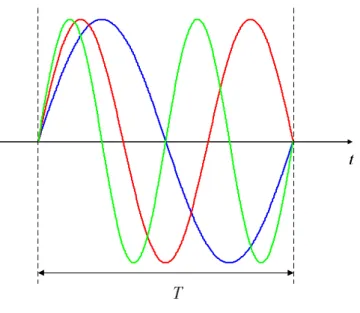
Fig. 1.1 Example of three orthogonal sub-carriers within one OFDM symbol………..3
Fig. 1.2 Overlapped orthogonal sub-carriers………..3
Fig. 1.3 OFDM symbol………..4
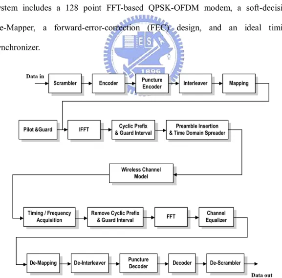
Fig. 1.4 Block Diagram of Baseband Transceiver………..5
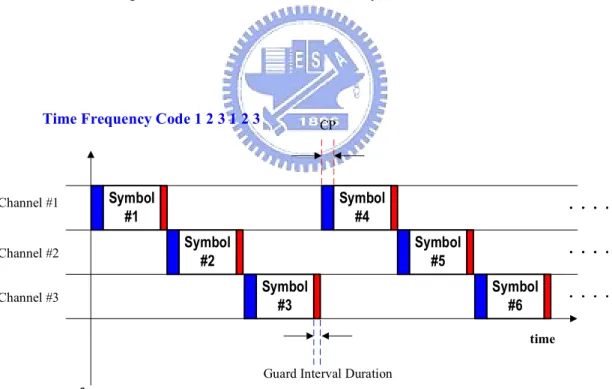
Fig. 1.5 TFC Example of UWB……….6
Fig. 1.6 UWB Frame Format……….8
Fig. 1.7 WIMAX Frame Format………...11
Fig. 2.1 CIR, CFR of the CM2 and CM4……….18
Fig. 2.2 CIR and CFR for SUI-1………..22
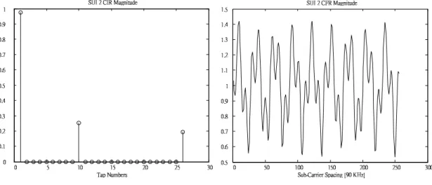
Fig. 2.3 CIR and CFR for SUI-2………..23
Fig. 2.4 CIR and CFR for SUI-3………..23
Fig. 2.5 ICI effect……….24
Fig. 2.6 SCO effect………...25
Fig. 2.7 FIR filter structure………...26
Fig. 2.8 Sampled value of the raised cosine function………...26
Fig. 3.1 Block Diagram of Proposed Channel Equalizer……….28
Fig. 4.1 PER (%) simulation for different SNR and CFO, SCO value under CM2, data rate 480Mb/s……….41
Fig. 4.2 PER (%) simulation result with different CFO, SCO value in CM2………..41
Fig. 4.3 PER (%) simulation result for different data rates in AWGN channel with 40 ppm of CFO, SCO value………..42
Fig. 4.4 PER (%) simulation result for different data rates and channel model with 40 ppm of CFO, SCO value………..42
Fig. 4.5 MSE analysis of Modified-NLMS channel tracker………....44
Fig. 4.6 Channel Estimation Error from sub-carrier number 70 to 110………...45
Fig. 4.7 Learning Curve for modified-NLMS channel tracker………45
Fig. 4.8 BER Comparison………46
Fig. 4.9 BER performance under Bandwidth=20 MHz, CFO=0.1 ppm, SCO=16 ppm, SUI-1 channel……….47
Fig. 4.10 BER performance under Bandwidth=20 MHz, CFO=0.1 ppm, SCO=16 ppm, SUI-2 channel……….47
Fig. 4.11 BER performance under Bandwidth=20 MHz, CFO=0.1 ppm, SCO=16 ppm, SUI-3 channel……….48
viii
Fig. 5.2 Signal Flow of Proposed Channel Equalizer for WIMAX……….50
Fig. 5.3 Architecture of proposed dual-mode channel estimator……….51
Fig. 5.4 Architecture of noise power estimator………52
Fig. 5.5 Architecture of 6-tap raised-cosine interpolator………..53
Fig. 5.6 Operation of 6-tap raised-cosine interpolator……….53
Fig. 5.7 Architecture of dual-mode equalizer………...54
Fig. 5.8 Architecture of pipelined real divider……….55
Fig. 5.9 Architecture of dual-mode phase error tracker and compensator…………...57
Fig. 5.10 Architecture of pipeline cordic………..58
Fig. 5.11 Architecture of modified-NLMS channel tracker……….59
Fig. 5.12 Architecture of Dual-Mode Channel Equalizer………60
Fig. 5.13 Fixed Point Simulation……….…61
Fig. 5.14 FPGA verification plan……….63
Fig. 5.15 FPGA Board………..64
Fig. 5.16 Synthesis Report for 12x64 bits of Register file………...64
Fig. 5.17 Synthesis Report for 12x256 bits of Register file……….64
Fig. 5.18 Synthesis Report of Dual-Mode Channel Equalizer……….…65
Fig. 5.19 FPGA Emulation………...65
Fig. 5.19 RTL Simulation………..………...66
Fig. 5.21 FPGA Emulation Result………...66
1
Chapter 1.
Introduction
In this chapter, the motivation of this research and basic concepts of OFDM are introduced. Then, the system specification of OFDM-based UWB and WIMAX systems will be introduced.
1.1. Motivation
Orthogonal frequency division multiplexing (OFDM) is a multi-carrier transmission. It is a very popular technology in recent years. It can deal with multi-path channel effectively in wireless communication systems. Also, OFDM system can provide higher data rate transmission, and higher efficiency of bandwidth utilization.
UWB which adopts OFDM technology is built for future digital home application. Because it offers high-rates in short distance, so consumer can share multimedia in WPAN, including large screen displays, speakers, televisions, digital video recorders, digital cameras, smart phones and more. The constitution of UWB standard provides transmission of high quality multimedia signal. WIMAX which adopts OFDM technology is the best solution for Broadband Wireless Metropolitan Area Networks. Except to the metropolitan area, WIMAX can also provide suburban area with high speed wireless transmission. WIMAX technology resolves the problem of “last mile”. The constitution of this standard, eliminate the huge cost to build up fiber, and boost the efficiency of economy.
2
common feature of two systems, reducing the wastage of resource, and afford the better service. Channel equalizer is the most important part in OFDM system. Consequently, the object of this thesis is to design a dual-mode channel equalizer which can be applied to UWB and WIMAX systems
1.2. Introduction to OFDM system
The basic principle of OFDM is to split the available spectrum into many orthogonal sub-carriers and transmit them simultaneously [1]. OFDM is very similar to traditional Frequency Division Multiple Access (FDMA). But, by way of the applied orthogonal technology, the usage of spectrum is more efficiency. Otherwise, OFDM system is robust to against multi-path fading channel, because the extension of symbol duration and the guard time introduced between OFDM symbols. OFDM system uses Fast Fourier Transform (FFT) and Inverse Fourier Transform (IFFT) to make the sub-carriers orthogonal with each other. With this technology, the influence of inter-carrier interference (ICI) can also be eliminated. Due to these advantages of low multi-path distortion and high spectral efficiency, OFDM is widely used in several communication systems, such as DAB, DVB, WLAN, UWB, WIMAX.
OFDM system use parallel-transmitted orthogonal sub-carriers. As an example, Fig. 1.1 shows three sub-carriers from one OFDM signal. In this example, all sub-carriers have the same phase and amplitude, but in practice the amplitudes and phases may be modulated differently for each sub-carrier. As it can be shown in Fig. 1.1, each sub-carrier has exactly an integer number of cycles in the interval T, and the number of cycles between adjacent sub-carrier differs by exactly one. This is the property of orthogonality between the sub-carriers.
3
Fig. 1.1 Example of three orthogonal sub-carriers within one OFDM symbol
After passing through the IFFT, an OFDM signal is described by mathematical equation in eq.(1.1), where Sk is the complex value of k-th sub-carrier, N is the FFT point. Fig. 1.2 shows the data spectrum of eq. (1.1).
2 1 0
( )
N k j Nkn kx n
S e
(1.1)4
It can be seen from the above figure, which shows the overlapping SINC spectra of individual sub-carriers. At the maximum of each sub-carrier spectrum, all other sub-carrier spectra are zero. The frequency interval between any two adjacent sub-carriers is f . That is, the sub-carriers are overlapped to save bandwidth without ICI by using the orthogonal technique.
The other reason to use the OFDM technology is to avoid the Inter Symbol Interference (ISI) caused by multi-path effect. A cyclic prefix (CP), served as guard time, which is the copy of last Ng point, is introduced after IFFT in OFDM system.
The length of guard time is chosen larger than the expected delay spread of multi-path channel to avoid ISI. As long as, the CP length is larger than the delay spread of channel, the linear convolution of signal and channel impulse response will result in circular convolution. Then, receiver can use only one-tap frequency domain equalizer to compensate the channel effect. The format of OFDM symbol in time domain can be shown in Fig. 1.3.
g
N
5
1.3. Introduction to Multi-Band OFDM Ultra Wide Band
Ultra Wide Band (UWB) [2] is a wireless personal network, which is built for in-home usage. They are envisioned to provide high-quality real-time video and audio distribution, file exchange among storage systems, and cable replacement for home entertainment systems. It offers high speed data transmission in short-range distance. It will be widely used in future digital home electronics industry.
1.3.1. UWB physical layer
The block diagram of the baseband transceiver is illustrated in Fig. 1.4. The system includes a 128 point FFT-based QPSK-OFDM modem, a soft-decision De-Mapper, a forward-error-correction (FEC) design, and an ideal timing synchronizer.
Scrambler Encoder Puncture
Encoder Interleaver Mapping
Pilot &Guard IFFT & Guard IntervalCyclic Prefix & Time Domain SpreaderPreamble Insertion
Wireless Channel Model
Timing / Frequency Acquisition
Remove Cyclic Prefix
& Guard Interval FFT
Channel Equalizer
De-Mapping De-Interleaver PunctureDecoder Decoder De-Scrambler Data in
Data out
6
The UWB system utilizes the unlicensed 3.1 ~ 10.6 GHz band. UWB system provides data payload communication capabilities of 53.3, 55, 80, 106.67, 110, 160, 200, 320, and 480 Mb/s. The system uses a total of 122 sub-carriers that are modulated using quadrature phase shift keying (QPSK). Forward error correction coding (convolutional coding) is used with a coding rate of 1/3, 11/32, 1/2, 5/8, and 3/4. The system also utilizes a time-frequency code (TFC) to interleave coded data over 3 frequency bands. An example of this operation can be shown in Fig. 1.5. Table 1.1 shows the rate-dependent parameters in each data rate. In 53.3 Mb/s, 55 Mb/s and 80 Mb/s transmission modes, data sub-carriers are duplicated four times within an OFDM symbol. In 110 Mb/s, 160 Mb/s, 200 Mb/s modes, data sub-carriers are duplicated twice within an OFDM symbol.
freq time CP Channel #1 Channel #2 Channel #3
Time Frequency Code 1 2 3 1 2 3
Symbol #1 Symbol #2 Symbol #3 Symbol #4 Symbol #5 Symbol #6
Guard Interval Duration
7
Table 1.1 – Rate-dependent parameters for UWB
Data Rate (Mb/s) Modulation Coding rate (R) Conjugate Symmetric Input to IFFT Time Spreading Factor Overall Spreading Gain
Coded bits per OFDM symbol (NCBPS) 53.3 QPSK 1/3 Yes 2 4 100 55 QPSK 11/32 Yes 2 4 100 80 QPSK 1/2 Yes 2 4 100 106.7 QPSK 1/3 No 2 2 200 110 QPSK 11/32 No 2 2 200 160 QPSK 1/3 No 2 2 200 200 QPSK 5/8 No 2 2 200 320 QPSK 1/2 No 1 1 200 400 QPSK 5/8 No 1 (No spreading) 1 200 480 QPSK 3/4 No 1 (No spreading) 1 200
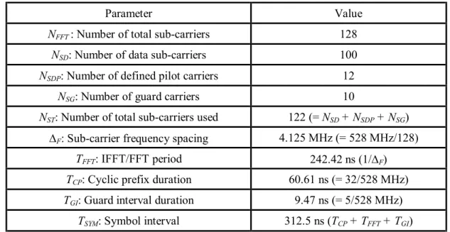
In Table 1.2, it lists timing-related parameters. An OFDM symbol period is
TSYM = TCP + TFFT + TGI = 312.5 ns. TCP is the cyclic prefix which is used in OFDM
to mitigate the effects of multi-path. The parameter TGI is the guard interval duration.
TFFT is the 128-point FFT period which is 242.42 ns.
Table 1.2 – Timing-related parameters for UWB
Parameter Value
NFFT : Number of total sub-carriers 128
NSD: Number of data sub-carriers 100
NSDP: Number of defined pilot carriers 12
NSG: Number of guard carriers 10
NST: Number of total sub-carriers used 122 (= NSD + NSDP + NSG)
DF: Sub-carrier frequency spacing 4.125 MHz (= 528 MHz/128)
TFFT: IFFT/FFT period 242.42 ns (1/DF)
TCP: Cyclic prefix duration 60.61 ns (= 32/528 MHz)
TGI: Guard interval duration 9.47 ns (= 5/528 MHz)
8
Fig. 1.6 shows the format for the PLCP frame. The PLCP frame includes PLCP preamble, PLCP header, frame payload, and inserted data. In PLCP preamble, 29 OFDM symbols are included. The packet synchronization sequences are used for packet detection and acquisition, coarse carrier frequency estimation, and coarse symbol timing. The frame synchronization sequences are used for synchronize the receiver algorithm. Finally, the channel estimation sequences {CE0, CE1, CE2, CE3, CE4, CE5} are used to estimate the channel frequency response, fine carrier frequency estimation, and fine symbol timing. In UWB specification, OFDM symbols are transmitted over three different sub-bands, so each sub-band can only use two channel estimation sequences.
9
1.4. Introduction to IEEE 802.16d Fixed WIMAX
WIMAX [3] is a standard-based wireless technology that provides high-throughput broadband connections over long distances. WIMAX can be used for a number of applications, including "last mile" broadband connections, hot spots and high-speed data transmission. The advantages of high spectral efficiency, Low cost of deployment and good cell coverage make WIMAX a great candidate for metropolitan area wireless communication.
1.4.1. Fixed-WIMAX physical layer
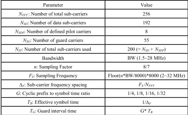
The block diagram of the fixed-WIMAX is similar to UWB. Except to the Convolutional Code, WIMAX system adds the Reed-Solomon Code. The IFFT/FFT point is 256. There are multiple choices of bandwidth, and the maximum bandwidth is 28Mhz. Some of important parameters are listed in Table 1.3 and Table 1.4.
Table 1.3 –Timing related parameters for WIMAX
Parameter Value
NFFT : Number of total sub-carriers 256
NSD: Number of data sub-carriers 192
NSDP: Number of defined pilot carriers 8
NSG: Number of guard carriers 55
NST: Number of total sub-carriers used 200 (= NSD + NSDP)
Bandwidth BW (1.5~28 MHz)
n: Sampling Factor 8/7
FS: Sampling Frequency Floor(n*BW/8000)*8000 (2~32 MHz)
DF: Sub-carrier frequency spacing FS /NFFT
G: Cyclic prefix to symbol time ratio 1/4, 1/8, 1/16, 1/32
TB: Effective symbol time 1/DF
10
Table 1.4 –Available bandwidth list for WIMAX
BW (MHz) TB (us) TG= TB/32 (us) TG = TB/16 (us) TG = TB/8 (us) TG= TB/4 (us) n=8/7 1.75 128 4 8 16 32 3.5 64 2 4 8 16 7.0 32 1 2 4 8 14.0 16 0.5 1 2 4 28.0 8 0.25 0.5 1 2
In fixed-WIMAX, there are seven different transmission types defined IEEE 802.16d standard. They are shown in Table 1.5.
Table 1.5 –Seven different transmission types for WIMAX
Modulation Uncoded block size (bytes)
Coded block size (bytes) Overall Coding rate RS code CC code rate BPSK 12 24 1/2 (12,12,0) 1/2 QPSK 24 48 1/2 (32,24,4) 2/3 QPSK 36 48 3/4 (40,36,2) 5/6 16-QAM 48 96 1/2 (64,48,8) 2/3 16-QAM 72 96 3/4 (80,72,4) 5/6 64-QAM 96 144 2/3 (108,96,6) 3/4 64-QAM 108 144 3/4 (120,108,6) 5/6
In IEEE 802.16d standard, the frame consists of a downlink sub-frame and an uplink sub-frame. With different duplexing methods, there are two frame structures. In this thesis, Frequency Division Duplex (FDD) is used to transmit the signal. Fig. 1.7 shows the FDD frame structure. The downlink PHY PDU starts with a long preamble. The preamble is followed by a FCH burst. FCH burst is one OFDM
11
symbol long and is transmitted using BPSK rate 1/2. It specifies burst profile and length of one or several downlink bursts immediately following the FCH. After FCH, data bursts are transmitted.
12
1.5. Channel Equalizer Design Spec
In OFDM system, the multi-path channel, AWGN, Carrier frequency Offset (CFO) between transmitter and receiver, and Sampling Clock Offset (SCO) between DAC and ADC, are the four main data distortion issues. In order to solve the multi-path channel effect, preambles are used to estimate the fading channel. Then, receiver uses the estimated channel to do the equalization. Because of the existence of AWGN, it will cause channel estimation (CE) error. This CE error will be propagated to the equalizer and leads to performance degradation. The way to lower down the CE error will be introduced in chapter 3.
Residual CFO and SCO will cause phase rotation in frequency domain, and result in ICI. Phase Error Tracker (PET) is applied in OFDM systems for phase rotation tracking and compensation. The detail algorithm for PET will also be introduced in chapter 3.
13
Chapter 2.
Design Specification of Dual-Mode
Channel Equalizer
2.1. Wireless Channel Model
In order to simulate the practical data transmission, the wireless channel model must be established. The channel model comprises multi-path fading channel, CFO, SCO, AWGN. The details are introduced individually below.
2.2. Intel Proposed UWB Multi-paths Channel Model
The Intel proposed channel model [4] is based on the observation that usually multi-path contributions generated by the same pulse arrive at the receiver grouped into clusters. The time of arrival of clusters is modeled as a Poisson arrival process with rate Λ: 1 ( ) 1
( |
n)
T Tn n np T T
e
(2.3)Where
T
n andT
n-1 are the times of arrival of the n-th and the (n-1)-th clusters. Within each cluster, subsequent multi-path contributions also arrive according to a Poisson process with rate λ:( 1) ( ) ( 1)
(
|
)
nk n k nk n kp
e
(2.4)14 within cluster k.
The channel impulse response of the IEEE model can be expressed as follow:
( ) 1 1 ( ) N K n nk ( n nk) n k h t X t T
(2.1)where X is a log-normal random variable representing the amplitude gain of the channel. N is the number of observed clusters. K(n) is the number of multi-path contributions received within the n-th cluster.
α
nk is the coefficient of the k-th multi-path contribution of the n-th cluster.T
n is the time of arrival of the n-th cluster, andτ
nk is the delay of the k-th multi-path contribution within the n-th cluster.The channel coefficient
α
nk can be defined as follows:nk
p
nk nk
(2.2)where
p
nk is discrete random variable assuming values ±1 with equal probability and βnk is the log-normal distributed channel coefficient of multi-path contributionk belonging to cluster n. Theβnk term can be expressed as follows:
20
10
xnk nk
(2.3)15 standard deviation
σ
nk .Variable
x
nk in particular, can be future decomposed as follows:n
nk nk nk
x
(2.4)where
ζ
n andξ
nk are two Gaussian random variables that represent the fluctations of the channel coefficient on each cluster and on each contribution. We indicate the variance ofζ
n andξ
nk by 2and 2. Theμ
nk value is determined to reproduce the exponential power decay for the amplitude of the multi-path contribution with in each cluster. One can write:
2 2 2 20 00 2 2 2 00 10 10ln 10 10 ln 10 ln 10 20 n nk nk nk Tn nk n n nk e e T (2.5)The total energy contained in the βnk terms must be normalized to unity for each realization, this is:
( ) 2 1 1 1 K n N nk n
k (2.6)The amplitude gain X in eq. 2.1 is assumed to be a log-normal random variable:
20
10g
16
Where
g
is Gaussian random variable with meang
0 and variance g2 . Theg
0 value depends on the average total multi-path gain G.2 0 10ln( )ln(10)G g ln(10)20
g (2.8)
The value can be determined as indicated below:
0 0 10 0 10 A G G D G (2.9)
In eq. 2.8, A0 (in dB) = 10log(ETX/ERX0). Values for both A0 and γ are
suggested in (Ghassemzadeh and Tarokh, 2003) for different propagation environments: A0=47dB and γ=1.7 for a LOS environment, and A0= 51dB and γ=3.5
for a NLOS environment.
According to the above definitions, the channel model represented by the impulse response is fully characterized when the following parameters are defined:
l Λ : The cluster average arrival rate l λ : The ray average arrival rate
l Γ : The power decay factor for clusters
l γ : The power decay factor for rays in a cluster
l s : The standard deviation of the fluctuations of the channel coefficients x
17
l s : The standard deviation of the fluctuations of the channel coefficients z
for rays in each cluster
l s : The standard deviation of the channel amplitude gain g
The IEEE suggested an initial set of values for the above parameters. These values will shows in Table 2.1.
Table 2.1 –Parameter Settings for the IEEE UWB Channel Model
Scenario Λ λ Γ γ s x s z s g Case A (CM1) LOS (0-4 m) 0.0233 2.5 7.1 4.3 3.3941 3.3941 3 Case B (CM2) NLOS (0-4 m) 0.4 0.5 5.5 6.7 3.3941 3.3941 3 Case C (CM3) NLOS (4-10 m) 0.0667 2.1 14 7.9 3.3941 3.3941 3 Case D (CM4)
Extreme NLOS Multi-path Channel
0.0667 2.1 24 12 3.3941 3.3941 3
The channel impulse response (CIR) and the corresponding channel frequency response (CFR) of CM2, CM4 are shown in Fig. 2.1.
18
19
2.3. WIMAX SUI Channel Model
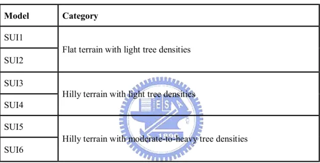
In 802.16d system, a series of Stanford University Interim (SUI) [5] channel with three terrain types are selected for application on fixed broadband wireless. According to the different terrain and tree density, the six SUI channels can be classified into three categories as showed in Table 2.2
Table 2.2 –SUI Channel
Model Category
SUI1
Flat terrain with light tree densities SUI2
SUI3
Hilly terrain with light tree densities SUI4
SUI5
Hilly terrain with moderate-to-heavy tree densities SUI6
The narrow band received signal fading can be characterized by a Ricean distribution. The key parameter of this distribution is the K-factor, defined as the ratio of the “fixed” component power and the “scatter” component power. The narowband K-factor distribution was found to be lognormal, with the median as a simple function of season, antenna height, antenna beamwidth, and distance. The standard deviation was found to be approximately 8 dB. K-factor model is presented as follows:
0 S h b
20
Where
F
S is a seasonal factor,F
S =1.0 in summer (leaves):2.5 in winter (no leaves)F
h is the receive antenna height factor,Fh =( /3)h 0.46(h
is the receive antennaheigh in meters)
F
b is the beamwidth factor,F
b=
( /17)
b
-0.62 (b
in degrees)K
0 andγ
are regression coefficients,K
0= 10;γ
= -0.5u
is a lognormal variable which has zero dB mean and standard deviation of 8.0 dB We use the method of filtered noise to generate channel coefficients with the specified distribution and spectral power density. For each tap a set of complex zero-mean Gaussian distributed numbers is generated with a variance of 0.5 for the real and imaginary part. Total average power of this distribution is 1. This yields a normalized Rayleigh distribution for the magnitude of the complex coefficients. For the Ricean distribution (K>0), a constant path component m has to be added to the Rayleigh set of coefficients. The ratio of powers between this constant part and the Rayleigh (variable) part is specified by the K-factor. The following equation shows the distribution of the power by stating the total powerp
of each tap.2 2 2 2 2 1 2 1 1 P m m K K P and m P K K (2.11)
Where m is the complex constant and 2 is the variance of the complex Gaussian set. The generated coefficients of channel taps have a white spectrum since they are independent of each other. The SUI channel model defines a specific power spectral
21
density (PSD) function for these scatter component channel coefficients is given as:
ì - + £ ï = í = > ïî 2 4 0 0 0 0 0 1 1.72 0.785 , 1 ( ) 0 , 1 m f f f f S f where f f f (2.12)
To arrive at a set of channel coefficients with this PSD function, we correlate the original coefficients with a filter which amplitude frequency response is derived from eq. 2.12 as
=
( ) ( )
H f S f (2.13)
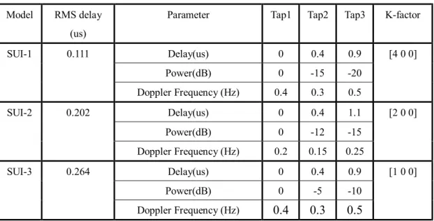
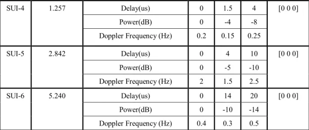
Without changing the total power of transmitted signal, the total power of the Doppler filter has to be normalized to one. Consequently, after passing through the Doppler filter, normalized factor is applied to normalize these multi-path fading taps. Table 2.3 shows the parameters of six SUI channels. Table 2.4 shows the normalization factor for each SUI channel.
Table 2.3 -SUI Channel Parameters
Model RMS delay (us)
Parameter Tap1 Tap2 Tap3 K-factor
SUI-1 0.111 Delay(us) 0 0.4 0.9 [4 0 0] Power(dB) 0 -15 -20 Doppler Frequency (Hz) 0.4 0.3 0.5 SUI-2 0.202 Delay(us) 0 0.4 1.1 [2 0 0] Power(dB) 0 -12 -15 Doppler Frequency (Hz) 0.2 0.15 0.25 SUI-3 0.264 Delay(us) 0 0.4 0.9 [1 0 0] Power(dB) 0 -5 -10 Doppler Frequency (Hz) 0.4 0.3 0.5
22 SUI-4 1.257 Delay(us) 0 1.5 4 [0 0 0] Power(dB) 0 -4 -8 Doppler Frequency (Hz) 0.2 0.15 0.25 SUI-5 2.842 Delay(us) 0 4 10 [0 0 0] Power(dB) 0 -5 -10 Doppler Frequency (Hz) 2 1.5 2.5 SUI-6 5.240 Delay(us) 0 14 20 [0 0 0] Power(dB) 0 -10 -14 Doppler Frequency (Hz) 0.4 0.3 0.5
Table 2.4 -Normalization Factors
SUI Channel Models Normalization Factor (dB)
SUI-1 -0.1771 SUI-2 -0.3930 SUI-3 -1.5113 SUI-4 -1.9218 SUI-5 -1.5113 SUI-6 -0.5683
For system bandwidth equal to 20MHz, the examples of CIR and CFR for SUI-1 to SUI-3 are shown in Fig. 2.2 to Fig. 2.4.
23
Fig. 2.3 CIR and CFR for SUI-2
24
2.4. Carrier Frequency Offset Model
Carrier Frequency Offset (CFO) [1] is caused by the mismatch in RF local frequency between transmitter and receiver. When CFO is existed in transmission path, the received sub-carrier will be influence by the other sub-carriers, which is referred as ICI. ICI effect caused by CFO is shown in Fig. 2.5.
-5 -4 -3 -2 -1 0 1 2 3 4 5 -0.4 -0.2 0 0.2 0.4 0.6 0.8 1 -5 -4 -3 -2 -1 0 1 2 3 4 5 -0.4 -0.2 0 0.2 0.4 0.6 0.8 1 1 f f2 f3 f4 f5 fD 1 f +fD f2+ fD
Fig. 2.5 ICI effect
Assuming the transmitted signal is S(t), transmitted carrier frequency is
f
c , received carrier frequency is fc f ,
f
is the sub-carrier spacing, and
is the frequency offset. The received signal after down conversion is given as:2 2 ( ) 2
( )
( ) e
j f tce
j fc f t( ) e
j f tR t
S t
S t
(2.12)Finally, CFO effect is simulated by multiplying the original signal with a phase rotation. This phase rotation is increased by the time as it can be seen from eq. 2.12.
25
2.5. Sampling Clock Offset Model
SCO is caused by ADC/DAC sampling frequency mismatch. Because of SCO, the sampling points will slowly shift with time. This shift in time domain will result in phase rotation in frequency domain and ICI. Fig. 2.6 shows the concept of SCO, where
T
s is the sampling time andμ
is the value of timing offset.m + 1 ( ) S T S T
Fig. 2.6 SCO effect
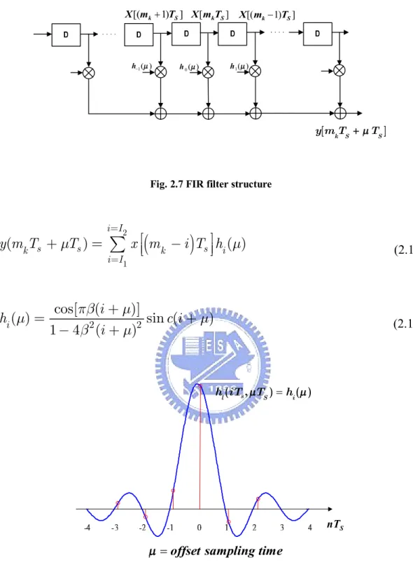
The SCO model is established by the concept of interpolation with 20 taps raised cosine filter [6]. The FIR filter structure of the interpolator is shown in Fig. 2.7. This filter performs a linear combination of (I1+I2+1=20) signal samples
x(nT
S)
taken around the basepointm
k , and the operation can be shown in eq. 2.13. In eq. 2.13,h
i( )
is the coefficient of FIR filter tap, the sampled value of the raised cosine function. The corresponding sampled value is shown in eq. 2.14 and Fig. 2.8.26 1( ) h- m h0( )m h1( )m [( k 1) ]S X m + T X m T[ k S] X m[( k-1) ]TS m [ k S S] y m T + T
Fig. 2.7 FIR filter structure
2 1(
k s s)
i I k s i( )
i Iy m T
T
x m
i T h
(2.13) 2 2cos[ (
)]
( )
sin (
)
1 4 (
)
ii
h
c i
i
(2.14) m = m ( ,s ) ( ) l S i h iT T h S nT offset sampling timem =
27
2.6. Additive White Gaussian Noise
The AWGN is established by the random generator (randn). The output random signal is normally distributed with zero mean and variance equal to 1. The AWGN noise can be modeled as
10
10
[
(1, )
(1, )]
2
S P SNRw
randn n
j randn n
(2.15)Where PS is signal power, SNR is signal-to-noise ratio (dB), and n is length of data signal.
28
Chapter 3.
Design of Dual-Mode Channel
Equalizer
In this chapter, a low complexity and high performance dual-mode channel equalizer is proposed. It includes channel estimator, equalizer, phase error tracker and modified normalized least-mean-square (NLMS) channel tracker. Data distortion caused by multi-path fading, AWGN, residual CFO and SCO can be eliminated by these four parts. Following is the block diagram of the proposed channel equalizer. After passing through the FFT, channel estimator uses received preambles to estimate the channel frequency response (CFR). The estimated CFR will be sent to the equalizer. Then, equalizer uses the estimated CFR to equalize the distorted data sub-carriers. After doing the equalization, equalized data sub-carriers will be sent to the phase error tracker and compensator. The tracked phase error combined with unequalized data, equalized data and estimated CFR are then sent to modified NLMS channel tracker to calculate the updated CFR. Finally, compensated data sub-carriers are sent to De-Mapper.
29
3.1. Dual-Mode Design of Channel Estimation
The signal is transmitted over frequency-selective fading channel. After removing the cyclic prefix and guard interval, the post-FFT signal of the l-th OFDM symbol can be expressed by:
p 1 2 ( / ) , 0 ( ) N j n N k l l n n Y k z e
(3.1)where
z
l n, is the time domain data, N is the number of FFT points. Under consideration of CFO Df , SCOz =( 'T T T- ) / , and symbol timing offsetn
e , thepost-FFT signal can be simplified as an equivalent model [7]:
e p f p e
a f a
+ = × + [ 2 ( )/ ] [ 2 ( / ) ] , ( ) ( ) ( ) ( ) j k N n j l k T Tu g Tu l k l k l k Y k n X k H e e W (3.2)wherefk = DfTu + ×z k ,a( ), ( )ne a fk are the attenuation factors,X kl( )is the
transmitted data at the k-th sub-carrier,
T
uis the duration of FFT,T
g is the guardinterval,
T
is the sampling time,T
'
is the offset sampling time, W is the noise ,lk caused by AWGN, symbol timing offset, ICI, and other non-ideal parameters. With the assumption that the timing synchronization is perfect, there is no timing offset. The equivalent model can be simplified as:p f a f + = [ 2 ( )/ ] + , ( ) ( ) ( ) j l k T Tu g Tu l k l k l k Y k X k H e W (3.3)
30
3.1.1. Channel Estimation for UWB
In UWB system, use zero-forcing (ZF) methodology with received two preambles to estimate the fading channel. Using the average value, the estimation error can be reduced and the performance will be improved. Simulation result shows that it will contribute 1~2dB gain in SNR. Considering that the pre-defined signal
( )
L
X k in preamble, the estimated of the k-th sub-channel is given by:
1 2
( ) ( ) ( ) / 2 ( )
E L L L
H k Y k Y k X k (3.4)
Where
Y
L1( )
k
,Y
L2( )
k
are the first and second received preamble.In channel estimation, these two received preambles are also used to estimate the noise power which can be described as follows:
1 2 1 2 2 1 2 0 0 1 2 2 1 2 0 1 1 ( ) ( ) ( ) 2 1 ( ) ( ) 2 N N L L E k k N E L L k Y k Y k W k N N Y k Y k N s s - -= = -= - » » ® =
-å
å
å
V (3.5)Where ΔW(k) is the white noise,
s
2E is the estimated noise power.Based on the correlative property between adjacent sub-channels, the estimation of sub-channels can be further improved by delivering them into the 3-taps smoothing filter. The smoothing filter is a finite impulse response filter [8], which can be described as:
d =-× -=
å
å
1 1 1 1 ( ) ( ) m m m m c k m S k c (3.6)31
After doing channel estimation, the estimated sub-channel H k will be E( ) convoluted by the smoothing filter. The equation is given by:
=-=
å
1 - × 1 ( ) ( ) ( ) S E m H k H k m S m (3.7)After smoothing, each sub-channel will be a weighted summation of itself and nearby sub-channels. Simulation reveals that the system performance on PER will improve about 1dB for different transmission modes.
3.1.2. Channel Estimation for WIMAX
In WIMAX system, long preamble is used to estimate the fading channel. In standard of 802.16-2004, only even sub-carriers are utilized in long preamble. DC sub-carrier and odd sub-carriers are transmitted with zero value. Consequently, the ZF methodology is used to estimate the CFR of even sub-carriers at first, and then use 6-tap raised-cosine interpolator to get CFR of DC sub-carrier and odd sub-carriers. Following is the description of channel estimation for WIMAX system.
Considering that the pre-defined signalX k in preamble, the estimated CFR L( )
of the k-th even sub-carrier is given by:
, ( ) ( ) / ( )
E even L L
H k Y k X k (3.8)
Where
Y
L(k)
is the received long preamble.Then, the 6-tap raised-cosine interpolator [6] is used to interpolate the CFR of odd sub-carriers and DC sub-carrier. Following is the impulse response of 6-tap
32 raised-cosine interpolator: 2 2 2 sin( / ) cos( / ) ( ) / 1 4 / k D k D W k k D k D (3.9)
Where D is the spacing of even sub-carriers, and β is the roll-off factor. And, let k equal to -5, -3, -1, 1, 3, 5, the coefficient of six taps can be generated.
But, using 6-tap raised-cosine interpolator to get CFR of sub-carrier number -99, -97, 97, 99 will result in large error [9]. For example, to get CFR of sub-carrier number -99, it needs CFR of sub-carrier number -104, -102, -100, -98, -96, -94. But, sub-carriers are transmitted with zero value at number -104, -102. Receiver doesn’t have any information at these two places. If zero value is applied to substitute the CFR of these two places, it will result in large error. So, the linear interpolation is used to get the CFR of sub-carrier number -99, -97, 97, 99.
Otherwise, DC sub-carrier (number 0) is transmitted with zero value. In order to get CFR of sub-carrier number -5, -3, -1, 1, 3, 5, CFR of DC sub-carrier is needed. To interpolate the DC value, CFR of sub-carrier number -10, -6, -2, 2, 6, 10 are used to get the CFR of DC sub-carrier [9]. Next, DC value is used to get the CFR of sub-carrier number -5, -3, -1, 1, 3, 5. For example, to interpolate the CFR of sub-carrier number 5, CFR of sub-carrier number DC, 2, 4, 6, 8, 10 are used as inputs to the interpolator. Following the same rule, CFR of sub-carrier number -5, -3, -1, 1, 3 can be generated.
According to the above statement, 6-tap raised-cosine interpolator is needed. Using 6-tap raised-cosine interpolator to get CFR of odd sub-carrier can be described as follows:
33 2 2 2 , 1 3 sin( ( 1)/ ) cos( ( 1)/ ) ( ) . ( 1)/ 1 4 (( 1)/ ) E odd k mD m mD D mD D H k H mD D mD D
(3.10)Using ZF channel estimation with 6-tap raised-cosine interpolator, the whole CFR can be generated.
3.2. Dual-Mode Design of Equalization
For UWB system, the modulation type is QPSK. Minimum mean square error (MMSE) methodology is very suitable to equalize the distorted signal. Traditional zero-forcing equalization will increase the noise and degrade the system’s performance. Consequently, MMSE equalization is used to suppress the interference and noise effects in UWB system. The compensating value of the MMSE equalization can be derived as:
s = + * 2 2 2 ( ) ( ) ( ) ( ) S MMSE E S L H k C k H k X k (3.11)
Where
H
s(k)
is the smoothed CFR, and s2E is estimated noise power from
channel estimation part, X kL( )2is transmitted preamble power, which can be fixed as 1 in UWB system. Finally, the signal is equalized as:
ˆ ( )l l( ) MMSE( )
X k =Y k C× k (3.12)
For WIMAX system, there are four different modulation types, such as BPSK, QPSK, 16-QAM, 64-QAM. For 16-QAM, 64-QAM conditions, using MMSE
34
methodology to do equalization will suppress the signal and noise simultaneously. The attenuation signal will cross the decision boundary, and result in decision error. Consequently, MMSE methodology is not suitable for WIMAX system. In this place, ZF methodology is used to equalize the distorted signal. Following is the compensating value of the ZF equalization:
( ) 1/ ( )
ZF E
C k H k (3.13)
Next, the signal is equalized as:
ˆ ( )l l( ) ZF( )
X k =Y k C× k (3.14)
3.3. Dual-Mode Design of Phase Error Tracking and compensation
CFO and SCO are the other two data distortion sources for OFDM systems, which are caused mainly by a crystal oscillator frequency mismatch between transceiver and DAC/ADC mismatch. Generally, timing synchronization is applied to compensate these two effects. Nevertheless, other impairments will make the synchronization imperfect. The residual CFO and SCO will cause the data phase rotation in frequency domain and result in inter-carrier interference (ICI). In case of a coherent demodulation scheme, the error due to the rotation of a signal constellation will be fatal for transmission bursts, because the accumulated phase rotation will shift the constellation point to cross the decision boundary. It will cause high error rates and therefore the phase error tracking (PET) is applied in OFDM systems for phase rotation tracking and compensation.35 simplified as: p f
a
+=
' [ 2 ( )/ ]+
',( )
( )
j l k T Tu g Tu l l l kY k
X k e
W
(3.15)Where a is attenuation factor, and ' W is AWGN noise and another non-ideal l k',
effect. The phase rotation of the l-th symbol and k-th sub-carrier can be derived as:
p pz æ + ö Ð = D + + çç ÷÷ è ø ˆ ( ) 2l ( u g) 2 u g g T T X k l f T T lk T (3.16)
The first term is caused by CFO effect. This phase rotation is constant for all data sub-carriers in an OFDM symbol and increases with symbol index. The second term is caused by SCO effect, which is a linear phase rotation with sub-carrier index. This also increases with symbol index. So, the PET is used to track the mean phase error caused and phase error slope caused by these two effects.
The PET is designed based on the known pilot sub-carriers. In order to achieve correct tracking of phase error exceeding ±p , the pre-compensation [10] is added in the PET. Before PET, the pilot sub-carriers will first be compensated with the phase error tracked in the previous OFDM symbols. Therefore, only the difference of the phase error between previous and preset OFDM symbols needs to be tracked with pilot sub-carriers. This will enhance the PET accuracy. The PET algorithm with pre-compensation is given as:
36 { } { } as otherwise q q q j - g -Î - - - -Î - - - -= ì ü ï ï D = í ý - - × ï ï î þ , , , 1 1 5,15, 25, 35, 45, 55, 5, 15, 25, 35, 45, 55 13, 38, 63, 88, 13, 38, 63, 88 1 l K l K l K l l UWB WIMAX K K l K (3.17)
Where K is the pilot index list, for UWB system, K=KUWB , for WIMAX system,
K=KWIMAX , l=1 means the first received OFDM symbol, ,lK is the detected phase
error of l-th OFDM symbol,
,lK is defined as the pilot phase after pre-compensation with the previous tracked phase error l1 K l1.Next, use the pre-compensation pilot phase to calculate the mean phase error
l
, which can be shown in eq. 3.18 and phase error slope
g
l, which can be shownin eq. 3.19, and the related parameters for UWB and WIMAX systems are shown in eq. 3.20. as otherwise q j q j -ì D = ü ï ï ï ï = í ý ï D + ï ï ï î þ
å
å
, , 1 1 1 1 l K K l l K l K l p p (3.18)where p is the number of pilot sub-carriers, jl-1 is previous tracked mean phase
error. as otherwise g q q g q q g + -+ -D - D ì ü ï = ï ï ï = í D - D ý ï ï ï + ï î þ
å
å
å
å
, , , , 1 1 l K l K K K l l K l K K K l l C W C (3.19)37
where gl-1is the previous, Wg , C are constant terms, K+ is index list of positive
pilot sub-carriers , K- is index list of negative pilot sub-carriers.
{
}
{
}
{
}
{
}
5,15, 25, 35, 45, 55 13, 38, 63, 88 5, 15, 25, 35, 45, 55 13, 38, 63, 88 360 12 404 8 UWB WIMAX UWB WIMAX K K K K C p for UWB C p for WIMAX + + - -= = = - - - = - - - -= = = = (3.20)To consider the hardware complexity, the proposed phase error tracker has the advantage of reducing the multiplicative computation. In the pilot phase pre-compensation part, it only needs one multiplier. Using mean-average method, it only needs to do constant multiplication of two times in each OFDM symbol.
After PET, the data sub-carriers are compensated according to the tracked phase error, which can be indicated as:
ˆ
( ) ( ) exp( ( ))
l l l l
X k% = X k × -j j +kg (3.21)
According to Fig. 3.1, after doing compensation, the data X k%l( )is sent to the De-Mapper.
3.4. Modified-NLMS Channel Tracking
In WIMAX system, only even sub-carriers are utilized in long preamble. Consequently, interpolator is used to get the CFR of odd sub-carriers. Because the ideal interpolator is not practical, there is some aliasing effect occurred in interpolation. Aliasing effect will increase the channel estimation error, and degrade
38
the performance of equalizer. Otherwise, noise, interference and time-variant characteristic will also increase the channel estimation error. Consequently, channel tracker is applied to mitigate the above non-ideal effects and enhance the accuracy of channel estimation.
Standard LMS methodology suffers from a gradient noise amplification problem. To overcome this difficulty, NLMS methodology normalizes the adjustment of tap-weight vector. But, in OFDM system, residual CFO and SCO will result in phase rotation in frequency domain. The traditional NLMS methodology can not be directly used. So, the modified-NLMS methodology is proposed with consideration the phase rotation. Following is the detail algorithm of proposed modified-NLMS channel tracking.
The equalized signal after compensating with tracked phase error is sent into slicer (map the signal to nearest constellation point according to modulation type) to compute the decision signalX kl( ). For each sub-carrier k, a single tap frequency domain NLMS filter is used. The modified-NLMS error E k is as follows: l( )
1
( ) ( ) exp( ( ) ( ) l ( )
l l l l l
E k Y k j k X k H k (3.22)
Where Y kl( ) is unequalized signal of l-th OFDM symbol, l kl is the compensated phase error com from PET, Hl1( )k is the previous estimated CFR.
39 * 2 ( ) ( ) ( ) ( ) l l l l X k H k E k X k (3.23)
Finally, using the gradient and previous estimated CFR, the update eq is given as:
1
( ) ( ) ( )
l l l
H k H k H k (3.24)
Where is the constant gain.
Then, the updated CFR H kl( )can be used for next OFDM symbol.
40
Chapter 4.
Simulation Result and Performance
Analysis
In order to verify the proposed design, complete system platforms are established according to the UWB standard (802.15.3a) and the fixed WIMAX standard (802.16d) on Matlab. The platform has been introduced in chapter 1. Channel estimation accuracy, PET performance, and system performance will be simulated and compare to system constraint of two standards.
4.1. Performance Analysis of the Proposed Dual-Mode Channel
Equalizer for UWB system
To analyze the performance of a proposed scheme, we simulate the PER (%) for different SNR and different CFO, SCO value with CFO and SCO variation being considered. The simulation is processed with multi-paths CM2 channel with data rate 480 (Mb/s). The simulation result is shown in Fig. 4.1. The cross-section view for PER (%) with different CFO, SCO values is shown in Fig. 4.2. From the simulation result, it shows that the proposed PET can track the phase error correctly and compensate the phase error under 60 ppm of CFO, SCO value. Above 60 ppm of CFO, SCO value, resulted ICI and phase error will increase grossly to degrade the system performance. Under IEEE 802.15.3a demanded [2], the CFO, SCO value should be less than total 40 ppm (±20 ppm), and the proposed PET can track the phase error accurately.
41
Fig. 4.1 PER (%) simulation for different SNR and CFO, SCO value under CM2, data rate 480Mb/s 0 10 20 30 40 50 60 70 80 90 100 0 10 20 30 40 50 60 70 80 90 100 CFO,SCO (ppm) PE R (%) CM2, SNR=17, Data rate=480Mbit/s
Fig. 4.2 PER (%) simulation result with different CFO, SCO value in CM2
In most WLAN and WPAN systems, a PER less than 8% is required. Therefore, PER 8% can be the indication of system performance. The PER (%) with different transmission mode and different channel model are shown in Fig. 4.3. and Fig. 4.4. Simulation results show that for channel model CM4, data rate 110Mbit/s, with the requirement of 8% PER, the proposed design can achieve this demand at SNR 6.98dB. For transmission in AWGN, the proposed scheme can get this demand at
42
SNR 2.82dB. The comparison of simulation results with system constraint and references is shown in Table 4.1. It shows that the proposed design can achieve 1.36dB to 7.25dB gain in SNR for different simulation conditions.
0 2 4 6 8 10 12 10-1 100 101 102 SNR(dB) PE R (%) AWGN,Data rate=480Mbit/s AWGN,Data rate=200Mbit/s AWGN,Data rate=110Mbit/s 8%
Fig. 4.3 PER (%) simulation result for different data rates in AWGN channel with 40 ppm of CFO, SCO value
2 4 6 8 10 12 14 16 18 20 22 24 10-1 100 101 102 SNR(dB) PE R (%) CM2,Data rate=480Mbit/s CM4,Data rate=200Mbit/s CM4,Data rate=110Mbit/s 8%
Fig. 4.4 PER (%) simulation result for different data rates and channel model with 40 ppm of CFO, SCO value
43
Table 4.1 –Performance Result for UWB system
Entry Proposed [11] [12] System
Constraint AWGN Data rate=200Mbits/s 3.8 dB 3.8 dB 4.11 dB 5.16 dB AWGN Data rate=480Mbits/s 6.65 dB 7.2 dB 5.03 dB 9.66 dB CM4 Channel &AWGN Data rate=200Mbits/s 9.91 dB 14.2 dB 14.18 dB 15.1 dB CM2 Channel &AWGN Data rate=480Mbits/s 13.85 dB 18.5 dB 15.01 dB 21.1 dB
It should be noted that under the worst environment, CM4, the proposed dual-mode channel equalizer will have 5.19dB gain. In the case of receiving data rate of 480Mbit/s, it will have 7.25dB gain. Hence, the proposed joint scheme makes the receiver more robust to CFO and SCO effects and could suppress the error rate at low SNR with high data rate receiving.
44
4.2. Performance Analysis of the Proposed Dual-Mode Channel
Equalizer for WIMAX system
In WIMAX system, the accuracy of channel estimation is a key factor for system performance. To analyze the accuracy of channel estimation, mean-square-error (MSE) between estimated CFR and real CFR is measured. Performance of proposed modified-NLMS channel tracker is simulated with condition under SUI-3 channel, 64-QAM modulation. Following is the comparison of MSE between using modified-NLMS channel tracker and without modified-NLMS channel tracker.
Fig. 4.5 MSE analysis of Modified-NLMS channel tracker
The proposed modified-NLMS channel tracker contributes 3~18dB gain in MSE compared with only ZF channel estimation. Fig. 4.6 shows the channel estimation error from sub-carrier number 70 to sub-carrier number 110, between ideal CFR, using modified-NLMS channel tracker and without modified-NLMS channel tracker.
45
Fig. 4.6 Channel Estimation Error from sub-carrier number 70 to 110
The rate of convergence of modified-NLMS channel tracker depends on the step size. Smaller step size will converge much slower than larger step size. But, smaller step size will contribute smaller MSE than larger step size. Following is the learning curve of proposed modified-NLMS channel tracker with 300 iterations. In this simulation, we select step size with the value equal to 0.0085.
46
Fig. 4.8 shows the bit error rate (BER) with modified-NLMS channel tracker and without modified-NLMS channel tracker under SUI-3 channel, 64-QAM modulation, CFO=0.1 ppm, SCO=16 ppm.
Fig. 4.8 BER Comparison
As it can be seen from Fig. 4.8, design with proposed modified-NLMS channel tracker can contribute 1 dB SNR gain than design without modified-NLMS channel tracker. And, by using modified-NLMS channel tracker, it only result 1 dB SNR loss comparing to use ideal channel. Under different simulation conditions, modified-NLMS channel tracker can contribute different SNR gain. From simulation results, modified-NLMS channel tracker can contribute 1~1.5 dB SNR gain with different simulation conditions.
In 802.16d standard, CFO, SCO value should less than ±8 ppm. With the aid of synchronization, we assume the residual CFO is 0.1 ppm. The BER curves of different transmission mode under SUI-1 to SUI-3 channel, system bandwidth=20MHz, CFO=0.1 ppm, SCO=16 ppm are shown in Fig. 4.9, Fig. 4.10, and Fig. 4.11. Table 4.2 shows the required SNR to attain 10^-6 BER under SUI-3
47
Fig. 4.9 BER performance under Bandwidth=20 MHz, CFO=0.1 ppm, SCO=16 ppm, SUI-1 channel
Fig. 4.10 BER performance under Bandwidth=20 MHz, CFO=0.1 ppm, SCO=16 ppm, SUI-2 channel