長期演進技術中非連續接收機制之服務品質與省電效能分析

(1)

國立交通大學

電信工程研究所

碩士論文

長期演進技術中非連續接收機制之服務品

質與省電效能分析

Quality of Service and Power Saving Analysis of DRX

Mechanism in LTE-Advanced Networks

研究生：吳咨翰

指導教授：李程輝教授

(2)

長期演進技術中非連續接收機制之服務品質與省電效能分析

Quality of Service and Power Saving Analysis of DRX Mechanism in

LTE-Advanced Networks

研究生：吳咨翰 Student：Tzu-Han Wu

指導教授：李程輝 Advisor：Tsern-Huei Lee

國立交通大學

電信工程研究所

碩士論文

A Thesis

Submitted to Institute of Communications Engineering College of Electrical and Computer Engineering

National Chiao Tung University in partial Fulfillment of the Requirements

for the Degree of Master in

Communications Engineering July 2013

Hsinchu, Taiwan, Republic of China

(3)

長期演進技術中非連續接收機制

之服務品質與省電效能分析

學生：吳咨翰

指導教授：李程輝博士

國立交通大學電信工程研究所碩士班

摘要

隨著越來越快速的無線通訊及智慧型手機的普及，用戶端設備如何達

到省電功效是一項亟需研究的課題。為了提高用戶設備於資料傳輸中的省

電效能，進階長程演進計畫在標準中訂定一項非連續接收機制，透過此機

制可減少不必要的電力消耗，然而降低電力消耗與維持服務品質是一體兩

面，本研究將探討非連續接收機制電力消耗與封包遺失狀況的關係。過去

探討非連續接收機制省電效能的研究，都僅以平均封包延遲時間做為服務

品質的衡量標準。本次研究在給定非連續接收機制參數設定值的情況下，

推導出封包遺失機率及用戶省電效能的計算式。由於目前尚未有通用的非

連續機收機制參數設定方式，本次研究也提出一套設定參數的方法。設定

的概念為在不違反服務品質要求下，選擇能盡量增加省電效率的參數組合。

研究所提出的數學計算式與參數設定方式都分別與電腦模擬與最佳參數設

定做比較。比較結果顯示由數學式求得的封包遺失機率及省電效能與電腦

模擬結果相符，本次研究提出的參數設定在不違反服務品質要求下，所對

應的省電效率也與最佳參數設定的省電效能相差不多。

關鍵字：非連續接收機制、省電機制、服務品質

(4)

ii

Quality of Service and Power Saving Analysis of DRX

Mechanism in LTE-Advanced Networks

Student: Tzu-Han Wu

Advisor: Dr. Tsern-Huei Lee

Institute of Communications Engineering

National Chiao Tung University

ABSTRACT

With demand for better user experience, performance of power saving on mobile phones has been a critical issue in recent years. In LTE-Advanced network, a Discontinuous Reception (DRX) mechanism is provided to support power saving functionality. It is clear that there is a trade-off between energy saving and quality of service (QoS). Unlike previous studies, which analyzed the average packet delay as QoS requirement, an analytical model for ratio of packet loss due to violation of delay bound requirement is proposed in this work and given DRX parameter values, equations for power consumption are also derived. Under the constraint that the packet loss ratio is no greater than a pre-defined threshold, an approach to maximizing average power saving is presented for selection of values for DRX parameters. The analytical model is verified with computer simulation and the result of analytical calculation matches that of simulation. Moreover, the power saving efficiency achieved by the proposed approach is close to that of optimum configuration. This work is expected to provide a fundamental analysis for packet loss probability and power saving efficiency under DRX mechanism.

(5)

誌謝

感謝指導教授李程輝老師在我就讀碩士班期間，無論是在平時討論

或是實驗室團體報告時，都能針對我在研究上所遇到的問題提出解決的方

法，以及建議我未來研究的方向。從老師身上我學到了對研究學問應該有

的態度和對人處事的價值觀，在老師的指導下，學生可以很自由地選擇自

己想研究的方向及內容，很幸運當初入學時能進入李老師實驗室，讓我的

碩士生活過得非常充實，也在這段期間吸收了很多。

感謝一起做研究、做計劃的承潔學姊，在完成研究的路上幫忙了非常

多，像一位模範一樣讓人有可以學習的榜樣。除了老師之外，承潔學姊也

給了我很多實質的建議，也常幫助我突破自己在研究上的瓶頸與盲點。

感謝實驗室的所有夥伴，梓洋學長、裕捷、瑞良、嘉振、鐙標、俊緯、

廣煜、彥良、廷勇、政谷、宗翰，平時一起討論、一起聊天、一起玩樂，

讓我覺得身為工四 823 實驗室這個大家庭的一份子是一件很驕傲的事。

感謝我的父親、母親及所有家人，支持我及鼓勵我，讓我在求學生涯

能沒有後顧之憂地完成學業。

最後再一次感謝各位，能讓我順利完成這篇論文，謹將此論文獻給身

邊所有陪伴我的人。

(6)

 

₁ 2.3.2 Derivation of E M

 

2 ... 14

2.3.3 Derivation of E M

 

₃ ... 15

2.3.4 Derivation of E N

 

... 16

2.4 Analysis of Power Saving Efficiency ... 17

2.4.1 Derivation of E T

 

A ... 17

(7)

2.4.3 Derivation of E T_ _{S on}_{_} _ ... 20

Chapter 3 QoS Support ... 22

3.1 Proposed DRX Parameters Configuration ... 22

Chapter 4 Verification ... 26

4.1 Verification of Numerical Analysis ... 26

4.2 Verification of Proposed Configuration ... 31

Chapter 5 Conclusion ... 33

References ... 34

(8)

List of Figures

Figure 1 DRX cycle ... 4 Figure 2 Example of DRX mechanism ... 4 Figure 3 Example of super cycle ... 7 Figure 4 Impact of Inactivity Timer on power saving efficiency and packet loss

probabilty for 0.1, Ton2 ms , CL256ms , CS 16ms , NSC 2

with D100ms. ... 23 Figure 5 Impact of Long Cycle Length on power saving efficiency and packet loss

probabilty for 0.1, T_on 2ms, C_T 1ms, C_S 16ms, N_SC 2 with 100

D ms. ... 24 Figure 6 Packet loss probabilty and power saving efficiency with different Long Cycle

Lengths for 0.01, 0.1 , T_on 2ms, C_T 10ms, C_S 16ms, N_SC 2, 150

D ms. ... 27 Figure 7 Packet loss probabilty and power saving efficiency with different Short Cycle

Lengths for0.01, 0.1 , T_on 2ms, C_L 512ms, C_T 10ms, N_SC 2, 150

D ms. ... 28 Figure 8 Packet loss probabilty and power saving efficiency with different Short Cycle

Timers for  0.01, 0.1 , T_on 2ms , C_L 512ms , C_S 16ms , 10

T

C  ms,D150ms. ... 29 Figure 9 Packet loss probabilty and power saving efficiency with different Inactivity

Timers for0.01, 0.1 , T_on2ms, C_L 512ms, C_S 16ms , N_SC 2, 150

D ms. ... 30 Figure 10 Performance comparison between proposed DRX configuration and optimum

(9)

List of Tables

(10)

Notations

Notation Definition on T On Duration T C Inactivity Timer L

C Long Cycle Length

S

C Short Cycle Length

SC

N Short Cycle Timer

 Arrival rate of Poisson process

p _{Packet loss ratio}

e Power saving efficiency

 _{Threshold of packet loss probability}

g _{Probability of having one packet arrival in one millisecond}

k

s , l , _k d _k Probability of having k packet arrivals in time interval of CS

_,

L

C  and D , respectively

S

C  Length from the ( )

th on

T sub-frame of On Duration to the end of current DRX Short Cycle

L

C  Length from the ( )

th on

T sub-frame of On Duration to the end of current DRX Long Cycle

D Delay Bound

(11)

G Probability of having packet arrival(s) in (Ton 1) sub-frames

N Number of dropped packets in a super cycle

K Number of buffered packets right before an exceptional first busy

period

1

M Number of packet arrivals in an exceptional first busy period

2

M Number of packet arrivals in busy periods of a super cycle

3

M Number of packet arrivals in a sleeping state

_

S on

T Length of UE power on in a sleeping state

S

T Length of a sleeping state

A

(12)

Chapter 1 Introduction

1.1 Enhancements on Diverse Data Applications

With the development of faster and cheaper mobile networks, more and more smart phones are adopted by users and the number of mobile applications also rapidly increases. Different types of data communication emerge as applications on handheld devices require varieties of Internet connections. However, most mobile applications are not designed based on the protocol stacks of underlying wireless networks, causing inefficient system usage. To provide better user experience, many applications possess always-on connectivity in background processes, sending keep-alive message periodically.

Among existing applications, the ones with background traffic are the most critical to wireless service providers. The reason is that a wireless connection requires control-plane negotiation and wireless resource, such as pending data indication and scheduling grant, before any data transmission. However, the amount of background traffic is often quite small and widely dispersed in time. Since the control-plane negotiation also occupies wireless resource and will consume user device’s battery, most conventional systems are apparently incompetent to support background traffic.

To provide improved always-on connectivity, the Third-Generation Partner Project (3GPP) initiated a work item called Enhancements on Diverse Data Applications (eDDA) for Long-Term Evolution (LTE) in 2011 [1], which is still an on-going discussion for LTE-Advanced system. The objective of eDDA work item is to identify and specify

(13)

mechanisms that enhance the ability of LTE to handle diverse traffic profiles. The identified improvements are expected to achieve better trade-offs when balancing the needs of network efficiency, user battery life, signaling overheads, and user experience.

Four possible areas of enhancements are listed in the work item description, including Radio Resource Control (RRC) state control mechanisms, enhancements to Discontinuous Reception (DRX) configuration, more efficient management of system resources and potential knowledge sharing from User Equipment (UE) as well as the network. Under LTE network, the DRX mechanism is provided at Medium Access Control (MAC) layer to reduce the power consumption on UE side. The main idea of DRX is to let UE enter sleeping state, where UE can power off receiver circuit to save energy, if there is no data transmission in a period of time longer than a pre-defined threshold value.

In the early stage of eDDA work item, the DRX mechanism was intensively evaluated and many proposals were submitted to 3GPP standard body for discussion and decision. For example, 3GPP company member RIM proposed evaluation metrics for DRX mechanism, such as active time utilization and power efficiency in [4]. Impacts on UE receive/transmit status, battery performance as well as data latency of different DRX configurations were also considered in [5]. In addition, RIM conducted numerical evaluations on DRX and its relationship to QoS based on the downlink latency performance of several DRX configurations in [6]. Huawei and HiSilicon evaluated several DRX parameter settings for different types of traffic which were captured in real network in [7]. Another company member Intel calculated the power consumptions with different DRX Inactivity Timers, DRX Cycles and On Durations in [8]. Finally, the overall evaluation outcomes and agreed proposals were captured in the technical report of eDDA work item [9].

(14)

because packets arriving at the sleeping state might be dropped due to violation of delay bound requirements. When studying enhancements to power saving, quality of service (QoS) is another important issue that should be considered. It would be beneficial if the performance of DRX mechanism can be analyzed since one can configure proper DRX parameter setting without losing support of QoS.

1.2 The DRX Mechanism

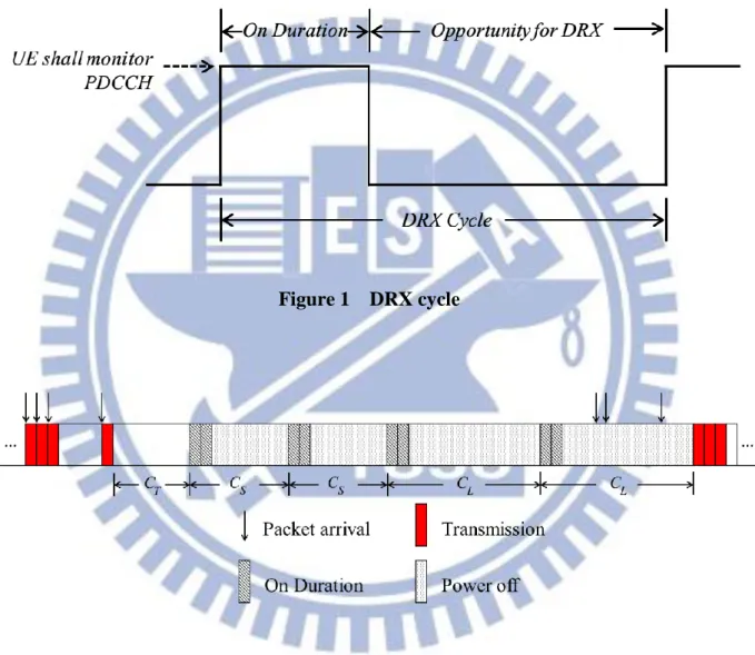
In LTE networks, different types of control and user data transmissions are served by a set of logic channels. Among the control channels, Physical Downlink Control Channel (PDCCH) is used for downlink data indication. The PDCCH carries downlink data allocation information and UE monitors and decodes PDDCH in each sub-frame (or millisecond) to check if there is any downlink data designated to it. According to LTE MAC protocol specification [2], an UE may be configured by RRC with DRX functionality to control the UE’s PDCCH monitoring activity. Once DRX is configured, UE is allowed to monitor the PDCCH discontinuously; otherwise, UE monitors the PDCCH continuously.

RRC controls DRX operation by configuring five major parameters, namely, On Duration Timer T , Inactivity Timer _on C , Long Cycle Length _T C , Short Cycle Length _L C and Short _S

Cycle TimerN_SC. If DRX is configured, the Inactivity Timer will be reset after each data transmission. When Inactivity Timer expires, that is UE has no data transmission for C _T

milliseconds, DRX operation enters sleeping state where discontinuous PDCCH monitoring takes place. During the sleeping state, DRX first adopts Short Cycle as DRX Cycle, and then migrate to Long Cycle after N_SC consecutive Short Cycles without receiving any downlink data indication. The Short Cycle is an optional functionality; in other words, it is allowed to set N_SC to zero. During On Duration of each cycle, UE has T milliseconds to monitor _on

(15)

monitoring, that is On Duration, in each cycle is determined by another parameter, DRX Start Offset. The Start Offset is designed for network to share the time among UEs with DRX, and for convenience, each Short or Long Cycle is assumed to start with an On Duration as shown in Figure 1. Moreover, an example of DRX mechanism with Short Cycle Timer N_SC 2 is illustrated in Figure 2.

Figure 1 DRX cycle

Figure 2 Example of DRX mechanism

1.3 Related Works

(16)

efforts have been made to analyze the performance of DRX mechanism. In [12], the authors proposed an analytical model assuming that packets arrive at the system according to a Poisson process and the transmission time of each packet is generally distributed. The model was extended in [13], [14], [15] for different goals and some analyses involved Z and

Laplace transforms. The derivations are quite complicated. A more general traffic model, the ETSI bursty data traffic model, which is widely used in various analytical and simulation studies of 3GPP networks, was adopted in [16]. Another recent research [17] derived the DRX performance metrics based on the concept of regenerative cycles. This approach is much easier than using Z and Laplace transforms. A drawback of the above previous studies

is that only the average packet delay was derived, which may not be applicable as a QoS requirement of real-time applications.

1.4 Structure of the Thesis

In this thesis, only downlink traffic is considered. Power saving performance and packet loss ratio of DRX mechanism with a real-time Poisson traffic are analyzed by combining Short and Long Cycles as a regenerative cycle. Instead of average packet delay, the packet loss ratio of DRX mechanism is derived, which is more realistic when verifying the quality of service under a system. Moreover, a procedure of DRX parameter setting is also proposed. Both numerical analysis and suggested configuration are verified, respectively, with computer simulation and optimum setting. The structure of thesis is organized as follows.

First in the beginning of Chapter 2, the analysis approach similar to [17] is described, followed by formulation of target metrics of packet loss ratio and power saving efficiency. The remaining part of the chapter includes derivations of variables required in the target metrics.

(17)

In Chapter 4, curves of analytical results and computer simulation with different values of DRX parameters are plotted for verification. The comparison between optimum DRX configuration and proposed approach is also presented in this chapter. Finally, the conclusion of this thesis is organized in Chapter 5.

(18)

Chapter 2 Analysis

2.1 Regenerative Cycle

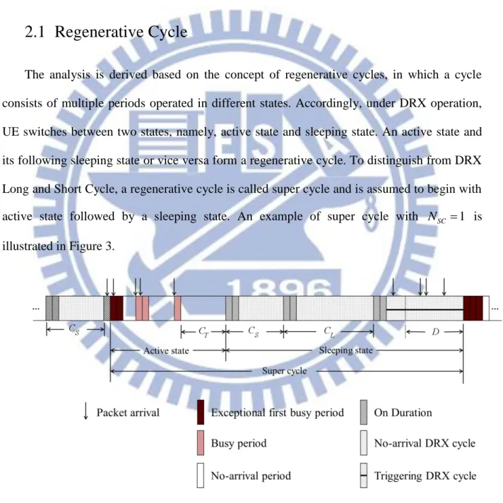
The analysis is derived based on the concept of regenerative cycles, in which a cycle consists of multiple periods operated in different states. Accordingly, under DRX operation, UE switches between two states, namely, active state and sleeping state. An active state and its following sleeping state or vice versa form a regenerative cycle. To distinguish from DRX Long and Short Cycle, a regenerative cycle is called super cycle and is assumed to begin with active state followed by a sleeping state. An example of super cycle with N_SC 1 is illustrated in Figure 3.

Figure 3 Example of super cycle

(19)

zero) busy periods, and ends with a period of length specified by Inactivity Timer. The exceptional first busy period is created by pending packets which arrived during sleeping state. Each busy period is created by a single packet arrival, and every busy period is preceded by a time period of length shorter than C without any packet arrival. Finally, the length of the _T

inactivity period is C and there is no packet arrival in this period. _T

During DRX Short and Long Cycles, UE periodically wakes up for T milliseconds and _on

listens to PDCCH for traffic indication. UE stays in sleeping state if the current DRX cycle is a no-arrival cycle; that is, there is no packet arrival in the current DRX cycle. Note that some packet arrivals may be dropped due to violation of delay bound constraint in a no-arrival cycle.

In contrast, UE enters active state from sleeping state if the current DRX cycle is a triggering cycle; in other words, at least one packet, which does not violate the QoS requirement, arrives in the current DRX cycle. To summarize, the sleeping state consists of some (could be zero) no-arrival DRX cycles and one triggering DRX cycle. In this study, packets could be discarded because of QoS violation. As a result, it is possible that all packets arrived at a DRX cycle are dropped. Under this circumstance, the DRX cycle is considered as a no-arrival cycle because UE does not know there are downlink packet arrivals.

2.2 Target Metrics

In this thesis, an UE is assumed that its packet arrival is a Poisson process with arrival rate  per millisecond. The arrival rate  is further assumed small that the possibility of having two or more packet arrivals within a sub-frame can be neglected. Also, the service time of each packet is deterministic and equals one millisecond, that is, each packet requires one millisecond to be served. The delay bound requirement of the traffic is denoted as D

(20)

milliseconds and there is a buffer which can store D packets is allocated in UE so that a

packet is dropped if and only if its arrival time preceding next active opportunity more than

D milliseconds.

To analyze the packet loss ratio of DRX mechanism, let M , ₁ M and ₂ M denote, ₃

respectively, the number of packet arrivals during the exceptional first busy period, the busy periods and the sleeping state. Also, let N represent the number of packets dropped in a

super cycle. Since a super cycle consists of one exceptional first busy period, some busy periods and a complete sleeping state, the total number of packet arrivals in a super cycle equals M₁M₂M₃. With the amount of packets dropped in a super cycle, the packet loss ratio of a super cycle p can be represented as

 





 

   

 

1 2 3 1 2 3

E N

p

E M

M

E N

E M









.

(1)

To deal with the power saving performance of DRX mechanism, one can analyze by the duration UE spends in active state and sleeping state. Let T and _A T be two random _S

variables that denote the lengths of active state and sleeping state in a super cycle, respectively. Moreover, let T_{S on}_{_} be the random variable representing the length of On Duration where UE should power on in the sleeping state. Therefore, the UE power saving efficiency e can be derived as ratio of the duration UE powered off to the length of a super cycle as shown in equation (2).

(21)





 

   

_ _ S S on S A S S on S A

E T

T

e

E T

T

E T



















 







(2)

In the following sections, the packet loss ratio shall be derived first, followed by the analysis of power saving efficiency.

2.3 Analysis of Packet Loss Ratio

One can note that the random variables in equation (1) are independent to each other. Therefore, the packet loss ratio can be derived by calculating E N ,

 

E M ,

 

1 E M

 

2 and

 

3

E M separately. In the scope of this thesis, the packet arrival rate  is small that the possibility of having more than one packet arrival in one millisecond can be ignored. For an UE with traffic following Poisson process, one can have that ee 1.

Note that if packet arrives in the th

i sub-frame of the On Duration where 1 i T_on1, the active state starts from the (i1)th sub-frame; otherwise, the active state begins right after the end of the current DRX cycle if the packet arrives at the (T_on)th sub-frame of the On Duration. Let G denote the probability of having one or more packet arrivals in the first

(T_on 1)sub-frames of On Duration and thus,

( 1)

1

Ton

G

 

e

 

.

(3)

To denote the time interval from the (T_on)th sub-frame to the end of current Short or Long DRX cycle, let

(22)

1

S S on

C

 

C



T



,

(4)

1

L L on

C

 

C



T



.

(5)

Further let s , _k l and _k d stand for , respectively, the probabilities of having _k k

packet arrivals in a time period of length C_S, C_L and D , for k0. One can infer that

(

)

!

S C k S k

C

e

s

k





 



,

(6)

(

)

!

L C k L k

C

e

l

k





 



,

(7)

(

)

!

k D k

D e

d

k







.

(8)

Since a packet shall be dropped if it is buffered for a time period longer than the delay bound requirement, the time interval C_S and C_L are divided into two segments, respectively, if C_S D and C_L D. For time interval C_S, the first segment is of length

S

C  D and the second one is of length D . In the same way, the time interval C_L is divided into two segments with the first one of length C_L D and the second one of length

D .

2.3.1 Derivation of

E M

 

₁

For convenience, one additional random variable K is introduced to represent the

number of buffered packets when UE enters active state from sleeping state, that is, the number of buffered packets right before the exceptional first busy period. Since one buffered

(23)

packet creates one busy period, K buffered packets will create K busy periods. With the

fact that the average number of packets served in a busy period is

1 / (1





)

[10], the average number of packet arrival during exceptional first busy period is

 

1

1 E K

E M

E K











.

(9)

To compute E K , three cases are considered separately below.

 

Case 1. C_SC_LD

For C_SC_LD, no packet arrival will be dropped in a DRX cycle. In other words, the first DRX cycle with packet arrival(s) is the triggering cycle. E K can be derived by

 

calculating the cases of having first arrival in different DRX cycles, such as the first N_SC

Short Cycles and the following Long Cycles. Therefore,

1 1 1 2 1 1 1 1

[ ] [

(1

)

]

[

(1

)

]

(

) [

(1

)

]

(

)

[

(1

)

]

(

)

[

(1

)

] (

)

[

(1

)

]

(

)

(

)

S S S S S S S SC L L S SC S SC L S SC L C C C k k k k C C C C N k k k k C C C N C N C k k k k C N C

E K

G

s

k

e

G

s

k

e

G

s

k

e

G

s

k

e

G

l

k

e

G

l

k

e

                            



 

 

 





 

 



 





 

 

 







2 1

[

(1

)

]

L C k k

G

l

k

 

 



 

. (10)

(24)

1 1 0 1 0

[ ] [

(1

)

]

(

)

(

)

[

(1

)

]

(

)

1

1 [

(1

)

]

(

)

[

(1

)

]

1

1 (1

)

(1

)

(1

)

1

S SC L S S SC L S SC S SC S L S SC S SC S C N C C i C N C i k k k i k i C N C N S C L C C N S C N L C

E K

G

s

k

e

G

l

k

e

G

C

e

G

C

e

G

C

G

C

e

         



 _  _              



 





 









 



 





 

 







L C

e





(11)

Case 2. C_S D C_L

For C_S D C_L, during DRX Long Cycles, packets which arrive in the first segment of C_L shall be discarded. Therefore,

 

1 1 0 1 0 1 2 0 1

[

(1

)

]

(

)

(

)

[

(1

)

]

(

)

[(1

)

][

(1

)

]

(

)

[(1

)

] [

(1

)

]

S SC S S SC S SC S SC C N C i k k i D C N k k D C N k k D C N k k

E K

G

s

k

e

G

d

k

e

G d

G

d

k

e

G d

G

d

k

              



 





 







 







 

 



.

(12)

(25)

 

1 0 1 0 1 0 0

[

(1

)

]

(

)

(

)

[

(1

)

]

[(1

)

]

1

1 [

(1

)

]

(

)

[

(1

)

]

1 1 (1

)

(1

)

(1

)

(1

)

1 1 (1

S SC S S SC S SC S SC S S SC S SC S C N D C i C N i k k k i k i C N C N S C C N S C N C

E K

G

s

k

e

G

d

k

G d

e

G

C

e

G

D

e

G d

G

C

G

D

e

       



 _ _            



 





 









 



 



 



 

 







0

)

G d



.

(13)

Case 3. DC_SC_L

For DC_SC_L, packets arriving in the first segments of C_S and C_L are dropped. With the same idea above, one can derive

 













1 0 1 0 0 0 1 0 0 0 0 0 0 0 0

[

(1

)

]

[(1

)

]

[(1

)

]

[

(1

)

]

[(1

)

]

1 (1

)

1 [

(1

)

]

[(1

)

]

[

(1

)

]

1 (1

)

1 (1

)

(1

)

(1

1 (1

)

(1

)

1 (1

)

SC SC SC SC SC SC N D i k k i D N i k k i N N N N

E K

G

d

k

G d

G

d

k

G d

G

D

G d

G

D

G d

G

D

G

G d



     



 





 





 



 





 

 

 

 







 



0

)

1 (1

)

G

D

G d



 

.

(14)

By substituting E K into equation (10), the results of

 

E M under different cases

 

1

shall be acquired.

2.3.2 Derivation of

E M

 

₂

(26)

deterministic packet service time, no packet will be dropped during the active state. If there is no packet arrival in time interval of length

C

_T, an UE terminates the active state; otherwise, a packet arrival creates a busy period and resets the Inactivity Timer. Since the average number of packets served in a busy period equals to

1 / (1





)

, one can derive the average number of packet arrivals before expiration of Inactivity Timer as follows.

 

2

 

2

1

0 (1

)(

)

1

1 (1

)

T T T T C C C C

E M

e

E M

e

   



   



  









(15)

2.3.3 Derivation of

E M

 

₃

Derivation of E M

 

3 is similar to that of E K . In the same way, three cases are

 

considered respectively.

Case 1. C_SC_LD

Under the assumption that the chance of having two or more packet arrivals in a sub-frame can be neglected, one can infer that no packet will be dropped in the sleeping state if C_SC_LD. Therefore, E M

 

₃ equals to E K for case 1.

 

3

(1

)

(1

)

(1

)

1

S SC S SC S L C N S C N L C C

G

C

G

C

E M

e

   



   



 

 





(16)

Case 2. C_S D C_L

The equation for E M

 

3 in case 2 is the same as that for E K , except the term

 

(27)

considering the packet arrivals in the second segment of C_L for E K , the arrivals in both

 

first and second segments should be taken into account when calculating E M

 

₃ .

 

3 0

(1

)

(1

)

(1

)

1 1 (1

)

S SC S SC S C N S C N L C

G

C

G

C

E M

e

G d

  



  



 

 





 

(17)

Case 3. DC_SC_L

Similar to case 2, for DC_SC_L, the equation for E M

 

3 is the same as that for

 

E K , except the terms [G (1 G)D] in (14) are replaced with [G (1 G)C_S] for the first one and [G (1 G)CL] for the second one.

 

3



0





0



0 0

(1

)

(1

)

1 (1

)

(1

)

1 (1

)

1 (1

)

SC SC N

G

C

_S N

G

C

_L

E M

G d









 

 







 

(18)

2.3.4 Derivation of

E N

 

Recall that M₃ and K represent the number of buffered packets, respectively, in the

whole sleeping state and right before the beginning of active state. Since packets can only be discarded in sleeping state, the number of dropped packets in a super cycle shall be the difference of M₃ and K . Thus, one can get NM₃K, which implies

 

   

3

E N



E M



E K

.

(19)

With the equations for E M ,

 

₁ E M

 

2 , E M

 

3 as well as E N , the packet loss

 

(28)

2.4 Analysis of Power Saving Efficiency

To obtain the power saving efficiency, three equations for E T

 

A , E T

 

S and

_

S on

E T_ _ are required in (2). The equations are derived below separately.

2.4.1 Derivation of

E T

 

_A

The length of the active state in a super cycle consists of three parts, namely, the length of exceptional first busy period, busy periods and an Inactivity Timer. The expected length of exceptional first busy period equals to E K

 

/ (1) because, on the average, it is created with E K packets. Similarly, the expected length of a busy period equals

 

1/ (1) and each busy period is preceded by a no-arrival period shorter than the Inactivity Timer. The average length of the no-arrival period can be derived as follows.

0 0 2 0 0

1

1 (

1)

1

1 (

1)

1

1 [

(

1)

]

1

1 [ (1

)

]

1

T T T T T T T T T T T T T T t C C _t C C C t C t C t C t C T C C C T C T C

te

dt

te

dt

e

t

e

t

e

C

e

C

e

C

e

             



_



              









 







 









 









 





(20)

One can infer from (15) that the average number of busy periods in an active state is

(1



_e

CT

) /

_e

CT_{. Combining the lengths of the first exceptional first busy period, the busy}

(29)

periods and the last Inactivity Timer, E T

 

_A can be derived as

 

1

1 [

]

1

1 (

1)

(1

)(

1)

(1

)

[

]

1 (1

)(

1)

1

1 (1

)

[

]

1 (

1)

(1

)

1 (1

)

(1

)

[

1 (

T T T T T T T T T T T T T C T A C C T C C C T T C C C C T T C C C T T

E K

e

C

E T

C

e

E K

e

C

e

E K

e

C

e

E K

e

C

            



 



     







 





  

 









 









 













 

2

]

1 )

1

T C

E K

e



 









. (21)

2.4.2 Derivation of

E T

 

_S

Let g represent the probability of having one packet arrival in one millisecond and H

denote the expected duration before entering active state during the first (T_on 1) On Duration sub-frames.

g





e



(22)

1 1 1

(1

)

on T k k

H

g

g k

  









(23)

As the calculation of E M

 

2 , three different cases are considered separately.

Case 1. C_SC_LD

(30)

 

1 0 0

[

(1

)

]

(

)

(

)

[

(1

)

]

(

)

1

1 [

(1

)

]

[

(1

)

]

1

1 (1

)

(1

)

(1

)

1

SC S S SC L S SC S SC S L S SC S SC S L N C k S S k C N C k L k C N C N S C L C C N S C N L C C

E T

H

G C

e

H

G C

e

H

G C

e

H

G C

e

H

G C

H

G C

e

                         



 



 





 



 



 

 







. (24)

Case 2. C_S D C_L

For C_S D C_L, one can have

 

1 0 0 0 0

[

(1

)

]

(

)

(

)

[

(1

)

]

[(1

)

]

1

1 [

(1

)

]

[

(1

)

]

1 1 (1

)

(1

)

(1

)

(1

)

1 1 (1

)

SC S S SC S SC S SC S S SC S SC S N C k S S k C N k L k C N C N S C L C N S C N L C

E T

H

G C

e

H

G C

G d

e

H

G C

e

H

G C

e

G d

H

G C

H

G C

e

G d

                   



 



 





 



 



 

 

 





 



. (25)

Case 3. DC_SC_L

(31)

 

1 0 0 0 0 0 0 0 0 0 0 0 0

[

(1

)

]

[(1

)

]

[(1

)

]

[

(1

)

]

[(1

)

]

1 ((1

)

1 [

(1

)

]

[(1

)

]

[

(1

)

]

1 (1

)

1 (1

)

(1

)

(1

)

[1 ((1

)

]

((1

)

1 (1

)

1

SC SC SC SC SC SC N k S S k N k L k N N S L N S N L

E T

H

G C

G d

H

G C

G d

H

G C

G d

H

G C

G d

H

G C

H

G C

G d

   



 



 





 





 

 

 

 







 



0

(1

G d

)

 

.

(26)

2.4.3 Derivation of

E T



_

_S_{_}_on



_

The equation for E T_ _{S on}_{_} _ is similar to that for E T . Since only the length of On

 

_S

Durations contribute to E T_ _{S on}_{_} _, the two terms [H (1 G C) _S] and [H (1 G C) _L] in (24), (25) and (26) are both replaced with [H (1 G T) _on].

Case 1. C_SC_LD _

(1

)

(1

)

(1

)

1

S SC S SC S L C N on C N on S on C C

H

G T

H

G T

E T

e

       

 



  







_

(27)

Case 2. C_S D C_L _ 0

(1

)

(1

)

(1

)

1 1 (1

)

S SC S SC S C N on C N on S on C

H

G T

H

G T

E T

e

G d

     

 



  







_

_{ }

(28)

Case 3. DC_SC_L _ 0 0 0 0

(1

)

(1

)

[1 ((1

)

]

((1

)

1 (1

)

1 (1

)

SC SC N on N on S on

H

G T

H

G T

E T

G d

 



  











_{ }

(29)

(32)

As the equations for E T

 

_A , E T and

 

_S E T_ _{S on}_{_} _ are derived, the power saving efficiency e can be calculated by substituting the expected values in (2).

A DRX performance simulator is also created in this work. Before verifying the accuracy of equations derived above, a configuring procedure for DRX parameters based on observations from DRX simulator is proposed in next chapter.

(33)

Chapter 3 QoS Support

3.1 Proposed DRX Parameters Configuration

Table 1 lists the available values of DRX parameters which are specified in the LTE-Advanced standard document [3].

Table 1 Available Values of DRX Parameters

Parameter Values

On Duration (T ) on 1, 2, 3, 4, 5, 6, 8, 10, 20, 30, 40, 50, 60, 80, 100, 200 (ms)

Inactivity Timer (C ) _T 0, 1, 2, 3, 4, 5, 6, 8, 10, 20, 30, 40, 50, 60, 80, 100, 200, 300,

500, 750, 1280, 1920, 2560 (ms)

Long Cycle Length (C ) L

10, 20, 32, 40, 64, 80, 128, 160, 256, 320, 512, 640, 1024, 1280, 2048, 2560 (ms)

Short Cycle Length (C ) _S 2, 5, 8, 10, 16, 20, 32, 40, 64, 80, 128, 160, 256, 320, 512,

640 (ms) Short Cycle Timer (N_SC) Integer{1, …, 16}

With all the possible values, there are hundreds of thousands of combinations can be achieved. Based on the analysis in previous chapter, an approach to configuring the DRX mechanism with Poisson arrival traffic is proposed. The initial design intension of introducing these five parameters is not mentioned in the specification document. Thus, the purposes of

(34)

each parameter are designed based on the proposed approach.

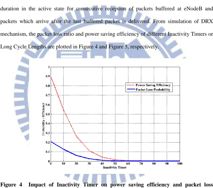
First, On Duration is mainly for indication of downlink traffic and can be set with a small value by assuming that the scheduler of eNobeB is well designed to allocate resource precisely within the On Duration. The small value can be 2 or 3 milliseconds and is set to 2 ms in the following verification. The goal of Inactivity Timer is assigned to extend the duration in the active state for consecutive reception of packets buffered at eNodeB and packets which arrive after the last buffered packet is delivered. From simulation of DRX mechanism, the packet loss ratio and power saving efficiency of different Inactivity Timers or Long Cycle Lengths are plotted in Figure 4 and Figure 5, respectively.

Figure 4 Impact of Inactivity Timer on power saving efficiency and packet loss probabilty for = 0.1 , T_on = 2 ms , C_L= 256 ms , C_S = 16 ms , N_SC = 2 with

= 100 ms

(35)

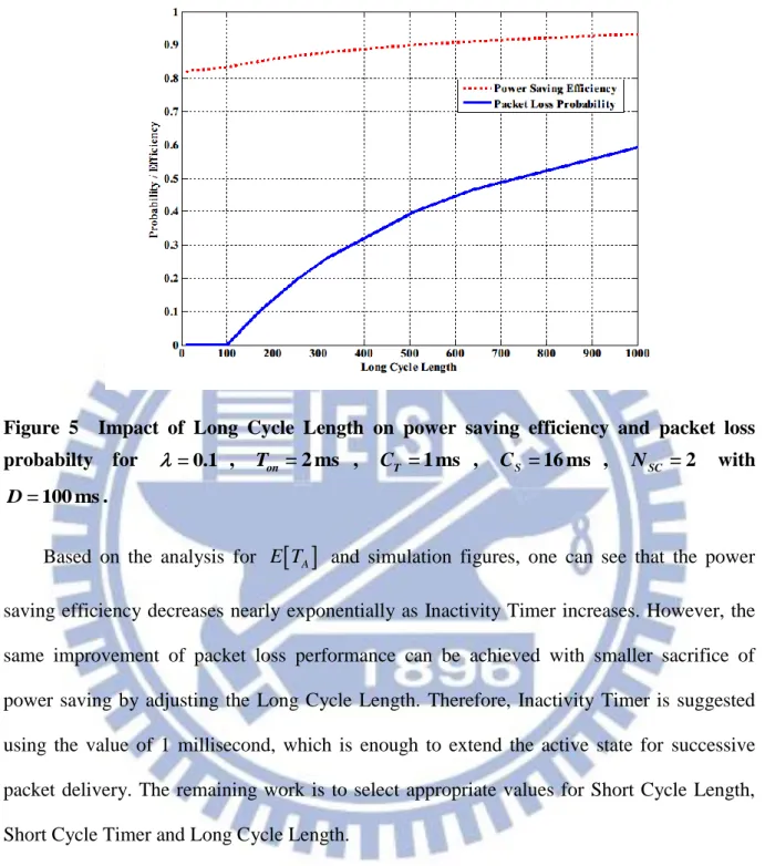
Figure 5 Impact of Long Cycle Length on power saving efficiency and packet loss probabilty for  = 0.1 , T_on = 2 ms , C_T = 1 ms , C_S = 16 ms , N_SC = 2 with

= 100 ms

D .

Based on the analysis for E T

 

A and simulation figures, one can see that the power

saving efficiency decreases nearly exponentially as Inactivity Timer increases. However, the same improvement of packet loss performance can be achieved with smaller sacrifice of power saving by adjusting the Long Cycle Length. Therefore, Inactivity Timer is suggested using the value of 1 millisecond, which is enough to extend the active state for successive packet delivery. The remaining work is to select appropriate values for Short Cycle Length, Short Cycle Timer and Long Cycle Length.

It is obvious that to achieve maximum power saving performance, one should choose parameter values so that the packet loss probability is as close as possible to but no greater than the QoS requirement. Moreover, given the desired packet loss probability, the proportion of time UE has to be powered on to receive packets is a constant. Therefore, to achieve higher energy saving performance, the chances of having idle On Durations should be reduced. Since

(36)

Short Cycles have higher possibility to generate idle On Durations, the suggestion is to set DRX mechanism without any Short Cycles, leaving only Long Cycle Length to be configured.

Finally, the Long Cycle Length is selected to be the one that maximizes the power saving efficiency subject to the constraint of QoS requirement. Because there are only 16 possible values for Long Cycle Length, one can choose the optimum values using exhaustive search by substituting each value options into the equation of packet loss ratio.

(37)

Chapter 4 Verification

In this chapter, the analyses are verified with computer simulation and the suggested DRX selection is also compared with the optimum configuration.

4.1 Verification of Numerical Analysis

The numerical results of packet loss probability and power saving efficiency are verified with the simulation. In the following comparisons, four DRX parameters, that is, Long Cycle Length, Short Cycle Length, Short Cycle Timer and Inactivity Timer are adjusted respectively, leaving three other parameters fixed in each comparison. Cases of 0.01 and  0.1 are both considered. In general, compared to the case of  0.1, the case of 0.01results higher packet loss probability and power saving efficiency with the same configuration.

(38)

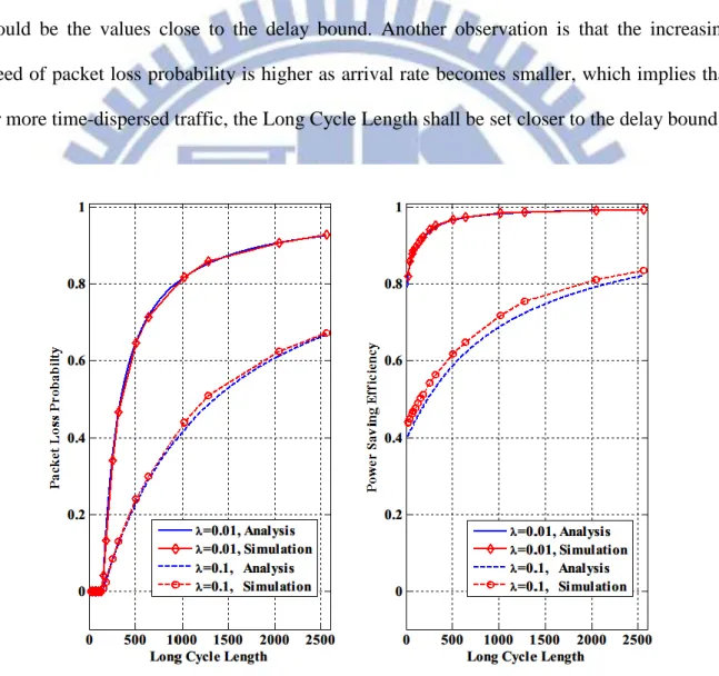
First in Figure 6, the value of Long Cycle Length is a variable. As one can see, the analytical results match well with simulation results. There is no packet dropped before the value of Long Cycle Length exceeds the delay bound requirement, that is, 150 milliseconds. As Long Cycle Length increases, both packet loss probability and power saving efficiency increase. The packet loss probability increases rapidly once the Long Cycle Length exceeds the delay requirement. Therefore, it can be inferred that the appropriate Long Cycle Length should be the values close to the delay bound. Another observation is that the increasing speed of packet loss probability is higher as arrival rate becomes smaller, which implies that for more time-dispersed traffic, the Long Cycle Length shall be set closer to the delay bound.

Figure 6 Packet loss probabilty and power saving efficiency with different Long Cycle Lengths for  = 0.01 , 0.1, T_on = 2 ms, C_T = 10 ms, C_S = 16 ms, N_SC = 2, D= 150 ms.

(39)

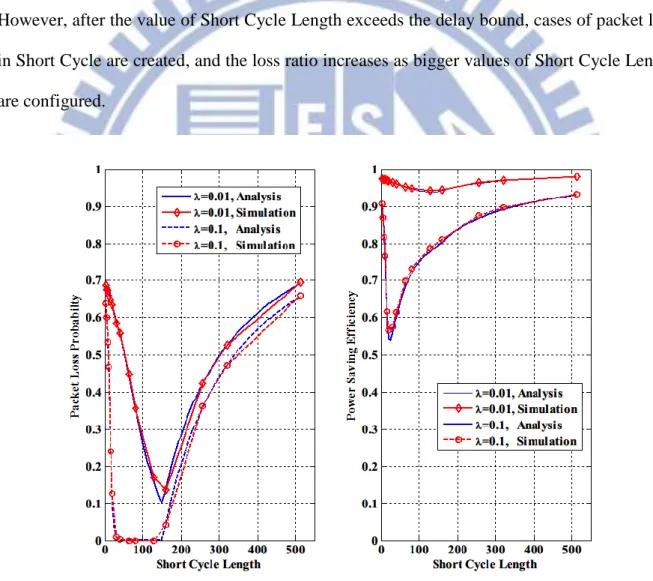
In Figure 7, comparisons with different Short Cycle Lengths are conducted. The analytical and simulation results are still matched. One can discover that the DRX performance varies dramatically as Short Cycle Length differs. In case of 0.1, if a small value of Short Cycle Length is adopted, the DRX tends to enter Long Cycle more easily because there is good possibility of having no-arrival Short Cycles. As Short Cycle Length rises, there is a zone with much lower packet loss probability where Short Cycle Length is long enough to capture most packet arrivals, mitigating the packet loss in Long Cycle. However, after the value of Short Cycle Length exceeds the delay bound, cases of packet loss in Short Cycle are created, and the loss ratio increases as bigger values of Short Cycle Length are configured.

Figure 7 Packet loss probabilty and power saving efficiency with different Short Cycle Lengths for  = 0.01 , 0.1, T_on = 2 ms , C_L= 512 ms , C_T = 10 ms , N_SC = 2,

= 150 ms

(40)

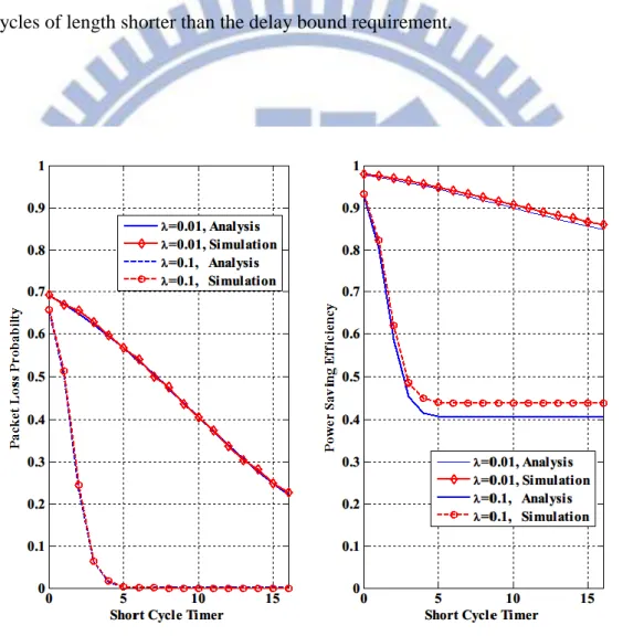
In Figure 8, the Short Cycle Timer is a variable. In case of 0.1, there is a lower bound both in packet loss probability and power saving efficiency with Short Cycle Timer of values bigger than five. The reason is that with the parameter configuration described in Figure 8, the chance of having packet arrivals, whose inter-arrival times are greater than the length of five or more consecutive Short Cycles, can be neglected; in other words, only Short Cycles are executed in this case. Therefore, no packet will be dropped if all packets arrive in Short Cycles of length shorter than the delay bound requirement.

Figure 8 Packet loss probabilty and power saving efficiency with different Short Cycle Timers for  = 0.01 , 0.1, T_on = 2 ms , C_L= 512 ms, C_S = 16 ms, C_T = 10 ms,

= 150 ms

(41)

Comparisons with Inactivity Timer being adjustable parameter are shown in Figure 9 and the analytical analysis matches the simulation result. As discussed in previous chapter, the power saving efficiency decreases severely as Inactivity Timer increases for the case of

0.1

  . To lower packet loss probability, one can adjust DRX by decreasing Long Cycle Length or Short Cycle Length. Increasing Short Cycle Timer or Inactivity Timer are also other alternatives. However, with the same improvement of packet loss probability, one can see that the adjustment by increasing Inactivity Timer will cause severe degradation on power saving efficiency. Therefore, it is suggested to set Inactivity Timer to some small values for Poisson arrival process.

Figure 9 Packet loss probabilty and power saving efficiency with different Inactivity Timers for  = 0.01 , 0.1 , T_on = 2 ms , C_L= 512 ms , C_S = 16 ms , N_SC = 2 ,

= 150 ms

(42)

4.2 Verification of Proposed Configuration

One can infer that the trade-off between packet loss probability and power saving efficiency can be achieved by adjusting any DRX parameter. However, the simplicity of parameter configuring approach should also be considered. The approach proposed in previous chapter manages to raise the power saving efficiency as high as possible by only adjusting DRX Long Cycle under the constraint of QoS requirement, and is expected to be an eligible method for Poisson arrival process. For verification of proposed approach, optimum configuration is obtained by brute force search, and the performance of proposed approach is shown in Figure 10.

Figure 10 Performance comparison between proposed DRX configuration and optimum DRX configuration for D= 100, 150 ms and  = 10%.

長期演進技術中非連續接收機制之服務品質與省電效能分析

國 立 交 通 大 學

電信工程研究所

碩 士 論 文