智慧行動裝置上之擴增實境定位技術

國

立

交

通

大

學

資訊科學與工程研究所

碩

士

論

文

智 慧 行 動 裝 置 上 之 擴 增 實 境 定 位 技 術

AR-based Positioning on Mobile Devices

研 究 生：鄭淵舟

指導教授：易志偉 教授

智慧行動裝置上之擴增實境定位技術

AR-based Positioning on Mobile Devices

研 究 生：鄭淵舟 Student：Yuan-Chou Cheng

指導教授：易志偉 Advisor：Chih-Wei Yi

國 立 交 通 大 學

資 訊 科 學 與 工 程 研 究 所

碩 士 論 文

Submitted to Institute of Computer Science and Engineering College of Computer Science

National Chiao Tung University in partial Fulfillment of the Requirements

for the Degree of Master

in

Computer Science

July 2012

Hsinchu, Taiwan, Republic of China

智慧行動裝置上之擴增實境定位技術

學生：鄭淵舟

指導教授：易志偉 教授

國立交通大學

資訊科學與工程研究所

摘要

AR-based Positioning for Mobile Devices

Student：Yuan-Chou Cheng

Advisors：Prof. Chih-Wei Yi

Institute of Computer Science and Engineering

National Chiao Tung University

Abstract

Augmented Reality (AR) can be used to enrich LBS application by utilizing

position and orientation information from a location database of POIs. The AR

technique is suitable to develop intuitional Pedestrian Navigation Systems (PNSs).

Higher positioning accuracy is needed for displaying AR objects at proper places.

However, current commercial positioning solutions, such like outdoor GPS and

indoor RF systems, cannot provide required positioning accuracy. In this paper, we

propose an AR-based positioning technique for AR users to locate their current

locations. First, by utilizing a coarse positioning system, AR objects can be roughly

displayed on the touch screen of an AR device. Then, AR objects can be matched with

coordinates of the AR objects in the image and in the real world can be known. Based

on the coordinates and the known camera focal length, the location at which the

photograph was taken can be obtained. The location of the camera can be treated as

the location of the user. The proposed positioning technique is very helpful in

誌 謝 我要感謝我的指導教授，易志偉教授，在我碩士生涯這兩年給我很多的指導 跟鼓勵，並且提供了我良好的實驗室環境，讓我得以順利完成此篇論文。 再來，我由衷的感謝我的指導學長林巨益，在研究上提供很多建議與指導。 另外，也感謝NOL的全體同學，在這兩年來給我的鼓勵與幫助。 最後，我要感謝我的父母以及所有關心我的人對我付出的關懷與期許，使我 在挫折的時候可以再度站起來，度過最困難的時光。真的謝謝大家，因為有你們 的幫忙跟鼓勵，讓我可以在碩士兩年的生涯學到很多也經歷很多，留下許多美好 的回憶。謝謝! 鄭淵舟 於 國立交通大學資訊科學與工程研究所碩士班 中華民國101年7月

Contents

1 Introduction 1

2 Related Work 4

3 The View Angle and Geometry between Camera and Objects 8

3.1 The Principle of Photo-Imaging . . . 9

3.2 View Angles between Objects . . . 11

3.3 Geometry between Camera and Objects . . . 13

4 AR-based Positioning 15 4.1 View Angle Algorithm . . . 16

4.1.1 The Proposed Gradient Algorithm . . . 17

4.2 Similar Triangle Algorithm . . . 18

4.3 Implementation Issues . . . 20

5 Experiment 22 5.1 Effective Focal Length (EFL) Experiment . . . 22

5.1.1 EFL Experiment of View Angle Algorithm . . . 23

5.1.2 EFL Experiment of Similar Triangle Algorithm . . . 24

5.2 AR-P Experimental Results . . . 30

List of Figures

3.1 The relation of object distance, image distance and focal length. . . 9

3.2 The coordinate layout of an image. . . 11

3.3 The view angle between P1 and P2. . . 12

3.4 Geometry between user and objects . . . 13

4.1 User Interface of AR-Positioning . . . 15

5.1 The coordinates and arrangement of A, B, C, D and E. . . . 23

5.2 Test lines of experiment . . . 26

5.3 Similar triangles relation among camera and POIs . . . 27

5.4 The effective focal length with different camera distance Dc . . . 28

5.5 Long line and short Line . . . 28

5.6 Average testing focal length and trend line and trend line . . . 29

5.7 Experiment locations in map . . . 31

5.8 AR-P experiment environment . . . 31

5.10 Similar Triangle algorithm result: positioning error affected by focal length . 33

5.11 Average positioning results with different test locations . . . 34

5.12 Positioning result affected by combinations number . . . 34

5.13 Local minima with 3 points . . . 35

5.14 Local minima with 7 points . . . 35

5.15 View Angle algorithm: Positioning error affected by combination numbers . 36 5.16 Positioning error affected by POI combinations of same plane . . . 37

5.17 Positioning error affected by combinations of distant POI . . . 38

5.18 Positioning result affected by POI combinations . . . 38

5.19 Positioning error affected by combinations of distant POI . . . 39

5.20 Poor positioning results due to closed combinations . . . 39

5.21 Position function with 2 points, A and B. . . 40

5.22 Solutions of equations. . . 42

5.23 The x, y, z result of test Location 1 in AR frame . . . 43

List of Tables

5.1 The view angles between objects (in degrees). . . 24

5.2 The coordinates (in cm) of A, B, C, D and E in the images. . . . 25

Chapter 1

Introduction

Augmented Reality (AR) adds on graphics, text objects or sound called AR objects, to enrich digital images and provide interactivity among users. We propose two AR-based positioning algorithms, View Angles algorithm and Similar Triangles algorithm, to locate current position of users. However, it will need the rough location and heading information of user to render AR objects properly on mobile devices.

Nowadays, most smartphones and tablet devices are equipped with a digital camera to take photographs, a GPS receiver for positioning, a m-sensor to detect orientation, a LCD touch screen to interact with users, and a WiFi/3G/4G interface to access Internet. All the mentioned built-in devices of mobile device meet the requirements of being an AR platform for AR applications. Due to the explosive growth of smartphones and tablet devices, AR will become an important Human Computer Interface (HCI). For rendering AR objects at right places, we need a positioning system to provide location information. The most

popu-lar positioning technologies for smartphones include GPS/GNSS, Cell Tower Triangulation, WiFi-RSS-based positioning, etc. However, the positioning accuracy of those technologies are not precise enough for some AR applications. This problem becomes worse if point-of-interest (POI) are close to the users. The inaccuracy of positioning systems is a major barrier for AR applications. In this work, we propose an AR-based positioning technique that utilize a coarse positioning system and a location database of POIs to estimate the precise location of users. By the means, the rough location and orientation of the user who possesses the AR device is known.

The proposed idea is described as follows. First, by utilizing a coarse positioning system, AR objects of POIs are displayed close to the images of the POIs on the touch screen. By dragging the AR objects and dropping them at the corresponding images on the touch screen, the AR objects are matched to the image of the POIs. The coordinates of the POIs in the real world can be known by querying the location database of POIs. In addition, the places where the AR objects are dropped give us the coordinates of the POIs in the image. From the coordinates of POIs and focal length of the camera lens, the position of user can be calculated by our proposed algorithm. Average positioning error of View Angle algorithm is from 88.9cm to 245.9cm. It is caused by the local minima issue of initial guess. Experiments show the Similar Triangle algorithm have average positioning error of 74.34cm. Similar Triangle algorithm do not have the problems of local minima and have a better positioning result compared with View Angle algorithm. The accuracy of our proposed algorithms are better than the accuracy of most positioning technologies on mobile devices [1][2].

In Chapter 3, we first introduce some preliminary background knowledge on photo-imaging including the principle of photo-photo-imaging, the concept of effective focal length, the calculation of view angles and geometry between user and objects. In Chapter 4, two AR-based Positioning (AR-P) problems are defined, and View Angle algorithm and Similar Tri-angle algorithm are proposed to solve the AR-P problems. In Chapter 5, experiment results are given to verify the proposed positioning algorithm. Conclusions are given in Chapter 6.

Chapter 2

Related Work

GPS [3] is the most popular outdoor positioning system. A GPS receiver determines its position by computing relative pseudoranges from multiple GPS satellites. The pseudoranges are calculated with multiplying the speed of light by the GPS signal transmission delay time measured between the GPS receiver and each satellites. By using satellites ephemeris data and at least four pseudoranges, it can triangulate current position of a GPS receiver. GPS provide Satellite clock, Ephemeris and Almanac to GPS receiver. GPS receivers use these information to synchronize time and calculate its moving speed, altitude, latitude and longitude. The advantages of GPS are wide coverage and popular End User navigation devices. However, the Ionospheric effects, Ephemeris errors, Satellite clock errors, Multipath distortion, Tropospheric effects and receiver error will effect the position accuracy of GPS. GPS also have application limitation in indoor environment or under bad weather. Some augmentation systems assist to improve accuracy of GPS, such like Assisted GPS (A-GPS)

[4], Differential GPS (DGPS) [5] and Wide Area Augmentation System (WAAS)[6].

There are several indoor positioning methods to locate the position of users, such like RF-based, ultrasound, infrared and RFID. The most popular one is RF-based due to the wide coverage of WLAN infrastructure. In RF-based indoor positioning, the RSS of time-of-arrival (TOA), angle-time-of-arrival (AOA) and radio propagation model are used to estimate the current location of users. RADAR is proposed in [7]. It is a radio-frequency RF-based

system for locating and tracking users inside buildings. RADAR operates by recording

and processing signal strength information at multiple base stations positioned to provide overlapping coverage in the area of interest. The RADAR method is used in RF-based positioning. The paper [8] proposes an approach using existing beacons to measure the RSSI from other beacons as a reference, which is called inter-beacon measurement, for the calibration of radio maps on the fly. The the statistical distribution of indoor RSS is not easy to characterize. In [9], it proposed the use of nonparametric statistical procedures for diagnosis of the fingerprinting model, which take into account the complex nature of the fingerprinting output. The framework of [10] can provide a valuable solution for pattern-matching localization which shows how to effectively build a radio map and quickly estimate the user’s location with acceptable distance errors. However, RF-based positioning has signal drift issue, its accuracy is not enough to display indoor AR objects at proper location.

Augmented reality [11] is proposed in 1992. The authors describe the design and proto-typing steps they have taken toward the implementation of a heads-up, see-through, head-mounted display (HUDset). Combined with head position sensing and a real world

registra-tion system, this technology allows a computer-produced diagram to be superimposed and stabilized on a specific position on a real-world object. In [12, 13, 14], by the help of laser pointers, image-based distance measurement techniques were proposed. Two laser pointers attached to a camera are used to emit laser beams that are parallel to the optical axis of the camera. By measuring the distance between the spots in the image of the two laser beams, the distance from the camera to the target object can be calculated if the distance between the two laser pointers and the focal lens of the camera are known. In [15], a nighttime vehicle distance measuring method based on a CCD image was proposed. By detecting the taillights of a target vehicle in the front based on image analysis, the distance to the front vehicle can be estimated from the distance between the taillights in the image. The proposed method works only during nighttime and more efforts are needed to distinguish the brands and types of target vehicles. In [16], a camera mounted on a moving platform whose motion and rotation velocities are available is used to estimate the distance. In [17], the distance be-tween an object and the camera lens is estimated by a parallax getting from multi-cameras. Additional cameras are needed to obtain the parallax. In [18], the photogrammetric six degrees of freedom (6DOF) pose estimation method was adopted to improve the positioning accuracy. In [19], the positioning procedure was performed in two phases: image-processing and pose estimation. In the image-processing phase, images taken in real time were matched with a 3D map to get the coordinates of objects. In pose estimation, camera position and orientation were determined by giving a set of correspondences between known 3D reference points and their 2D positions in images. Marker tracking is a general vision-based method

considering positioning issues in AR technology [20] [21]. They use each AR tag’s location as roughly user current location to recalculate the route. Visual markers usually impair the scenery and then some research focuses on tracking with invisible visual markers [22]. These systems provide some predefined visual or audio interactive action of each AR tags. It is a nice way to present dynamic route plan. However, it can not provide the high-precision location of user and correct route if user do not follow the predefined moving trajectory and marker pre-installment is also an overhead in such systems. Natural feature tracking is also a generally method in AR positioning [23] [24]. Navigation systems are developed by comparing the scene captured by a camera with predefined databases. However, in such systems, heavy computing loads of analyzing camera view is a major drawback. In our systems, these problems mentioned in marker based and vision-analyzed based method do not exist. We need not pre-install markers before and instead of the heavy computing load caused by comparing camera scene with database, interactivity by dragging-and-dropping POIs by user can solve these problems.

In the future work, we want to extend our system combined with feedback information routing (FIR) in [25] and other positioning technique such as GPS or WiFi positioning to implement an real-time and high accuracy indoor evacuation system in [26].

Chapter 3

The View Angle and Geometry

between Camera and Objects

The view angle and geometry between camera and objects are the key information in the proposal algorithm. In this chapter, we are going to introduce how to calculate the view angle and the geometry between camera and objects in an image. In Section 3.1, we introduce the basic principles of photo-imaging, including the thin lens equation and the concept of Effective Focal Length (EFL). In Section 3.2, we give the formula to calculate the view angle between objects in an image. The geometry between user and objects is illustrated in Section 3.3.

3.1

The Principle of Photo-Imaging

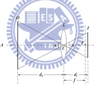
Figure 3.1 illustrates an example of photo-imaging. L is a positive lens whose focal length is f . C locating at the center of the lens L is the optical center of L. F is a focus of L. The distance between C and F , denoted as f , is the focal length of L. The line perpendicular to the lens and passing C and F , denoted as A, is the optical axis of L. O to the left of L is an object, and I to the right of L is the image of O with lens L. The distance between O

and L is called the object distance and denoted as do; and the distance between C and I is

called the image distance and denoted as di. The angle α is called the view angle of object

O. A L C O α α I F do di f

Figure 3.1: The relation of object distance, image distance and focal length.

The thin lens equation, Eq. (3.1), 1 do + 1 di = 1 f. (3.1)

we have di = 1 1−_df o f ≈ f. (3.2)

Especially, if do ≫ f, di can be approximated by f . Actually, this is the most case in

photographing, and we use f = di implicitly in the following discussion.

Taking a photograph, the image is recorded on a film gauge or converted by a CCD or CMOS device into electronic signal and saved as a file. Traditionally, the most popular film gauges are the 35mm still photography films that also known as 135 films. The size of 135

films is 35mm × 24mm. The ”angle of view” or ”field of view” of a photograph are the

diagonal angular extent of the scenes. To prevent possible ambiguity, we prefer the term field of view in what follows. If D is the diagonal of the film, the field of view can be obtained by

2 arctan D

2di

≈ 2 arctan D

2f. (3.3)

Compared to the traditional film, the size of the CCD or CMOS device in a digital camera, usually not known by users, varies from one model to another and is smaller than traditional films. So, it is not so convenient to calculate the field of view. To get ride of

the problem, the concept of EFL is introduced to have a standard description. Let D135

denote the diagonal length of 135 films, D denote the real diagonal length of the film, CCD or CMOS, and f denote the real focal length of the camera lens. The EFL of the lens is given by

fEF L = D135×

f

D. (3.4)

the field of view by

2 arctan D135

2fEF L

. (3.5)

3.2

View Angles between Objects

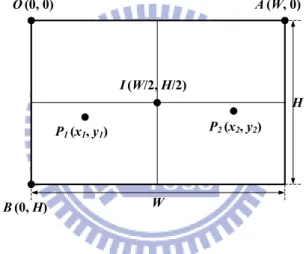
The view angle between two objects is the angular extend between them. In this section, we derive a formula to calculate the view angle between objects in an image. Figure 3.2

illustrates the coordinate layout of an image. The size of the image is W × H, and the

W H P1 (x1, y1) P2(x2, y2) I (W/2, H/2) A (W, 0) O (0, 0) B (0, H)

Figure 3.2: The coordinate layout of an image.

diagonal of the image is √W2_{+ H}2_{. Assume there is a coordinate system whose origin is}

located at the upper-left corner of the image. The upper-right corner, denoted as A, is with coordinate (W, 0), the lower-left corner, denoted as B, is with coordinate (0, H), and the

center of the image, denoted as I, is with coordinate (W/2, H/2). Let fEF L be the EFL as

taking this image. If there are two objects located at P1 and P2, we would like to develop

respectively, in the scaled one in which √W2_{+ H}2 _{= D}

135. In addition, the lens center,

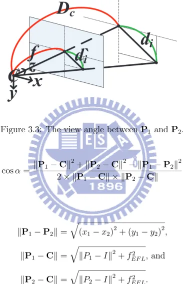
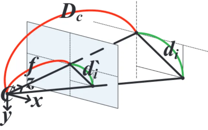
denoted as C, is with coordinate (W/2, H/2, fEF L). Figure 3.3 illustrate the view angle α

between P1 and P2. According to the law of cosines, we have

D

_c

f

x

y

z

Ȼ

d

i

d

`

i

Figure 3.3: The view angle between P1 and P2.

cos α = ∥P1− C∥ 2 +∥P2− C∥2 − ∥P1− P2∥2 2× ∥P1− C∥ × ∥P2− C∥ (3.6) where ∥P1 − P2∥ = √ (x1− x2) 2 + (y1− y2) 2 , ∥P1− C∥ = √ ∥P1− I∥ 2 + f2 EF L, and ∥P2− C∥ = √ ∥P2− I∥2+ f_{EF L}2 .

Then, α can be obtained from Eq. (3.7)

α = arccos ( ∥P1− C∥2+∥P2− C∥2− ∥P1− P2∥2 2× ∥P1− C∥ × ∥P2− C∥ ) . (3.7)

3.3

Geometry between Camera and Objects

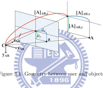
Geometry defines the relation of camera and objects with coordinate systems between them. In this section, we introduce the coordinate systems that exist in camera and objects and the projection relation between them. Coordinate systems include Earth frame and AR frame as illustrated in Fig. 3.4. A [A]AR,x a ax xAR C [A]AR,z [A]AR,y ay f zAR yAR

Figure 3.4: Geometry between user and objects

Earth frame is used in tracking objects moving on the ground. BE _={bE

1, bE2, bE3} is a

base of the Earth frame in which                bE

1 is the unit vector pointing to the north

bE₂ is the unit vector pointing to the east

bE

3 is the unit vector pointing to the ground perpendicularly

The locations of POI stored in database and the camera we want to find are defined in Earth frame. AR frame is related to the smartphone display. We assume the device is held horizontally, the screen is facing the user, and the button is at the right. Axis x, y and z

of the AR frame in which                bAR

1 is the along the x-axis of the screen (right)

bAR

2 is the along the y-axis of the screen (down)

bAR₃ is the along the direction of the lens (front)

C, the center of the lens, is the origin of the AR frame. f is the virtual focal length (if

the screen is considered as a film). If an object is far from the lens, the distance from the lens to the image is roughly equal to f . If we place the screen in front of the lens at the distance of f , then a projection relation exists between objects and images. Let

C′ denote the center of the screen,

a denote an object, and

a′ denote the image of the object.

We have C′ =         0 0 f         AR ,a =         ax ay az         E and a′ =         ax′ ay′ f         AR .

We have [a]AR = TE→AR([a]E−[C]E) where TE→ARis the rotation matrices from E-frame

to AR-frame. Since Ca′ ∥ Ca, similar relation is inferred in Eq. 3.8.

Chapter 4

AR-based Positioning

In this chapter, two AR-P problem are defined according to the view angle and geometry between user and objects and two AR-P algorithm, View Angle and Similar Triangle algo-rithm, are used to solve these problems alternately. In Fig. 4.1 taken by built-in camera in handheld device, there are several POIs whose coordinates are known, and the view an-gles and geometry between user and POIs can be obtained by drag-and-drop related AR objects on the screen of handheld device.The positioning problem raised here is to find the

position of the camera where the photo was taken. Let P OI = {P1, P2,· · · , Pn} denote the set of POIs with coordinates Pi(xi, yi, zi) for i = 1, 2,· · · , n, poi = {p1, p2,· · · , pn} denote the set of POIs in the image with coordinates pi(xi, yi, zi) for i = 1, 2,· · · , n, and

Angle = {Aij | Aij is the view angle between Pi and Pj} denote the set of view angles

be-tween POIs. We would like to find the location C where the image was taken.

4.1

View Angle Algorithm

The AR-P view angle problem is defined in Problem 1.

Problem 1 AR-based Positioning Problem-View Angle Input

P OI ={P1, P2,· · · , Pn}: a location set.

Angle ={Aij | ∀1 ≤ i < j ≤ n}: a view angle set.

Output

Find C (x, y, z) such that ∀1 ≤ i < j ≤ n,

Aij =]PiCPj.

According to the law of cosines, we can have the following equation system

∀Aij ∈ Angle, (4.1) ∥Pi− Pj∥ 2 =∥Pi− C∥ 2 +∥Pj− C∥ 2 − 2 ∥Pi− C∥ ∥Pj − C∥ cos Aij.

It is not easy to give a close form of C for the equation system. Moreover, if the input data are with measurement errors, it is possible that no exact solutions may exist. We propose a gradient method to solve the problem.

4.1.1

The Proposed Gradient Algorithm

Let F (x, y, z) be an evaluation function. Ideally, F (x, y, z) decreases as (x, y, z) approaching

to C, and especially, F (C) = 0. Given an initial point C0(x0, y0, z0), the gradient algorithms

recursively find a sequence of points C1, C2,· · · to approximate C such that F (Ci) decreases

and Ci goes to C. Let ▽F (x, y, z) = (∂F_∂x,∂F_∂y,∂F_∂z) denote the gradient of F (x, y, z).

Tradi-tionally, for all i≥ 0, Ci+1= Ci− △Si· ∇F (Ci) where △Si > 0 is a scalar to tune how fast

Ci approaches C. The gradient algorithm is given in Algorithm 2.

Algorithm 2 A Gradient Algorithm

Given F , C0, δ and ε i := 0 repeat Decide △Si Ci+1:= Ci− △Si· ∇F (Ci) i := i + 1 until∥Ci− Ci−1∥ < δ or |F (Ci)− F (Ci−1)| < ε

There are many possible alternatives of the evaluation function for using in the gradient algorithm. The one used in our implementation is given in Eq.4.2. A major drawback of the

F (C = (x, y, z)) = ∑ Aij∈Angle     ∥Pi− Pj∥ −     ∥Pi− C∥ 2 +∥Pj− C∥ 2 −2 ∥Pi− C∥ ∥Pj− C∥ cos Aij     1/2     2 (4.2) gradient method is the local minima problem. The evaluation function F (x, y, z) is not so perfect that there may exist local minima. The recursive algorithm may converge to a local minima instead of the real answer.

4.2

Similar Triangle Algorithm

The AR-P geometry problem is defined in Problem 3.

Problem 3 AR-based Positioning Problem-Geometry Input

P OI ={P1, P2,· · · , Pn}: a location set.

poi ={p1, p2,· · · , pn}: a image set of P OI.

Output

Find C (x, y, z) such that ∀1 ≤ i ≤ n,

PiCx : piCx= PiCy : piCy = PiCz : piCz

In this problem, we are going to find [C]E based on a and a′. The idea of Similar Triangle

algorithm as following, in Eq 3.8, we can obtain two equalities from the relation as

a′_x

a′_y [a]_AR,y =

f

[a]_AR,z (4.4)

So, one POI can provide two equations. Depending on the availability of TE→AR, we

may have three cases.

1.1 TE→AR can be obtained from the readings of the g-sensor and m-sensor. Let g and

m denote the readings of the g-sensor and m-sensor respectively.

        1 0 0 0 1 0 0 0 1         = TS→E [ m |m| |m×g|m×g −|g|g ] (4.5)

1.2 Assume m points to the north but with inclination.         1 0 0 0 1 0 0 0 1         = TS→E [ g×(m×g) |g×(m×g)| |m×g|m×g −|g|g ] (4.6)

Note that the sensor frame is not the same as the AR frame, currently we have

TS→AR=         0 −1 0 −1 0 0 0 0 −1         (4.7)

In the both cases (1.1 and 1.2), since TAR→E is known, the only unknown variable in the

system is C =         Cx Cy C         (4.8)

So, two POIs are enough to solve the linear system.

2. If TAR→E is unknown, we also need to find the rotation matrix, too. (This may be

the case in which m and g are both unknown or only m is unknown.) Although TAR→E is

a 3× 3 matrix, it can be characterized by 3 variables. So, totally 6 unknowns are in this

system. We need at least 3 POIs to find TAR→E and C. Note that the system is not linear.

Least square fitting can be used, if the equations are linear. Else these equations can be solve by numerical method such as gradient algorithm.

4.3

Implementation Issues

At least two practical issues must be solved to make the proposed AR-P algorithm feasible. First, how can we obtain the location information of the POIs in the real world? Second, how can we learn the view angle or geometry between user and POIs? To answer these two questions, we first need to give our application scenario. In the scenario, there is a POI database. Based on a coarse position information, users can query the database to find out nearby POIs and their locations.

The AR device can roughly know the current position and even orientation. The user takes a picture, and then based on the coarse position information, some AR objects of nearby POIs are displayed on the screen. If the user recognizes some POIs, he drags the AR objects and drops them at the places of the corresponding images of the POIs.

The location information of the AR objects in the real world can be known by querying the POI database. So, the first question is answered. At the same time, according to the

places where the AR objects are dropped, the coordinates of the POIs in the image are also known. Therefore, if the focal length is known, the view angles or geometry between user and POIs can be obtained by applying Eq. (3.7) or Eq. (3.8). So, the second question is also solved. However, the problems here are that we do not know the focal length. These two issues can be solved by applying the gradient algorithm or the geometry algorithm to find an effective focal length. Note that instead of the traditional EFL, the effective focal length here is proportional to the size of the LCD touch screen.

In the process, we take a picture which contains several reference POIs from a place whose coordinate in the real world is known. Applying the drag-and-drop technique, we can learn the coordinates of the POIs in the real world and also in the image. The view angles and geometry between user and POIs can be obtained from the coordinates of the POIs in the real world and coordinate of the place where the picture is taken. The inputs of the View Angle algorithm are the coordinates of the POIs in the image and the view angles between the POIs. The inputs of the Similar Triangle algorithm are the coordinates of the POIs in the image and real world. These output will be the coordinate of the center of the lens. The effective focal length is the distance between the center of the touch screen and the center of the lens.

Chapter 5

Experiment

5.1

Effective Focal Length (EFL) Experiment

A reasonable and reliable EFL is a key role of proposed positioning algorithm as discussed in previous chapter. Since the size of CCD is unknown, we need to estimate or calculate the EFL by ourselves. Two EFL experiments at different places are designed to View Angle and Similar Triangle algorithm alternately in the following. In both EFL experiments, the

camera, i.e., the AR device, is an HTC Desire smartphone that is equipped with a 480× 800

pixels LCD touch screen and a camera. The camera is with a variable-focal-length lens. However, in the experiments, the focal length is fixed. Positioning effect of focal lengths is analyzed in 5.2.

5.1.1

EFL Experiment of View Angle Algorithm

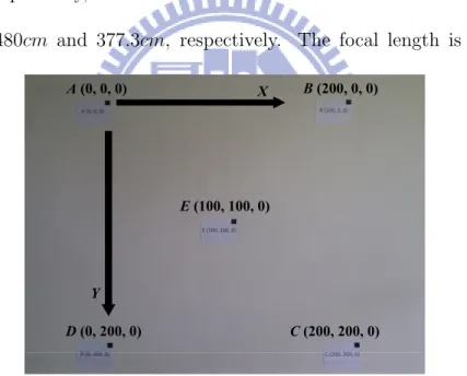
In our experiments, 5 points A, B, C, D and E are marked on a flat wall as illustrated in

Figure 5.1. A coordinate system in which A is the origin, −→AB is the x-axis,−−→AD is the y-axis,

and the z-axis points outward, is setup. Note that the coordinate system does not follow the right hand rule. The coordinates of A, B, C, D and E in the coordinate system are (0, 0, 0), (200, 0, 0), (200, 200, 0), (0, 200, 0) and (100, 100, 0), respectively. We take 3 pictures, named Pic1, Pic2, and Pic3, from 3 different places, including (100, 100, 320), (100, 100, 480) and

(−100, 100, 320), respectively, and all are with centers at E. The distances from the camera

to E are 320cm, 480cm and 377.3cm, respectively. The focal length is recorded by AR

X Y A (0, 0, 0) B (200, 0, 0) C (200, 200, 0) D (0, 200, 0) E (100, 100, 0)

Figure 5.1: The coordinates and arrangement of A, B, C, D and E.

devices in the picture file. In the following discussion, we use A, B, C, D and E to denote the markers and also their coordinates in the real world, and A, B, C, D and E to denote the image of the markers and also their coordinates in the image.

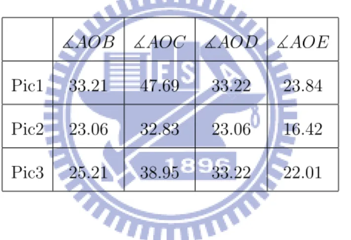
First, we verify the proposed algorithm by calculating the EFL of the AR device. To calculate the EFL, we adopt Algorithm 2 by inputting the coordinates of A, B, C, D and E (in the image coordinate) and view angles between A, B, C, D and E calculated from the real world coordinates to estimate the coordinate of the lens center in the image coordinate. Then, the EFL can be given by calculating the distance between the lens center and the picture center. Table 5.1 gives the view angles between objects that are calculated from the real world coordinate. Table 5.2 gives the coordinates of A, B, C, D and E in the image

Table 5.1: The view angles between objects (in degrees). ]AOB ]AOC ]AOD ]AOE

Pic1 33.21 47.69 33.22 23.84

Pic2 23.06 32.83 23.06 16.42

Pic3 25.21 38.95 33.22 22.01

coordinate. Table 5.3 gives the estimated EFL in cm. We can see that the EFL calculated from Pic1 is larger than the EFL calculated from Pic2. This is due to the focal length here actually is the image distance. Pic1 has a smaller object distance, and thus has a larger image length. In average, the focal length is 7.69cm.

5.1.2

EFL Experiment of Similar Triangle Algorithm

Table 5.2: The coordinates (in cm) of A, B, C, D and E in the images.

A B C D E

Pic1 (1.661, 0.562, 0) (6.471, 0.547, 0) (6.634, 5.420, 0) (1.712, 5.431, 0) (4.180, 2.938, 0)

Pic2 (2.495, 1.525, 0) (5.636, 1.520, 0) (5.693, 4.706, 0) (2.482, 4.694, 0) (4.117, 3.075, 0)

Pic3 (2.107, 0.591, 0) (5.626, 1.090, 0) (5.773, 4.674, 0) (2.278, 5.315, 0) (4.229, 2.887, 0)

Table 5.3: The EFL (in cm) calculated based on different reference point sets.

ABC ABE ABCD ABCE ABCDE

Pic1 7.790 7.651 7.787 7.769 7.787

Pic2 7.614 7.515 7.620 7.599 7.620

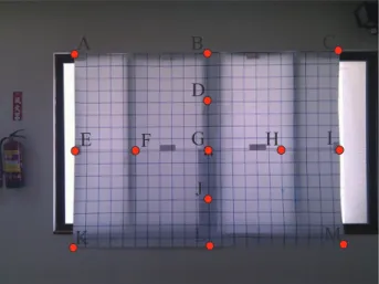
A B C D E F G H I K J M L

Figure 5.2: Test lines of experiment

poster from 3m to 17m with unit interval in one meter and all are with centers at G. EFL

is calculated by the relation of similar triangles as illustrated in Fig. 5.3. di represents the

physical length of each test line in cm. The index of test lines is i. d′_i means pixel length of

each test line on each picture which we have taken. The distance between camera and poster

is called camera distance in cm, denoted as Dc. The effective focal length is f . Using the

relation of similar triangles, we get equation f : Dc= (d′i×r) : di , where r is the pixel-to-cm

ration. By transposition, Eq. 5.1 is gotten. 8-by-4.8 cm is the physical size of HTC desire screen, and the picture size is 1024-by-768. The scales of screen and picture are different. Considering the problem of distortion of picture, we use the scale of picture as the major scale size. A virtual screen is made by resizing the 8-by-4.8 cm to 8-by-6 cm. Each picture we take are resized from 1024-by-768 to 800-by-600 pixels. The pixel-to-cm ratio r of each

picture can be calculated by 8/800 = 0.01 cm/pixel. The Dc, di and d′i are known, and then

where AK, KM, . . . , T REN D is the test line of experiment illustrated in Fig. 5.2.

D

_c

f

x

y

z

Ȼ

d

_i

d

`

_i

Figure 5.3: Similar triangles relation among camera and POIs

f = Dc× (d

′

i× r)

di

(5.1)

3 main analysis cases are focused in the following:

• Camera distance Dc vs. EFL f

• Physical length of test lines vs. EFL f • Overall variant of EFL f

a. Camera distance Dc vs. EFL f According to Fig. 5.4, trend line T REN D of EFL

f is descending as Dc is increasing. It converges to real focal length on the increase of Dcas

Eq. 3.1.

7.4 7.5 7.6 7.7 7.8 7.9 8 8.1 3 0 0 4 0 0 5 0 0 600 700 800 900 1000 1100 1200 1300 1400 1500 1600 1700 F oc al L e n gt h (c e n ti m e te r) Distance (centimeter) AK KM CM AC EI BL AM CK AVG TREND Test Line

Figure 5.4: The effective focal length with different camera distance Dc

of EFL ∆f is affected by _d1

i for each finger touch error ∆d

′

i, considering Dc is fixed. The

1

di of longer test lines is smaller than the ones of short test lines. Fig. 5.5 illustrates the

experiment result. Test lines EI and BL are longer test lines in Fig. 5.2; test lines F H and DJ are shorter ones. F H and DJ have more variance than the result of EI and BL.

7.3 7.4 7.5 7.6 7.7 7.8 7.9 8 300 40 0 500 60 0 700 80 0 900 1 0 0 0 1 1 0 0 1 2 0 0 1 3 0 0 1 4 0 0 1 5 0 0 1 6 0 0 1 7 0 0 F o c a l L e n g th ( c e n ti m e te r) Distance (centimeter) EI BL FH DJ Test Line

Figure 5.5: Long line and short Line

c. Overall variant of EFL f It shows average, standard deviation and trend line of EFL f in Fig. 5.6. According to average line AV G, the EFL f is in inverse proportion to the

proportion to Dc because the pixel length d′i is in inverse proportion to Dc. It causes the

possibility of measurement error to be increased. If the measurement error εdi of each test

line is the same, and then longer physical test lines have smaller error of EFL f than the one that shorter test lines have.

7.3 7.4 7.5 7.6 7.7 7.8 7.9 8 8.1 300 500 700 900 1100 1300 1500 1700 F oc al L e n gt h ( ce n ti m e te r) Distance (centimeter) AVG TREND

Figure 5.6: Average testing focal length and trend line and trend line

The EFL f converges as the increase of camera distance Dc. The standard deviation of

EFL f will increase when Dc is larger than 9m. According to Fig. 5.6, the most suitable

Dc is between 5m and 9m. We shall select POIs within this range and select POI set with

5.2

AR-P Experimental Results

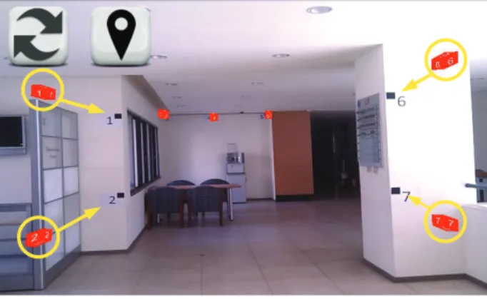
In our experiments, the positioning effect factors of proposed positioning algorithms, View Angle and Similar Triangle algorithm, are analyzed according to combinations of AR objects, user’s location and the effective focal length that is the result of section 5.1. The proposed positioning algorithms are tested at 7 locations with 7 POIs. 7 test locations and 7 POIs are distributed on the second floor of a building as illustrated in Fig. 5.7, where blue points 1, 2 . . . and 7 are the test locations and red points 1, 2 . . . and 7 are the POIs known in databases. Test locations are distributed according to distances. There is one meter between each test location. POIs are marked on flat walls according to distance, height and plane as illustrated in Fig. 5.8, where numbers, located on the walls, represented the POIs and black blocks are used to match the AR objects. A coordinate system in which test location 4 is the origin, the east of Earth’s magnetic field is the x-axis, North Magnetic Pole is the y-axis and z-axis points to sky, is setup.

1,2 ₃ 4 5 6,7 1 2 3 4 5 6 7

Figure 5.7: Experiment locations in map

6 (175, 645, 216) 7 (175, 645, 108) 3 (-93, 1400, 270) 5 (175, 1400, 270) Z Y X 2 (-92, 830, 96) 4 (35, 1400, 270) 1 (-92, 830, 216)

Figure 5.8: AR-P experiment environment

Fig. 5.9 illustrates the system interface. Red cubes are AR objects used to match the POIs. The number in AR objects represents its POI number. The first button on the upper left side is refresh button used to return the type of taking picture; positioning button located the second button is used to perform AR-P algorithm to position.

Since the positioning effects of focal lengths calculated by different focal length exper-iments are still unknown, we need to compare or verify them with different focal lengths.

Proposed positioning algorithms are performed according to ranges of focal length from 7.5cm to 8.5cm, and unit interval is 0.1cm. 7.76cm of average focal length has the smallest positioning error in the positioning result of View Angle algorithm as illustrated in Fig. 5.9, where line 1, 2, ..., 7 represent test position 1, 2, ..., 7, and the average focal length of previous focal length experiment of View Angle algorithm is 7.69cm. There are closed positioning errors between focal length 7.76cm and 7.69cm in Fig. 5.9, so we use 7.69cm as the focal length in View Angle algorithm. Fig. 5.10 gives the positioning result of Similar Triangle algorithm, where line 1, 2, ..., 7 represent test position 1, 2, ..., 7. Compared with focal length converged in range from 7.5cm to 7.65cm of previous focal length experiment of Similar Triangle algorithm, focal length 8.08cm has the smallest positioning error. Since there are a gap of positioning error between focal length calculated by previous focal length experiment of Similar Triangle algorithm and focal length 8.08cm, we use focal length 8.08cm as the focal length in Similar Triangle algorithm.

0 50 100 150 200 250 7.5 7.6 7.7 7.8 7.9 8 8.1 8.2 8.3 8.4 8.5 P os it ion in g E rr or (c m ) Focal Length 1 2 3 4 5 6 7 Test Loc.

Figure 5.9: View Angle algorithm result: positioning error affected by focal length

dis-0 20 40 60 80 100 120 140 7.5 7.6 7.7 7.8 7.9 8 8.1 8.2 8.3 8.4 8.5 P os it ion E rr or (c m ) Focal Length 1 2 3 4 5 6 7 Test Loc.

Figure 5.10: Similar Triangle algorithm result: positioning error affected by focal length tances, where “VAGIG” represents ”View Angle Good Initial Guess” that means the View Angle algorithm with initial point (0, 0, 0), “VABIG” represents ”View Angle Bad Initial

Guess” that means the View Angle algorithm with initial point (−500, −500, −500) and

“ST” is the Similar Triangle algorithm. Fig. 5.12 illustrates the positioning result of pro-posed algorithm according to the POI combination numbers. The problems of local minima exist in View Angle algorithm. Average positioning error of View Angle algorithm is 88.9cm when selecting the better initial point, but 245.95cm in poor initial points. Similar Triangle algorithm has the 74.34cm of average positioning error.

Experiment Analysis

In this section, position effect factors that may affect the accuracy of the proposed positioning algorithm are analyzed. These factors include the initial point, combinations of AR objects, user’s locations and focal lengths. To reach the highly accuracy positioning result, we show how to select these factors. Finally, the positioning results of View Angle and Similar Triangle

0 50 100 150 200 250 300 350 1 2 3 4 5 6 7 P os it ion in g E rr or (c m ) Test Location VAGIG VABIG ST

Figure 5.11: Average positioning results with different test locations

Combination Numbers D is ta n ce E rr o r( cm ) 0 100 200 300 400 500 600 700 800 900 1000 2 3 4 5 6 7 ST VAGIG VABIG

Figure 5.12: Positioning result affected by combinations number algorithm are compared.

View Angle algorithm

Local minima: The existence of local minima of the evaluation function is an inevitable problem. This problem could be alleviated when the POI number we picked is more. To

blue points represent the local minima, read points means POIs and the real locations is green point. From the result, poor initial point converged to local minima easily when POI numbers we picked is few and difficultly when POI numbers we picked is more. However, there still has change to converge to local minima even more POIs are selected. The selection of the initial point significantly affects the answer given by the View Angle algorithm.

Figure 5.13: Local minima with 3 points

Combinations of AR objects: Positioning result are affected by the combinations of AR objects due that the relation between user and AR objects provides the information of user’s location. The more combinations of AR objects we pick, the more accuracy of user’s location we get as illustrated in Fig. 5.15. Even the problem of local minima could be alleviated. 0 100 200 300 400 500 600 700 800 2 3 4 5 6 7 P os it ion in g E rr or (c m ) Combination Numbers VAGIG VABIG

Figure 5.15: View Angle algorithm: Positioning error affected by combination numbers

Combinations of AR objects are also an important factor. The near AR objects provide the closed information of user’s location. The experiment results of the POI combinations of

same plane illustrates in Fig. 5.16, where column 34 represents the combinations of P OI{3, 4}

and other columns follow this rule. POI 3, 4 and 5 are in the same plane as illustrated

in Fig. 5.8. POI combinations {3, 4}, {3, 5} and {4, 5} are nearly the same in positioning

relations and POI combinations{3, 4, 5} are the sum of those of POI combinations, therefore

POI combinations {3, 4, 5} have closed positioning result with POI combinations {3, 4},

{3, 5} and {4, 5}. Average positioning errors of those combinations are above 150cm. POI

selections of diversity. The more diversity the POI combinations have, the more information of user’s location they provide and there would have the better position results.

0 20 40 60 80 100 120 140 160 180 P os it ion in g E rr or (c m ) Combinations 3 4 3 5 4 5 3 4 5 1 5 6 2 3 7 POI Set

Figure 5.16: Positioning error affected by POI combinations of same plane

Distance between user and POI combinations would affected the position result due that the evaluation functions of View Angle algorithm are the relation of view angle between POIs and user. Tiny touch error when drag-and-drop AR objects may cause the error of view angle calculation and then the positioning error. Fig. 5.17 gives the experiment result of distant POI combinations. POI 1 and 2 are at the near plane; POI 3, 4 and 5 are at the

far plane as illustrated in Fig. 5.8. Experiment results show the POI combinations {1, 2, 7}

have better positioning result than the result of POI combinations {3, 4, 7}, {3, 5, 7} and

{4, 5, 7}. The positioning effect factor of distant POI combinations can be explained in a

simple formula as illustrated in Fig. 5.4 and 5.1 For each ∆d′_i, the positioning error ∆di is

determined by Dc

f . Under the fixed focal length, the positioning error would be worse when

Dcgoes up. The position effect factor of user’s location has the same meaning. As illustrated

0 20 40 60 80 100 120 140 160 180 P os it ion in g E rr or (c m ) Combinations 1 2 7 3 4 7 3 5 7 4 5 7 POI Set

Figure 5.17: Positioning error affected by combinations of distant POI

Similar Triangle algorithm

Combinations of AR objects: Positioning results are affected by the combinations of AR objects as previous analysis in View Angle algorithm section. Fig. 5.18 is the aver-age positioning result compared with combination numbers. Total positioning errors have significantly decreased from 112cm with 2 POIs to 48cm with 7 POIs.

0 20 40 60 80 100 120 2 3 4 5 6 7 P os it ion in g E rr or (c m ) Combination Numbers ST

Figure 5.18: Positioning result affected by POI combinations

Distances are also the positioning effect factor as View Angle algorithm Fig. 5.19 lists {1, 2} and {6, 7}

at the near plane have better positioning result than POI combinations{3, 4}, {3, 5}, {4, 5}

and {3, 4, 5} at far plane.

0 20 40 60 80 100 120 140 160 P os it ion in g E rr or (c m ) Combinations 3 4 3 5 4 5 3 4 5 1 2 6 7 POI Set

Figure 5.19: Positioning error affected by combinations of distant POI

POI combinations that POIs are closed or nearly in the same line would affect the posi-tioning result due that the similar relation is used in Similar algorithm. POI 1 and 3 and POI 5 and 6 are the examples as illustrated in Fig. 5.20. POI combinations that have POI 1 and 3 or POI 5 and 6 would have poor positioning result compared to other combinations.

0 50 100 150 200 250 300 350 P os it ion in g E rr or (c m ) Combinations 1 3 1 4 5 6 1 3 4 1 7 2 6 POI Set

Focal length: Positioning results of Similar Triangle algorithm are affected by the focal length as illustrated in the Fig. 5.10. Tiny difference of focal length would have an impact significantly in positioning result as the distance between user and POIs goes up. The scope of Similar Triangle algorithm is given in Fig. 3.4. According to the Similar Triangle algorithm, Fig. 5.21 lists 4 relation formulas between user and 2 POIs and the solution of user’s location is given in Fig. 5.22. Focal length locates at denominator in solution of x and y, and locates at numerator in solution of z. When the focal length goes up, x and y would be decreased until converge into a fixed value and z would be increased into infinity. On the inverse condition, when the focal length goes down, x and y would be increased into infinity and z would be decreased until converge into a fixed value. The effects of x, y and z is illustrated in Fig. 5.23 and Fig. 5.24 gives the experiment formula. The experiment result shows z would be increased significantly and x y decreased slightly. The focal length would affect the z value of user’s location significantly.

a′_x [a]_c,x = f [a]_c,z a′_y [a]_c,y = f [a]_c,z b′_x [b]_c,x = f [b]_c,z b′_y [b]_c,y = f [b]_c,z

Comparison of two proposed positioning algorithm: Fig. 5.11 and Fig. 5.12 com-pared the View Angle algorithm with Similar Triangle algorithm. View Angle algorithm is affected by the problems of local minima but Similar Triangle algorithm has no such prob-lems. When the combination numbers go up, positioning errors of both proposed positioning algorithms have significantly decreased. When combination numbers of proposed algorithms increase and proposed algorithms have a better initial point, the positioning result of View Angle algorithm are better than the positioning result of Similar Triangle algorithm. Gener-ally, Similar Triangle algorithm has a steady and good positioning result than the positioning result of View Angle algorithm.

From the experiment result, The focal length of View Angle algorithm is 7.69cm and 8.083cm is average focal length of Similar Triangle algorithm that have lowest average posi-tioning error. Users should avoid selecting the combinations that POIs are closed or in the same line or plane and user should be near to POIs. Compared to the View Angle algo-rithm, Similar Triangle algorithm do not have problem of local minima and have a better positioning result.

X = ( [a]_c,z− [b]_c,z) ((a′_x− b′_x) (2a′_xb′_x+ a′_yb′_y)+ a′2_yb′_x− b′2_ya′_x ) 2 (f + ∆f ) ( (a′_x− b′_x)2+(a′_y− b′_y)2 ) + ( a′_y − b′_y) ((a_y′ − b′_y) ([a]_c,x+ [b]_c,x )

−(a′_x+ b′_x) ([a]_c,y− [b]_c,y

)) 2 ( (a′_x− b′_x)2+(a′_y − b′_y)2 ) + ( a′_x− b′_x) (a′_x[b]_c,x− b′_x[a]_c,x ) (a′_x− b′_x)2+(a′_y − b′_y)2 Y = ( [a]_c,z− [b]_c,z) ((a′_y− b′_y) (2a′_yb′_y+ a′_xb′_x)+ a′2_xb′_y− b′2_xa′_y ) 2 (f + ∆f ) ( (a′_x− b′_x)2+(a′_y − b′_y)2 ) + (

a′_x− b′_x) ((a_x′ − b′_x) ([a]_c,y+ [b]_c,y ) −(a′_y + b′_y) ([a]_c,x− [b]_c,x )) 2 ( (a′_x− b′_x)2+(a′_y − b′_y)2 ) + (

a′_y− b′_y) (a′_y[b]_c,y − b′_y[a]_c,y

) (a′_x− b′_x)2+(a′_y − b′_y)2

Z =

− (f + ∆f)((a′_x− b′_x) ([a]_c,x− [b]_c,x

)

+(a′_y− b′_y) ([a]_c,y− [b]_c,y

)) (a′_x− b′_x)2+(a′_y − b′_y)2 + ( a′_x− b′_x) (a′_x[a]_c,z− b′_x[b]_c,z ) +(a′_y+ b′_y) (a′_y[a]_c,z− b′_y[b]_c,z ) (a′_x− b′_x)2+(a′_y− b′_y)2

-200 -100 0 100 200 300 400 7.5 7.6 7.7 7.8 7.9 8 P os it ion ( cm ) Focal Length x y z

Figure 5.23: The x, y, z result of test Location 1 in AR frame

               X = 240.50558_f + 17.222198 Y = 77.857063_f − 165.863 Z = f ∗ (−50.886617) + 722.35833

Chapter 6

Conclusions

Most current commercial positioning solutions could not meet the requirement of high-precision positioning for LBS application with AR. In this paper, two AR-based positioning methods, View Angle and Similar Triangle algorithm, are proposed. The average positioning error of View Angle algorithm is from 88.9cm to 245.9cm caused by the local minima issue of gradient method. The Similar Triangle algorithm does not have local minima problems and have a better average positioning error of 74.34cm. In the future work, matching POIs by hand can be replaced with automation such as vision-based or laser detection. Then, the AR-P system will be more fast, easy and accurate without human interaction. The problems of local minima of View Angle algorithm should be solved by the closed form solution or a new method to converge the solution to the global minima. Our system can be combined with feedback information routing and other positioning technique such as GPS or WiFi positioning to implement an real-time and high accuracy evacuation system.

Bibliography

[1] D. Huber, “Background positioning for mobile devices - android vs. iphone,” 2012.

[2] T. Manesis and N. Avouris, “Survey of position location techniques in mobile systems,” in Proceedings of the 7th International Conference on Human Computer Interaction with Mobile Devices and Services (MobileHCI). New York, NY, USA: ACM, Sep 2005, pp. 291–294.

[3] N. F. Krasner, “GPS receiver utilizing a communication link,” U.S. Patent

US005 841 396A.

[4] Y. Zhao, “Standardization of mobile phone positioning for 3G systems,” IEEE Com-munications Magazine, vol. 40, no. 7, pp. 108–116, Jul 2002.

[5] D. Pozar and S. Duffy, “A dual-band circularly polarized aperture-coupled stacked mi-crostrip antenna for global positioning satellite,” IEEE Transactions on Antennas and Propagation, vol. 45, no. 11, pp. 1618–1625, Nov 1997.

[6] P. Enge, T. Walter, S. Pullen, C. Kee, Y.-C. Chao, and Y.-J. Tsai, “Wide area aug-mentation of the global positioning system,” Proceedings of the IEEE, vol. 84, no. 8, pp. 1063–1088, Aug 1996.

[7] P. Bahl and V. Padmanabhan, “RADAR: an in-building rf-based user location and tracking system,” in Proceedings of the Nineteenth Annual Joint Conference of the IEEE Computer and Communications Societies (INFOCOM), Mar 2000, pp. 775–784.

[8] C.-C. Lo, L.-Y. Hsu, and Y.-C. Tseng, “Adaptive radio maps for pattern-matching localization via inter-beacon co-calibration,” Pervasive and Mobile Computing, vol. 8, no. 2, pp. 282–291, Apr 2012.

[9] C. Figuera, I. Mora-Jimenez, A. Guerrero-Curieses, J. Rojo-Alvarez, E. Everss, M. Wilby, and J. Ramos-Lopez, “Nonparametric model comparison and uncertainty evaluation for signal strength indoor location,” IEEE Transactions on Mobile Comput-ing, vol. 8, no. 9, pp. 1250–1264, Sep 2009.

[10] C.-C. Lo, J.-J. Chen, C.-Y. Yang, Y.-C. Tseng, S.-M. Huang, Y.-N. Hung, and C.-M. Tseng, “From barren to beautiful: A pattern-matching localization scheme integrat-ing heterogeneous network data,” in The 13th Asia-Pacific Network Operations and Management Symposium (APNOMS), Sep 2011.

[11] T. Caudell and D. Mizell, “Augmented reality: an application of heads-up display technology to manual manufacturing processes,” in Proceedings of the Twenty-Fifth

[12] T.-H. Wang, M.-C. Lu, W.-Y. Wang, and C.-Y. Tsai, “Distance measurement using single non-metric CCD camera,” in Proceedings of the 7th WSEAS International Con-ference on Signal Processing, Computational Geometry and Artificial Vision (ISCGAV). Stevens Point, Wisconsin, USA: World Scientific and Engineering Academy and Society (WSEAS), Aug 2007, pp. 1–6.

[13] C.-C. Chen, M.-C. Lu, C.-T. Chuang, and C.-P. Tsai, “Outdoor image recording and area measurement system,” in Proceedings of the 7th WSEAS International Confer-ence on Signal Processing, Computational Geometry and Artificial Vision (ISCGAV). Stevens Point, Wisconsin, USA: World Scientific and Engineering Academy and Society (WSEAS), Aug 2007, pp. 129–134.

[14] ——, “Vision-based distance and area measurement system,” WSEAS Transactions on Signal Processing, vol. 4, no. 2, pp. 36–43, Feb 2008.

[15] M.-C. Lu, W.-Y. Wang, C.-C. Chen, and C.-P. Tsai, “Nighttime vehicle distance alarm system,” in Proceedings of the 7th WSEAS International Conference on Signal

Pro-cessing, Computational Geometry and Artificial Vision (ISCGAV). Stevens Point,

Wisconsin, USA: World Scientific and Engineering Academy and Society (WSEAS), Aug 2007, pp. 226–230.

[16] D. Braganza, D. Dawson, and T. Hughes, “Euclidean position estimation of static fea-tures using a moving camera with known velocities,” in Proceedings of the 46th IEEE Conference on Decision and Control, Dec 2007, pp. 2695–2700.

[17] T. Luhmann, “Precision potential of photogrammetric 6DOF pose estimation with a single camera,” ISPRS Journal of Photogrammetry and Remote Sensing, vol. 64, no. 3, pp. 275–284, May 2009.

[18] X. Li, J. Wang, A. Olesk, N. Knight, and W. Ding, “Indoor positioning within a single camera and 3d maps,” in Ubiquitous Positioning Indoor Navigation and Location Based Service (UPINLBS), Oct 2010.

[19] A. Ryberg, A.-K. Christiansson, and K. Eriksson, “Accuracy investigation of a vision based system for pose measurements,” in The 9th International Conference on Control, Automation, Robotics and Vision, Dec 2006.

[20] J. Kim and H. Jun, “Vision-based location positioning using augmented reality for indoor navigation,” IEEE Transactions on Consumer Electronics, vol. 54, no. 3, pp. 954–962, Aug 2008.

[21] L. C. Huey, P. Sebastian, and M. Drieberg, “Augmented reality based indoor positioning navigation tool,” in IEEE Conference on Open Systems (ICOS), Sep 2011, pp. 256–260.

[22] Y. Nakazato, M. Kanbara, and N. Yokoya, “Wearable augmented reality system using invisible visual markers and an IR camera,” in Proceedings of the Ninth IEEE Interna-tional Symposium on Wearable Computers, Oct 2005, pp. 198–199.

[23] H. Hile and G. Borriello, “Positioning and orientation in indoor environments using camera phones,” IEEE Computer Graphics and Applications, vol. 28, no. 4, pp. 32–39,

[24] A. Comport, E. Marchand, M. Pressigout, and F. Chaumette, “Real-time markerless tracking for augmented reality: the virtual visual servoing framework,” IEEE Trans-actions on Visualization and Computer Graphics, vol. 12, no. 4, pp. 615–628, Jul-Aug 2006.

[25] Y.-C. Chiu and P. Mirchandani, “Online behavior-robust feedback information routing strategy for mass evacuation,” IEEE Transactions on Intelligent Transportation Sys-tems, vol. 9, no. 2, pp. 264–274, Jun 2008.

[26] C.-Y. J. Lin, Y.-C. Tseng, and C.-W. Yi, “Pear: personal evacuation and rescue sys-tem,” in Proceedings of the 6th ACM Workshop on Wireless Multimedia Networking