Electronic cam motion generation with special reference to constrained velocity, acceleration, and jerk

Abstract

Electronic cam motion involves velocity tracking control of the master motor and trajectory generation of the slave motor. Special concerns such as the limits of the velocity, acceleration, and jerk are beyond the considerations in the conventional electronic cam motion control. This study proposes the curve-fitting of a Lagrange polynomial to the cam profile, based on trajectory optimization by cubic B-spline interpolation. The proposed algorithms may yield a higher tracking precision than the conventional master-slaves control method does, providing an optimization problem is concerned. The optimization problem contains three dynamic constraints including velocity, acceleration, and jerk of the motor system. © 2004 ISA—The Instrumentation, Systems, and Automation Society.

Keywords: Electronic cam; Tracking control; Trajectory generation; Trajectory optimization; Master-slaves

1. Introduction

In this study, the electronic cam 共ECAM兲 mo-tion is generated in two stages, the first of which is a typical electronic gearing process which is fo-cused on the velocity tracking control of the mas-ter motor. Steven 关1兴 specified a tracking control electronic gearing system called an ‘‘optimal feed-forward tracking controller,’’ concerned primarily with the design of the slave controller. However, he did not consider the output properties of the master motor, including the measurement noise, periodic errors, and external harmonic distur-bances. In practice, the measurement noise or the external disturbance must be controlled and elimi-nated by modeling the disturbances, before apply-ing trackapply-ing control to estimate the master posi-tion. This paper proposes the use of a disturbance estimator 关2兴 to suppress the external disturbance.

The design of this disturbance estimator is practi-cal and easy to implement.

This approach to obtaining a highly precise estimate of the master position involves Nth-order polynomial tracking. For example, the fifth-order polynomial estimate is more precise than the third-order polynomial estimation by a factor of about 10 000. The advantage of the proposed tracking method is that the low-frequency harmonic disturbances of a loaded master are very precisely estimated. Such nominal harmonic disturbances are observed in many industrial applications 关3兴. In practice, the frequencies of the external disturbances are expected to be far below the Nyquist frequency 关4兴 of the real-time system.

ECAM motion regulates the slave motion to fol-low a predetermined trajectory, which is a function of the position of the master axis 关5,6兴. A cam

trajectory is generally specified by a cam profile table, which lists a set of reciprocal coordinates. Chen 关7兴 applied B-spline 关8,9兴 and polynomial curve-fitting methods to generate a smooth cam profile curve function. Kim and Tsao 关10兴 devel-oped an electrohydraulic servo actuator for use in electronic cam motion generation, and obtained improved performance. However, some original performance limits, including velocity, accelera-tion, or jerk constraints, must be considered be-cause motors have the lower loaded capacity rela-tive to the hydraulic actuators. For example, for a highly precise machining tool, chattering must be avoided, so jerking in motion must be reduced.

This study proposes an optimization algorithm 关11兴 to prevent extremely high velocities, accelera-tion, or jerk, yielding smooth motion of the slave motor without loss of precision. The proposed tracking method presented here was experimen-tally verified using a real-time program to realize the ECAM control system. The master’s system uses a disturbance estimator to eliminate external disturbances. This estimator is the prerequisite for the Nth-order polynomial tracking control. Lagrange polynomial 关9兴 curve-fitting, cubic B-spline 关9兴 interpolation and a constrained opti-mization algorithm are used to determine the po-sition of the slaves. Consequently, a tradeoff may exist between precision and constraints, which are imposed in given order of priority.

2. Prerequisite of electronic cam „ECAM… tracking control

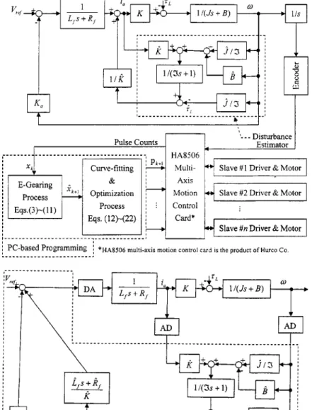
Electronic cam 共ECAM兲 control is a well-known master-slaves system. Fig. 1共a兲 schemati-cally depicts the mathematical model of the pro-posed electronic cam system. The variables and symbols in the figure are defined in the following sections. In Fig. 1共a兲, the motion of the slave mo-tor clearly depends on the estimated slave position command, p_k⫹1, which is generated by cubic B-spline interpolation, combined with an optimi-zation algorithm. Such optimioptimi-zation is performed to meet the demands of limited performance—the constraints of velocity, acceleration, and jerk. The method of cubic B-spline curve-fitting is based on substituting the estimated master position into the cam trajectory. It is established using Lagrange’s interpolation formula to generate a Lagrange

poly-nomial curve. However, the predicted master po-sition is estimated by the electronic gearing 共E-gearing兲 process.

2.1. External disturbance estimator

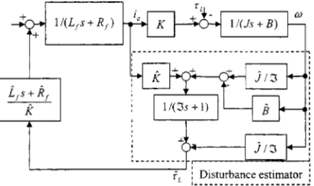
External disturbances 共or loads兲 applied to the master may directly impact the efficiency of E-gearing. Therefore disturbances must be sup-pressed. A mathematical model of the disturbance estimator, depicted in Fig. 1共a兲, is used to estimate and suppress the external loads of the master mo-tor. Fig. 1共b兲 is one practical embodiment for the proposed disturbance suppressed control.

In Fig. 1共b兲, the external load ␶L is estimated

from the input current ia and the angular velocity ␻, where K_a, Lˆ_f, Rˆ_f, Kˆ , Jˆ, andBˆ represent the nominal back electromotive force constant, the nominal armature current inductance, the nominal armature current resistance, the nominal torque constant, the nominal moment of inertia, and the nominal damping coefficient of the motor, respec-tively. Furthermore, V_{re f}, L_f, R_f, K, J, and B represent the reference voltage input, the actual armature current inductance, the actual armature current resistance, the actual 共uncertain兲 torque constant, the actual 共uncertain兲 moment of inertia, and the actual 共uncertain兲 damping coefficient of the motor, respectively. Consider the dynamics of a typical dc motor:

Jˆ␻˙⫹Bˆ␻⫹␶L⫽Kˆ•ia⇒␶L⫽Kˆ•ia⫺Jˆ␻˙⫺Bˆ␻. 共1兲

According to Fig. 2共a兲, this estimator cannot be realized because of the differential term (Jˆs) of angular velocity. The estimator depicted in Fig. 2共a兲 is also very numerically sensitive to the mea-surement noise because it yields high gains in the high-frequency field. Accordingly, a first-order low-pass filter is used to estimate the disturbance

␶ˆL, as shown in Fig. 2共b兲, where ␶ˆL⫽ 1 共Is⫹1兲␶L 共2兲 and ␶ˆL ␻ ⫽ ⫺共Jˆs⫹B兲 Is⫹1 ⫽⫺ Jˆ I ⫹ ⫺Bˆ⫹Jˆ/I Is⫹1 . 共3兲

Rearranging this external disturbance estimator in Fig. 3 yields no differential term. The estimated

disturbance (␶ˆL) is then fed back to the current

loop, and the external disturbance is suppressed. In practice, due to the current loop’s bandwidth being much larger than the speed loop’s band-width, the electrical dynamic response 关1/(Lfs ⫹Rf)兴 may be ignored from the model of Fig.

1共b兲.

2.2. Suppressing external disturbance

According to Fig. 3, the pole of the disturbance estimator equals the pole of the low-pass filter,

specified by Eq. 共2兲. Thus the estimated value for low delay time is obtained by reducing the time constant 共I兲 of the low-pass filter. However, the small time constant trades off the estimated preci-sion and robustness because it suffers more on measurement noise and modeling uncertainty.

Fig. 2共b兲 is equivalently transformed to Fig. 2共c兲 to elucidate the effect of the external disturbance

(␶L). According to Fig. 2共c兲, the effect of ␶L is

that of passing ␶L through the filter Is/(Is⫹1).

Accordingly, the external disturbance can be sup-pressed when the disturbance frequency is less

Fig. 1. 共a兲 Mathematical model of the proposed electronic cam system. 共b兲 Block diagram of the proposed disturbance estimator for one practical embodiment.

than 1/I rad/s. Thus the smaller time constant I yields better efficiency for suppressing high-frequency disturbances. However, a tradeoff exists between estimated precision and robustness, as de-scribed in the above paragraph.

Due to considerations of robustness, the mea-surement noise and the modeling uncertainty must also be considered in determining the time con-stant I. The Appendix discusses the sensitivities, S_KGc_{, S}

J

Gc_{, andS}

B

Gc_{to the uncertainties, whereS}

K Gc_, S_JGc_{, and S}

B

Gc _{are the sensitivities of the current} loop transfer function G_c to the uncertain param-eters K, J, and B, respectively. Moreover, the ef-fect of measurement noise is discussed with refer-ence to a numerical simulation in Section 5.1.

3. Electronic gearing„E-gearing… process The electronic gearing共E-gearing兲 differentiates itself from the mechanical gearing because the

E-gearing system employs only electronic means to achieve the constant input/output velocity ratio. It is assumed that the output velocity control sys-tem is stiff and the main issue for the electronic E-gearing is to predict the future master velocity from its past. The velocity of the slave 共output兲 motor is controlled according to the velocity of the master 共input兲 motor.

The velocity of the master motor varies when loads or other external disturbances are applied. Therefore the master velocity is not usually con-stant and may exhibit harmonics. Even though the amplitudes of the harmonic velocity are greatly reduced by using the proposed disturbance estima-tor, there still exists velocity variations. The pro-cedure for estimating the master position and/or velocity is an important step for E-gearing. Meth-ods of tracking control have been developed in various fields, and include radar tracking control and others关12兴. This study proposes an Nth-order polynomial tracking method to perform the E-gearing process.

According to the Nth-order polynomial, the master velocity at time t can be expressed as

␻⫽

兺

i⫽0 N

c_iti_{. 共4兲}

To determine the above coefficients

(c0,c1,...,cN) in real time, two procedures are

proposed.

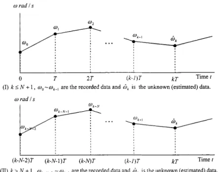
共i兲 The initial procedure, t⫽kT, 1⭐k⭐N⫹1, is the various order 关(k⫺1)th order兴 polynomial extrapolation, where the symbol k is a real-time counter of time base, T is the PC-based program-ming sampling time, and kT denotes the present time over all this paper,

Fig. 2. The estimation of external disturbance.

Fig. 3. The external disturbance estimator and external dis-turbance eliminated control.共i兲 k⭐N⫹1,␻0⬃␻k⫺1are the

recorded data and␻ˆkis the unknown共estimated兲 data. 共ii兲

k⬎N⫹1,␻k⫺N⫺2⬃␻k⫺1 are the recorded data and␻ˆk is the unknown共estimated兲 data.

兺

c_i共l•T兲i_⫽␻

l, l⫽0 to k⫺1. 共5兲

Here we use the assumption of00⫽1.

共ii兲 The main procedure, t⫽kT, k⬎N⫹1, is the fixed Nth-order polynomial extrapolation:

兺

Similarly, the symbol k is a real-time counter of time base, T is the PC-based programming sam-pling time. Where ␻_l关⫽(x_l⫹1⫺x_l)/T兴 are the

measured angular velocities during the interval 关lT,(l⫹1)T兴, x_l are the recorded positions of the master measured from the encoder at the past time lT. Furthermore, Fig. 4 shows the temporal rela-tions of the two proposed procedures.

Rewriting Eq.共6兲 in matrix form yields

M"Ck⫽⍀⇒Ck⫽M⫺1"⍀, 共7兲

where M苸R(N⫹1)⫻(N⫹1), C_k苸RN⫹1, and ⍀ are the obtained time matrix, the matrix of polynomial coefficients, and the matrix of measured angular

velocities, respectively. Moreover, the element of M in the ith row and jth column can be expressed as

mi, j⫽关共i⫺1兲T兴j⫺1, 共8兲 Ck⫽关c0,c1,...,cN兴T,

⍀⫽关␻k⫺N⫺1,␻k⫺N,...,␻k⫺1兴T. 共9兲

In Eq.共8兲, M is a constant matrix andM⫺1exists; the computation involves no numerical degen-eracy. Then the estimated velocity ␻ˆk during the

time interval 关kT,(k⫹1)T兴 can be calculated as

␻ˆk⫽关1,NT,...,共NT兲N⫺1兴•Ck. 共10兲

However, the estimated initial angular velocity may be chosen as the reference master velocity ␻¯ which is the desired velocity of the master, i.e.,

␻ˆ0⫽␻¯. Then, the estimated position of the master

is

xˆ_k⫹1⫽x_k⫹␻ˆ_k•T, 共11兲 where xk and xˆk⫹1 are the measured position of

the master at the present sample time kT and the estimated position at the next sample time (k

⫹1)T, respectively.

4. Predicting the position of the slaves

This study uses Lagrange’s interpolation for-mula to establish piecewise cam trajectories. If the piecewise reciprocal master-slave’s coordinates

(xi,yi) obtained from the given cam profile table

specify n⫹1 points, where i⫽0 to n, and x₀

⬍x1⬍¯⬍xn, then the nth-degree Lagrange

polynomial is fL共x兲⫽

兺

兿

冉

冊

Substituting Eq. 共11兲 into Eq. 共12兲 yields the next ideal cam profile position of the slave:

f_L共xˆ_k⫹1兲⫽

兺

i⫽0 n

L_i共xˆ_k⫹1兲y_i. 共14兲

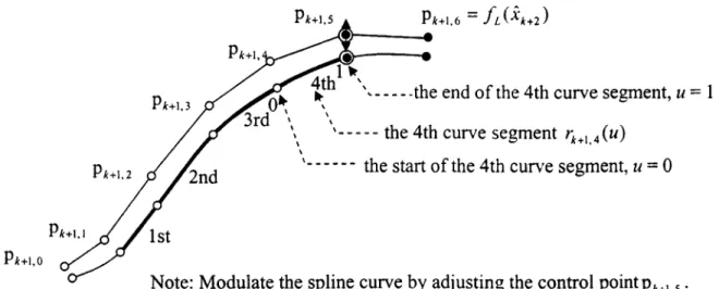
The design of the cam profile may not consider the dynamic capability of the control plant in ad-vance. Some dynamic limitations that degrade the slave motion generally apply; for example, a cut-ting machine tool may chatter due to over-large jerk, so the jerk has to be limited during the cut-ting process. Furthermore, maximal velocity and acceleration are limited by the motor and servo drive system. Consequently, the actual trajectory of slave motion may not be fulfilled, Eq.共14兲, but must be close to the ideal trajectory provided that it fits the specified constraints. Given its low sen-sitivity, the piecewise trajectory of the actual slave motion with respect to time is proposed to follow a cubic B-spline curve of fourth degree 关9兴, as shown in Fig. 5:

rk⫹1,j共u兲⫽F1,4共u兲pk⫹1,j⫺1⫹F2,4共u兲pk⫹1,j ⫹F3,4共u兲pk⫹1,j⫹1⫹F4,4共u兲pk⫹1,j⫹2,

共15兲

where r_k⫹1,j(u) represents the jth segment of the

(k⫹1)th time interval; j苸关1:4兴 denotes the

curve segment number andu⫽0 to 1 within each curve segment. p_k⫹1,j⫺1⬃p_k⫹1,j⫹2are the control points of the spline. F_1,4(u)⬃F4,4(u) are the

blending functions.

The fourth degree cubic B-spline, as shown in Fig. 8, exhibits second-order continuity. All the variables of the B-spline are defined below.

共i兲 p_k⫹1,0(⫽pk⫺4,5) denotes the initial control

point of the (k⫹1)th time interval, where p_k⫺4,5 is the previous position command of the slave at time (k⫺4)T and equivalently the fifth control point of the (k⫺4)th time interval.

共ii兲 p_k⫹1,1(⫽pk⫺3,5) denotes the first control

point of the (k⫹1)th time interval, where p_k⫺3,5 is the previous position of the slave at time (k

⫺3)T and equivalently the fifth control point of the (k⫺3)th time interval.

共iii兲 p_k⫹1,2(⫽pk⫺2,5) denotes the second

con-trol point of the (k⫹1)th time interval, where p_k⫺2,5is the previous position of the slave at time

(k⫺2)Tand equivalently the fifth control point of the (k⫺2)th time interval.

共iv兲 pk⫹1,3(⫽pk⫺1,5) denotes the third control

point of the (k⫹1)th time interval, where p_k⫺1,5 is the previous position of the slave at time (k

⫺1)T and equivalently the fifth control point of the (k⫺1)th time interval.

共v兲 p_k⫹1,4(⫽pk,5) denotes the fourth control

point of the (k⫹1)th time interval, where p_k,5is the previous position of the slave at time kT and equivalently the fifth control point of the kth time interval.

共vi兲 p_k⫹1,5denotes the position command of the slave motor yet to be determined, and is

equiva-Table 1

An example of cam profile table, both sets of data are scaled by their largest travel distance of one cam cycle. Master position x 0 0.1 0.2 0.3 0.4 0.5 0.6 0.7 0.8 0.9 1 Slave position f (x) 0 0.006 45 0.048 63 0.148 63 0.306 45 0.5 0.693 55 0.851 37 0.951 37 0.993 55 1

lently the fifth control point of the (k⫹1)th time interval.

共vii兲 p_k⫹1,6关⫽ f_L(xˆk⫹2)兴 denotes the sixth

con-trol point of the (k⫹1)th time interval, where f_L(xˆk⫹2) is derived from the cam profile position

at time(k⫹2)T, as indicated in Eq. 共14兲. Statements共i兲–共vii兲 include a total of seven un-knowns and six independent equalities. There is an extra degree of freedom left for the following op-timization problem: The slave’s position error be-tween the next unknown position commandpk⫹1,5

and the ideal cam profile position command f_L(xˆk⫹1) at time(k⫹1)T can be expressed as

e_k⫹1⫽p_k⫹1,5⫺ f_L共xˆ_k⫹1兲. 共16兲

The objective error function is defined in quadratic form as

E_k⫹1⫽储e_k⫹1储₂2⫽储p_k⫹1,5⫺ f共xˆ_k⫹1兲储₂2. 共17兲

To ensure that the velocity, acceleration, and jerk do not exceed the maximal values, (Vmax, Amax,

andJerkmax)allowed for the motor’s system, three

inequality constraints are imposed on the optimi-zation. The first, second, and third differentiation of the cubic B-spline curve at the start, u⫽0, of the fourth segment, can be expressed as follows:

r_ku_⫹1,4共0兲⫽⫺0.5pk⫹1,3⫹0.5pk⫹1,5, 共18a兲

r_kuu_⫹1,4共0兲⫽pk⫹1,3⫺2pk⫹1,4⫹pk⫹1,5, 共18b兲

r_kuuu_⫹1,4共0兲⫽⫺pk⫹1,3⫹3pk⫹1,4⫺3pk⫹1,5⫹pk⫹1,6. 共18c兲

Minimizing the objective error function subject to the constraints on velocity, acceleration, and jerk yields the one-dimensional constrained opti-mization problem:

Minimize 储p_k⫹1,5⫺ f共xˆ_k⫹1兲储₂2 共19a兲

subject to

再

兩r_ku_⫹1,4共0兲兩⭐Vmax 兩r_kuu_⫹1,4共0兲兩⭐A_max

兩r_kuuu_⫹1,4共0兲兩⭐Jerkmax.

共19b兲

共19c兲

共19d兲

The constrained optimization problem of a qua-dratic cost function has an easy to find optimal solution, p_k*_⫹1,5⫽ f_L(xˆk⫹1) with zero cost, when

none of the constraints is violated. According to Eqs. 共19a兲–共19d兲, the optimization problem may be reformulated as an unconstrained minimization problem as follows:

Minimize 储p_k⫹1,5⫺ f共xˆ_k⫹1兲储₂2⫹W_vg_v共p_k⫹1,5兲

⫹Waga共pk⫹1,5兲⫹WJgJ共pk⫹1,5兲, 共20兲

whereW_v, W_a, andW_J are the weighting factors of velocity constraint, acceleration constraint, and jerk constraint, respectively, and

g_v共p_k⫹1,5兲⫽

再

再

再

if 兩r_kuuu_⫹1,4共0兲兩⬍Jerkmax

0, if 兩r_kuuu_⫹1,4共0兲兩⭓Jerkmax.

共21c兲

In an extreme case that WvⰇWaⰇWJ, the

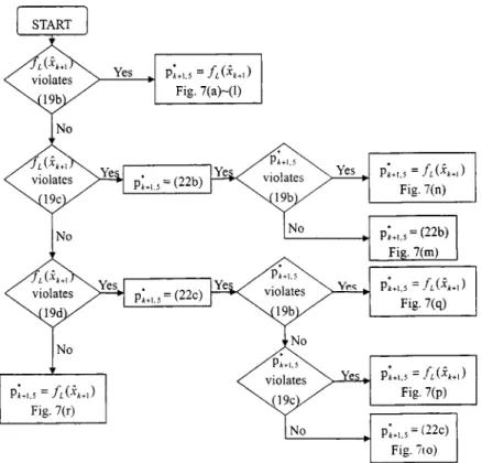
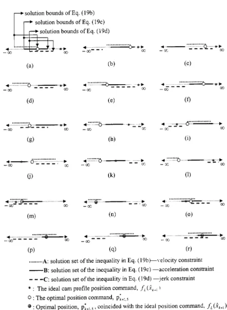
mini-mization problem implies a constraint violation priority that g_v is much more important than g_a and g_J. In practice, Eq. 共19兲 is highly nonlinear, existing techniques to find the global optimization are not guaranteed. One needs to enumerate all the possible cases for the global solution. Fig. 7 shows all the possible optimal solution for the extreme

case thatW_vⰇW_aⰇW_J.The bounds ofp_k⫹1,5for each of the constraints may be easily calculated from Eqs.共19b兲–共19d兲 by substituting the inequal-ity sign into equalinequal-ity sign, as follows:

p_k⫹1,5⫽2 sgn关r_ku_⫹1,4共0兲兴•V_max⫹p_k⫹1,3, 共22a兲 p_k⫹1,5⫽sgn关r_kuu_⫹1,4共0兲兴•A_max⫺p_k⫹1,3⫹2p_k⫹1,4, 共22b兲 p_k⫹1,5⫽⫺ 1 3sgn关rk⫹1,4 uuu _{共0兲兴Jerk} max⫺13pk⫹1,3 ⫹pk⫹1,4⫹13pk⫹1,6. 共22c兲

The optimal solution process may be depicted in the flow chart as shown in Fig. 6. According to the flow chart, the solution of the optimization prob-lem is unique, and thus guarantees to be the global optimum.

In Fig. 6, all possible cases are enumerated and categorized as follows. 共i兲 The ideal cam profile position command violates the velocity constraint, as shown in Figs. 7共a兲–7共l兲; 共ii兲 the ideal cam pro-file position command violates acceleration con-straint and does not violate velocity concon-straint, as

shown in Figs. 7共m兲 and 7共n兲; 共iii兲 the ideal cam profile position command violates only the jerk constraint, as shown in Figs. 7共o兲–7共q兲; 共iv兲 the ideal cam profile position command satisfies all of the constraints, as shown in Fig. 7共r兲.

5. Simulation and experimental results 5.1. Simulation of disturbance estimator

For simulation purposes, the nominal external disturbance is assumed to be a square wave func-tion:

共23兲

The amplitude a of the square wave is set to 4.8773 N m and the frequency of the square wave

is 1 Hz. Figs. 8共a兲 and 8共b兲 present the master’s

simulated angular velocity obtained using the pro-posed disturbance estimator feedback control and without using the disturbance estimator. The nominal parameters of the master motor defined in

Section 2 are Kˆ ⫽0.55 N m/A, Jˆ⫽0.093 kg m2_,

Fig. 8. 共a兲 Simulated angular velocity of the master. 共b兲 Simulated angular velocity of the master using disturbance estimator feedback control共zoom in兲.

Fig. 10. 共a兲 The tracking error of the master’s position for the zero-order interpolation method. 共b兲 The tracking error of the master for the third-order polynomial tracking method.共c兲 The tracking error of the master for the fourth-order polynomial tracking method.共d兲 The tracking error of the master for the fifth-order polynomial tracking method.

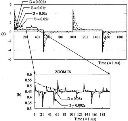
Figs. 9共a兲 and 9共b兲 show the maximum errors between the fed torque ␶L and the estimated

torque ␶ˆ_L for various time constants 共I兲. In Fig. 9共a兲, a smaller I yields a smaller mean torque er-ror. However, Fig. 9共b兲 reveals that a lower I yields a larger measurement noise. Furthermore, the measurement noise was assumed to be a zero-mean, normally 共Gaussian兲 distributed random signal in the simulation.

Both a larger mean torque error and a larger measurement noise reduce the tracking perfor-mance of the master, so the time constant must be neither too small nor too large. In the experiment, the time constant I of the disturbance estimator was set to ten times the current loop sampling time. As depicted in Fig. 8共b兲, the time constant I and the current loop sampling time are set to 0.01 s and 0.001 s, respectively.

5.2. Experimental results for tracking

performance of the electronic gearing process

Table 2 lists the parameter settings of the ECAM control. The accuracy of the tracking of the master’s velocity is characterized by the maxi-mum error between the actual position and the es-timated position. Figs. 10共a兲–共d兲 show that the maximum tracking error of the master’s position, using the fifth-order polynomial tracking control method, is zero when the master’s nominal mean speed is 10␲ rad/s. Table 3 shows the maximum tracking error of the master’s position for polyno-mial tracking control methods of various orders

(N⫽0 – 5).

5.3. Performance of the electronic cam process

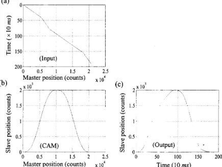
Fig. 11共b兲 shows an example of a reference tra-jectory that corresponds to the electronic cam mo-tion. According to a constant master speed of 10␲ rad/s and a maximum slave travel distance of 200␲ rad, the reference trajectory yields a 200␲ rad/s maximum slave speed, 1260␲ rad/s2 maxi-mum acceleration and 8120␲ rad/s3 maximum

Fig. 11. The piecewise tracking trajectory of the electronic cam motion:共a兲 the actual master’s position in real-time; 共b兲 the reference trajectory corresponding to the electronic cam motion;共c兲 the actual cam trajectory in real-time. Note that the unit ‘‘counts’’ means the encoder’s pulse counts and the resolution of the encoder is 2000 counts/revolution.

Table 3

The maximum tracking error of the master’s position for the Nth-order polynomial tracking control (N⫽0 – 5).

Order 0th 1st 2nd 3rd 4th 5th Max. err. 共counts/20␲ rad兲 11 17 3 1 1 0

Fig. 12. 共a兲 Cam profile error with the zero-order 共conventional兲 tracking method 共the maximum travel distance: 200 000 encoder’s counts兲. 共b兲 Cam profile error with the third-order polynomial tracking method 共the maximum travel distance: 200 000 encoder’s counts兲. 共c兲 Cam profile error with the fourth-order polynomial tracking method 共the maximum travel distance: 200 000 encoder’s counts兲. 共d兲 Cam profile error with the fifth-order polynomial tracking method 共the maximum travel distance: 200 000 encoder’s counts兲.

Table 4

An experimental example for the maximum tracking errors of the slave’s position in the encoder’s counts for the Nth-order polynomial master tracking control, the maximum travel distance is 200 000 encoder’s counts共equivalent to 200␲ rad兲.

Order 0th 1st 2nd 3rd 4th 5th Max. error 共encoder’s counts兲 395 655 83 17 2 1 rms error 194.9368 325.6317 45.2338 8.1915 0.9681 0.144 715 Cycle-to-cycle variation 0.590 083 0.449 440 0.140 121 0.075 427 0.129 316 0.072 357

Fig. 13. 共a兲 The tracking result of the slave velocity, acceleration, and jerk purely based on the Lagrange polynomial curve-fitting with no optimization.共b兲 The result of the slave velocity, acceleration, and jerk applying the optimization.

jerk. The master’s speed is generally not constant and may be harmonic, as shown in Fig. 7. The speed will exhibit the actual position of the master and the ideal cam trajectory, as shown in Figs. 11共a兲 and 11共c兲, respectively. This piecewise cam trajectory contains 191 points. Three performance indices are used to quantify the accuracy and con-sistency. The tracking accuracy of the slave

mo-and jerk, according to Lagrange polynomial curve-fitting with or without the aforementioned optimi-zation. Similarly, Table 5 indicates the tracking control performance, also for the Lagrange poly-nomial curve-fitting method with or without the aforementioned optimization.

5.4. Computational load on the CPU of the proposed ECAM tracking control

The selection of N depends on the accuracy de-manded. As stated above, tracking using a higher-order polynomial yields higher precision; how-ever, a tradeoff exists between the ‘‘order’’ of the polynomial used and the CPU time required. In

Fig. 14. Magnitudes of the sensitivities:共a兲 S K ¯ G_c , 共b兲 S J ¯ G_c , and共c兲 S B ¯ G_c

, in relation to the input frequency␻ at various time constantsI. Purely curve-fitting using Lagrange polynomial 1共scaled兲 共equivalent to 628.32 rad/s兲 20.12 共scaled兲 共equivalent to 12644 rad/s2兲 3980.95 共scaled兲 共equivalent to 2.50e06 rad/s3兲

practice, the computational time of the proposed algorithm共fifth-order tracking兲 is about 0.02 ms in a programming cycle on an Intel Pentium III 900-MHz CPU. The computational time of a program-ming cycle is much less than the PC-based sam-pling time, 10 ms.

6. Conclusion

The proposed disturbance estimator can effec-tively suppress the external disturbance and the high-frequency measurement noise, trading off de-lay time and the robustness of the estimator. As a result, higher-order polynomial fitting must be adapted for a cam profile with a farther travel dis-tance. The cam profile tracking is formulated as optimization in real-time control. A deterministic and unique solution is derived for all possible cases of tracking control. The proposed method is effective for general motion tracking control and guarantees a global optimal solution for practical control.

Acknowledgment

The authors would like to thank the National Science Council of the Republic of China for fi-nancially supporting this research under Contract No. NSC 91-2212-E009-050.

Appendix

The physical parameters of the motor may be dynamically varied, so the effect of parameter un-certainty must also be discussed. The well-known analysis of the modeling uncertainty is the ␮ analysis 关13兴. A more direct method is to analyze the sensitivities(S K ¯ Gc , S J ¯ Gc ,andS B ¯ Gc )of the transfer function G_c to the motor’s uncertain parameters, K¯ , J¯, andB¯ , respectively, where

G_c⫽ KK ¯_共Is⫹1兲 KJ¯ Is2_⫹共KB¯ I⫹K¯J兲_s⫹K¯B, 共A1兲 S K¯ Gc ⫽⳵Gc ⳵K¯ • K¯ Gc⫽ KJ¯ Is2_⫹KB¯Is KJ¯ Is2⫹共KB¯ I⫹K¯J兲s⫹K¯B, 共A2兲 S J ¯ Gc ⫽⳵Gc ⳵K¯ • K¯ Gc⫽ ⫺KJ¯Is2 KJ¯ Is2_⫹共KB¯ I⫹K¯J_兲s⫹K¯B, 共A3兲 S B ¯ Gc_⫽⳵Gc ⳵K¯ • K¯ G_c⫽ ⫺KB¯Is2 KJ¯ Is2_⫹共KB¯ I⫹K¯J_兲s⫹K¯B. 共A4兲

Figs. 14共a兲–14共c兲 show the magnitudes of the three sensitivities in relation to the input fre-quency, where the parameters of the master motor are all set as in Section 5. According to Eqs. 共A2兲 and 共A3兲, the magnitudes of the sensitivities, S

K¯ Gc andS J ¯ Gc

,are both small for low-frequency motion. Figs. 14共a兲 and 14共b兲 reveal that the magnitudes of the sensitivities, S K ¯ Gc and S J ¯ Gc

, are both less than 0.707 while the input frequency is lower than 1/I Hz. Furthermore, according to Fig. 14共c兲, the mag-nitude of the sensitivity S

B ¯ G_c

is less than 0.000 86 over the entire frequency domain. From Eqs. 共A1兲–共A3兲 and the foregoing discussion, the low time constant I of the disturbance estimator sup-presses the sensitivities,S

K ¯ G_c , S J ¯ G_c , and S B ¯ G_c . References

关1兴 Steven, Chingyei Chung, Tracking Control for the Electric Gear System. National Science Council of the Republic of China 845-012-011, 1995, pp. 1–35. 关2兴 Zhao, Qing-Feng, Advanced Design for Automatic

Control System. Chan Hwa Science and Technology Book Co., 2000, Chap. 4, pp. 1–26.

关3兴 Gavrilovic, A. and Heath, A. J., Prediction and Miti-gation of System Disturbances to Industrial Loads, Sources and Effects of Power System Disturbances. IEE Conference publication, 1982, pp. 227–230. 关4兴 Phillips, Charles L. and Nagle, H. Troy, Digital

Con-trol System Analysis and Design. Prentice-Hall Inter-national Editions, NJ, 1994, pp. 103–144.

关5兴 Yan, H. S., Tsai, M. C., and Hsu, M. H., An experi-mental study of the effects of cam speed on cam-follower systems. Mech. Mach. Theory 31, 397– 412 共1996兲.

关6兴 Yan, H. S., Tsai, M. C., and Hsu, M. H., A variable-speed method for improving motion characteristics of cam-following system. J. Mech. Des. 118, 250–258 共1996兲.

关7兴 Chen, Li-Shan, Follower Motion Design in a Variable-Speed Cam System. Master thesis, Institute of Me-chanical Engineering College of Engineering, National Chiao Tung University, 1995, pp. 1– 49.

关8兴 Dierchx, Paul, Curve and Surface Fitting with Splines. Oxford University Press, New York, 1993, pp. 75–91. 关9兴 Mortenson, Michael E., Geometric Modeling. John

M.S. degree in mechanical en-gineering at National Chiao-Tung University in 1995. He has been a Ph.D. candidate in mechanical engineering at Na-tional Chiao-Tung University since 2000. From 1995 to 2000, he served as a high school teacher of mathematics. His current research is in the motion simulator system for entertainment games.

Ph.D. in mechanical engineer-ing at Columbia University in 1989. He has been a full pro-fessor in mechanical engineer-ing at National Chiao-Tung University since 1996 and was appointed associated professor in 1989. His current research is in PC based control.