實質與貨幣內生成長模型的稅制改革政策 - 政大學術集成

全文

(1)國立政治大學經濟學系博士論文指導教授：張文雅博士. 政治大 Tax Reform Policies in Real and Monetary 立 ‧. ‧ 國. 學. Models of Endogenous Growth. n. er. io. sit. y. Nat. al. Ch. engchi. i n U. v. 研究生：李國豪撰中華民國九十九年七月.

(2) Abstract. The dissertation provides a theoretical framework to investigate the effects of tax policies, especially the tax reform, in real and monetary models of endogenous growth.. In. Chapter 2, by shedding light on the endogenous fertility choice, we set up a simple Romer (1986)-type endogenous growth model and show that, in a departure from the existing. 政治大. literature, a switch from a decrease in income tax rate to an increase in consumption tax rate. 立. so as to ensure a revenue-neutrality could be harmful, rather than favorable, to both growth. ‧ 國. 學. and welfare. In addition, we also conduct a simple numerical analysis to investigate the conditions in which the negative effect on growth and welfare occurs.. ‧. As to the monetary model, an endogenous growth model with endogenous labor-leisure. Nat. sit. n. al. er. Through the model, we found that the Mundell-Tobin effect and. io. established in Chapter 3.. y. choice and cash-in-advance (CIA) constraint which is only imposed on consumption is. i n U. v. the validity of consumption tax neutrality depend on the usages of tax revenue.. Ch. engchi. Next,. focusing on the distortions due to the production externality of capital and consumption tax, the optimal monetary policy is also derived.. Finally, we show that a switch from. consumption taxation to inflation taxation to finance a given stream of government expenditure, namely tax switch, enhances economic growth through the increase in labor supply in a CIA economy and the qualitative equivalence between MIU and CIA approaches is still valid.. i.

(3) Contents. Abstract ....................................................................................................................................... i Chapter 1. Introduction ........................................................................................................ 1 Reference ............................................................................................................. 9. Chapter 2. The Long-Run Growth and Welfare Effects of Tax Reform with. 政治大. Endogenous Fertility ....................................................................................... 13. 立. Introduction ........................................................................................................ 13. 2.2. The Model .......................................................................................................... 16. 2.3. Equilibrium Analysis .......................................................................................... 19. 2.4. The Steady-State Effects of Tax Reform ............................................................ 22. 2.5. Welfare Analysis ................................................................................................. 25. 2.6. Numerical Analysis ............................................................................................ 27. 2.7. Concluding Remarks .......................................................................................... 29. 2.8. Future Extensions ............................................................................................... 30. ‧. ‧ 國. 學. 2.1. n. er. io. sit. y. Nat. al. Ch. engchi. i n U. v. Appendix ........................................................................................................... 31 Figures and Tables ............................................................................................. 32 References ......................................................................................................... 35 Chapter 3. Consumption Tax, Seigniorage Tax, and Tax Switch Policy in a Cash-in-Advance Economy of Endogenous Growth .................................... 38. 3.1. Introduction ........................................................................................................ 38. 3.2. The Analytical Framework ................................................................................. 43. 3.2.1. Government ....................................................................................................... 43 ii.

(4) 3.2.2. Household-Producer .......................................................................................... 44. 3.2.3. Competitive Dynamic Equilibrium ................................................................... 46. 3.3. The Steady-State Effects of Tax Policies............................................................ 49. 3.4. The Optimal Monetary Policy ............................................................................ 53. 3.5. Tax Switch .......................................................................................................... 56. 3.6. Concluding Remarks and Future Extensions ..................................................... 59 Appendix A........................................................................................................ 61 Appendix B........................................................................................................ 64. 政治大. Figures ............................................................................................................... 66. 立. References ......................................................................................................... 68. ‧ 國. 學. Conclusions ....................................................................................................... 72 References ......................................................................................................... 74. ‧. io. sit. y. Nat. n. al. er. Chapter 4. Ch. engchi. iii. i n U. v.

(5) Chapter 1. Introduction. After the significant contribution of Solow (1956) and Swan (1956), neoclassical growth models have been extensively used in the research field of macroeconomics.. Due to the. features of the constant saving rate and diminishing marginal productivity of factors in a. 政治大. neoclassical production function, the per-capita output is bounded to converge to a stationary. 立. equilibrium in which the economic growth rate is tied to the exogenous demographic factors,. 學. Thus, the models can. not capture the reality of the sustained growth in per capita output.. Moreover, government. ‧. ‧ 國. such as the growth rate of population, and technologic progress rate.. policies can not affect the economic growth rate unless they can alter the demographic factors. y. Nat. io. sit. and technologic progress rate mentioned above.. n. al. er. To improve neoclassical growth model, Romer (1986) and Lucas (1988) start to develop. Ch. i n U. v. a so-called “endogenous growth theory” in which the assumption of the diminishing marginal. engchi. productivity of factors is discarded and the perpetual steady-state growth rate is an endogenous outcome of the economy.. Through the new framework, a platform is provided. for economists to analyze the relationship between macroeconomic policies and the economic growth rate. The common dimensions of macroeconomic policies are divided into two groups: the expenditure side and the revenue side.. In the expenditure side, the. effects of government expenditures with different features such as utility-enhancing or infrastructure are investigated under a given method of budget financing [such as Turnovsky (2000) and Zagler and Dürnecker (2003)].. 1. Comparatively, under a given form of.

(6) government expenditure, the effects of multiform financing approaches are evaluated in the revenue side [such as Turnovksy (1992) and Devereux and Love (1995)].. With both. frameworks, government can tune up the economy by altering the incentives of the optimizing agents. Among the plenty studies, one strand has emphasized on the effect of “revenue-neutral tax reform”.. In endogenous growth framework, the “revenue-neutral” tax reform implies. that an adjustment in the tax structure (for example, a switch from a decrease in the income tax rate to an increase in the consumption tax rate) finances a constant stream of government. 政治大. expenditure or lump-sum transfer, such as Pecorino (1993, 1994), Wen and Love (1998), and. 立. In this field, a general argument is that an income tax should be. 學. ‧ 國. Turnovsky (2000).1. replaced by a consumption tax, since a consumption tax will eliminate the bias against investment and savings inherent in the income tax system, thereby encouraging economic. ‧. growth and improving social welfare [Pecorino (1993, 1994), Wen and Love (1998), and. Nat. sit. y. Turnovsky (2000)]. Besides the theoretical researches, through the studies of the effects of. n. al. er. io. various types of taxes on the economic growth of developed countries within the OECD,. i n U. v. Johansson et al. (2008) suggest that if countries want to enhance their economic growth, they. Ch. engchi. would do well to move away from income taxes, especially corporate income taxes, toward less distortionary taxes such as consumption-based taxes. Under the consistent perspective, we find that there are still some insufficiencies in the discussions, such as the lack of an integration of family economics (for example, the endogenous fertility) which is emphasized by Becker (1988).2 1. 2. Referring to the empirical. In neoclassical growth model, the revenue-neutral tax reform implies that the adjustment in the tax structure maintains the tax revenue neutrality. Recent studies have highlighted the role of the endogenous fertility choice in terms of affecting macroeconomic performance. Barro and Becker (1989) analyze the optimal family size and growth in a model with altruism. Palivos and Yip (1993) and Yip and Zhang (1996) explore the interactions between output and the population growth rate and, accordingly, re-examine the Malthusian relationship in a Romer. 2.

(7) studies, such as Ermisch (1986), Sleebos (2003), and Grant et al. (2004), they have argued that taxation not only directly influences the macro goals, but also has the potential to affect fertility behavior.. Intuitively, in response to a tax reform, the fertility behavior of families. will change and in turn affect their time allocation between child rearing and working.. Thus,. the family’s fertility choice may alter the growth (and hence welfare) consequences of a tax reform. Inspired by the motives, in Chapter 2, we attempt to re-examine the effect of a revenue-neutral tax reform which involves a switch from a decrease in the income tax rate to. 政治大. an increase in the consumption tax rate so as to finance a constant stream of lump-sum. 立. transfer on the economic growth rate and social welfare in a simple Romer (1986)-type. ‧ 國. 學. endogenous growth model by incorporating the endogenous fertility choice. Focusing on the role of endogenous fertility rate, our findings are summarized as. ‧. follows.. First, we show that the revenue-neutral tax reform has an uncertain effect on the. Nat. n. al. The increase in the wage rate raises the. er. io. productivity of labor and hence the wage rate.. sit. y. equilibrium fertility rate. A decrease in the income tax rate increases the after-tax marginal. i n U. v. opportunity cost of child-rearing and thereby the fertility rate declines.. Ch. engchi. By contrast, an. increase in the consumption tax rate lowers the opportunity cost of fertility through the decline in the tax-adjusted shadow value of wealth.. Thus, tax reform has a mixed effect on. the equilibrium fertility rate. Second, the traditional notion argues that tax reform will directly raise the after-tax marginal productivity of capital and hence increase the balanced growth rate.. Our study indicates that in addition to this growth-enhancing effect, the. endogenous fertility rate will create an additional channel for tax reform to affect the steady-state growth rate.. In response to the shift away from an income tax towards a. consumption tax, if the steady-state fertility rate increases, the activities of child-rearing will (1986)-type endogenous growth model.. 3.

(8) reduce the time available to work and in turn lower the marginal productivity of capital.. As. a consequence, tax reform may decrease, rather than enhance, the balanced growth rate. Given the ambiguous effect on growth, a tax reform also has a mixed impact on social welfare.. The ambiguity of the growth and welfare effects obviously is in contrast to the. existing literature, for example, Pecorino (1993, 1994), Wen and Love (1998), and Turnovsky (2000).. However, our study cautions that in the presence of endogenous fertility, tax reform. could be harmful, rather than beneficial, to growth and welfare. In addition to the discussion in a real model of endogenous growth, we also evaluate the. In a monetary economy, the growth rate of 政治大. effects of tax policies in a monetary model.. 立. money supply provides another alternative for government to collect its revenue, i.e. the. ‧ 國. 學. seigniorage tax.. Based on the point, economists begin to concern about the relationship. between the growth rate of money supply and economic growth.. In the perspective on. ‧. capital accumulation, Mundell (1963) and Tobin (1965) conclude that higher monetary. Nat. sit. y. growth stimulates capital accumulation, i.e. the Mundell-Tobin effect. Moreover, Sidrauski. n. al. er. io. (1967) establishes an intertemporal optimizing model with money-in-utility-function (MIUF). i n U. v. and shows that the long-run capital stock is independent of the growth rate of monetary. Ch. e n gThereafter, chi. supply, i.e. the superneutrality of money.. Stockman (1981) introduces the. cash-in-advance (CIA) constraint developed by Clower (1967) and Lucas (1980) into neoclassical growth model and derives that the superneutrality of money is still valid when money balances are only required prior to carry out consumption, and the long-run capital stock decreases, when both consumption and investment are restricted by CIA constraint, i.e. the reversed Mundell-Tobin effect emerges. Afterward, along the development of endogenous growth theory, the Mundell-Tobin effect and the money superneutrality are broadly discussed and applied in the growth-rate sense in a variety of monetary growth models. By shedding light on the CIA constraint 4.

(9) which is only imposed on consumption, the superneutrality of money is a general result in the literature [Marquis and Reffett (1991), Mino (1997), and Chen and Guo (2008)]. Comparatively, some studies have argued that there exists mixed relationships between the growth rate of money supply and economic growth [Mino (1997), Dotsey and Sarte (2000), and Chang et al. (2000)].3. However, their frameworks have been embodied a common. feature, i.e. lump-sum transfer adjusts endogenously to maintain the balanced budget when government controls the growth rate of money supply. But, as shown in the empirical evidence, especially within the developing world, the government often balances its budget. 政治大. by adjusting its expenditure, thereby generating procyclical fiscal policies [Gavin and. 立. Roberto (1997) and Talvi and Végh (2005)]. Likewise, in Japan, Singapore, and Irish, not. ‧ 國. 學. only the lump-sum transfer, government can also adjust the government expenditure, such as the salary of public staff, to maintain the balanced budget recently.. Thus, by referring to the. ‧. literature which claims that the two methods of balanced-budget adjustment (the two usages. Nat. sit. y. of the tax revenue collected by a government) can cause different results in the economy. n. al. er. io. [Schmitt-Grohé and Uribe (1997), Pelloni and Waldmann (2000) and Guo and Harrison. i n U. v. (2004)], we are curious about how the different methods to maintain the balanced. Ch. engchi. government budget (the different usages of the tax revenue collected by a government) can alter the effects of tax policies. Furthermore, the mixed relationships between the growth rate of money supply and economic growth are also derived empirically. Some studies have found that there exists a negative relationship between the growth rate of money supply and economic growth [Gomme (1993), De Gregorio (1993), Barro (1995), and Gylfason and Herbertsson (2001)],. 3. Mino (1997) employs the two-sector model proposed by King et al. (1988) and concludes that the reversed Mundell-Tobin effect exists when labor supply is endogenous, but, money has no effect on the long-term growth rate if there is no labor-leisure choice of the households.. 5.

(10) others showed that the growth rate of money supply contributes a positive effect on economic growth [Bullard and Keating (1995)].. Thus, based on the present framework, we attempt to. provide a theoretical explanation of the mixed empirical findings. Besides the positive analysis, the optimal monetary policy also has been highly concerned among monetary economists for decades. In the pioneering study, Friedman (1969) argues that, to attain the social optimum, the monetary authority has to equate the private marginal cost of holding money (which is the nominal interest rate) to the social marginal cost of producing money (which is essentially nil).. 政治大. Thus, the nominal interest rate. should be zero to eliminate inefficiency when lump-sum tax is available, which is known as. 立. This proposition potentially implies that deflation is necessary for the. economy to attain the social optimum.. 學. ‧ 國. the Friedman rule.. Later, Phelps (1973) argues that a positive nominal. interest rate is necessary to achieve the efficiency if the revenue of government can only be. ‧. collected by distortionary taxes rather than lump-sum tax.. To reconcile the controversy, the. Nat. sit. y. presenting paper also aims to provide some suggestions for the optimality of Friedman rule.4. n. al. er. io. For another dimension, Cooley and Hansen (1992) employ a standard neoclassical. i n U. v. growth model with CIA framework of Lucas and Stokey (1983) and derive that, to replace. Ch. engchi. the tax on capital or labor income, the welfare-enhancing consequences of a seigniorage tax and a consumption tax are quite analogous in their quantitative assessment.. Moreover, in a. monetary framework, to enhance economic growth and improve social welfare, both consumption tax and seigniorage tax are regarded as a substitute for an income tax to finance a given stream of government expenditure or lump-sum transfer [Wen and Love (1998) and Palivos and Yip (1995)].. Although the two taxations have the similar property, but little. efforts have been made to focus on the comparison of the two alternatives.. 4. In the recent articles, Kocherlakota (2005) and Cunha (2008) have provided a comprehensive survey about the optimality of the Friedman rule.. 6.

(11) Recently, Ho et al. (2007) enable the labor-leisure choice in a monetary growth model with MIUF and derive that a switch from consumption taxation to inflation taxation to finance a given amount of government expenditure, namely tax switch, reduces leisure and accelerates the economic growth.. In addition, they briefly discuss the effect of tax switch in. a monetary growth model with the CIA constraint which is only imposed on consumption and find that the tax switch has no effect on resource allocation and welfare.. Nevertheless,. their discussion about the effects in CIA model is not clear and the results they derived are inconsistent with the qualitative equivalence between MIUF and CIA approaches.5. 政治大. Thus,. we are encouraged to extend the investigation and re-consider the qualitative equivalence of. 立. the tax switch in the two approaches.. ‧ 國. 學. To deal with the issues, in Chapter 3, we develop a monetary endogenous growth model with endogenous labor supply and CIA constraint which is only imposed on consumption.. ‧. Moreover, government is supposed to finance its lump-sum transfer or government Thus, besides the effects of the. sit. y. Nat. expenditure by consumption tax and seigniorage tax.. n. al. er. io. growth rate of money supply, the effects of consumption tax rate and tax switch can also be. i n U. v. investigated. Based on the framework, we find that: first, the different methods to maintain. Ch. engchi. the balanced government budget do result in a transformation in the effects of consumption tax rate and the growth rate of money supply respectively.. Intuitively, in addition to the. substitution effect due to the tax rate (the consumption tax rate and the growth rate of money supply), there exists an extra channel, namely the resource-withdrawing effect, to affect the resource allocation when tax policies is implemented with endogenous adjustment of government expenditure rather than lump-sum transfer.. Then the resource-withdrawing. effect can offset, even dominate, the substitution effect, and hence induce a change in the 5. In Wang and Yip (1992), they establish a qualitative equivalence between MIUF and CIA approaches, when CIA constraint is only imposed on consumption.. 7.

(12) consequence of tax policies.. Second, in the normative analysis, we found that the Friedman. rule which claim the zero nominal interest rate is no longer optimal if there exists the production externality of capital and consumption tax. Third, extending Ho et al. (2007), we find that even if the CIA constraint is only imposed on consumption, a switch from consumption taxation to inflation taxation to finance a given stream of government expenditure increases the steady-state growth rate through the decrease in leisure time.. This result not only contrasts with Ho et al. (2007) but also. proposes that the qualitative equivalence between MIUF and CIA approaches is still valid.. 政治大. Finally, the main consequences and some implications of each chapter are summarized. 立. in Chapter 4.. ‧. ‧ 國. 學. n. er. io. sit. y. Nat. al. Ch. engchi. 8. i n U. v.

(13) References Barro, R. J. and Becker, G. S., 1989, “Fertility Choice in a Model of Economic Growth,” Econometrica 57, 481-501. Barro, R. J., 1995, “Inflation and Economic Growth,” Bank of England Quarterly Bulletin, 166-176. Becker, G. S., 1988, “Family Economics and Macro Behavior,” American Economic Review 78, 1-13. Bullard, J. and Keating, J. W., 1995, “The Long-Run Relationship between Inflation and. 政治大. Output in Postwar Economies,” Journal of Monetary Economics 36, 477-496.. 立. Chang, W. Y., Hsieh, Y. N., and Lai, C. C., 2000, “Social Status, Inflation, and Endogenous. ‧. ‧ 國. 535-545.. 學. Growth in a Cash-in-Advance Economy” European Journal of Political Economy 16,. Chen, S. H. and Guo, J. T., 2008, “Velocity of money, equilibrium (in)determinacy and endogenous growth,” Journal of Macroeconomics 30, 1085-1096.. sit. y. Nat. io. er. Clower, R., 1967, “A Reconsideration of the Microfoundations of Monetary Theory,” Western Economic Journal 6, 1-9.. n. al. Cooley, T. F. and Hansen, G.. v i n C h1992, “Tax Distortions D., in engchi U. a Neoclassical Monetary. Economy,” Journal of Economic Theory 58, 290-316.. Cunha, A. B., 2008, “The Optimality of the Friedman Rule When Some Distorting Taxes are Exogenous,” Economic Theory 35, 267-291. De Gregorio, J., 1993, “Inflation, Taxation, and Long-Run Growth,” Journal of Monetary Economics 31, 271-298. Devereux, M. B. and Love, D. R. F., 1995, “The Dynamic Effects of Government Spending Policies in a Two-Sector Endogenous Growth Model,” Journal of Money, Credit, and Banking 27, 232-256.. Dotsey, M. and Sarte, P. D., 2000, “Inflation Uncertainty and Growth in a Cash-in-Advance. 9.

(14) Economy,” Journal of Monetary Economics 45, 631-655. Ermisch, J., 1986, “Impacts of Policy Actions on the Family and Household,” Journal of Pubic Policy 6, 297-318. Gavin, M. and Roberto P., 1997, “Fiscal Policy in Latin America,” NBER Macroeconomics Annual 12, MIT Press: Cambridge, Massachusetts, 11-61. Grant, J. et al., 2004, “Low Fertility and Population Ageing: Causes, Consequences, and Policy Options,” Santa Monica: RAND. Gomme, P., 1993, “Money and Growth Revisited: Measuring the Costs of Inflation in an. 政治大. Endogenous Growth Model,” Journal of Monetary Economics 32, 51-77.. 立. Guo, J. T. and Harrison, S. G., 2004, “Balanced-Budget Rules and Macroeconomic. ‧ 國. 學. (in)stability,” Journal of Economic Theory 119, 357-363.. Gylfason, T. and Herbertsson, T. T., 2001, “Does Inflation matter for Growth,” Japan and the. ‧. World Economy 13, 405-428.. Nat. sit. y. Ho, W. H., Zeng, J. and Zhang, J., 2007, “Inflation Taxation and Welfare with Externalities. io. n. al. er. and Leisure,” Journal of Money, Credit, and Banking 39, 105-131.. i n U. v. Johansson, Å., Heady, C., Arnold, J., Brys, B. and Vartia, L., 2008, “Tax and Economic. Ch. Growth,” OECD Working Papers 28.. engchi. King, R., Plosser, C. I., and Rebelo, S. T., 1988, “Production, Growth, and Business Cycle II: New Direction,” Journal of Monetary Economics 21, 309-342. Kocherlakota, N. R., 2005, “Optimal Monetary Policy: What We Know and What We Don’t Know,” Federal Reserve Bank of Minneapolis Quarterly Review 29, 10-19. Lucas, R. E. Jr., 1980, “Equilibrium in a Pure Currency Economy,” Economic Inquiry 18, 203-220. Lucas, R. E. Jr., 1988, “On the Mechanics of Economic Development,” Journal of Monetary Economics 22, 3-42.. 10.

(15) Lucas, R. E. Jr. and Stokey, N. L., 1983, “Optimal Fiscal and Monetary Policy in an Economy Without Capital,” Journal of Monetary Economics 12, 55-93. Marquis, M. H. and Reffett, K. L., 1991, “Real Interest Rates and Endogenous Growth in a Monetary Economy,” Economics Letters 37, 105-109. Mino, K., 1997, “Long-Run Effect of Monetary Expansion in a Two-Sector Model of Endogenous Growth,” Journal of Macroeconomics 19, 635-655. Mundell, R., 1963, “Inflation and Real Interest,” Journal of Political Economy 71, 280-283. Palivos, T. and Yip, C. K., 1993, “Optimal Population Size and Endogenous Growth,” Economics Letters 41, 107-110.. 立. 政治大. Palivos, T. and Yip, C. K., 1995, “Government Expenditure Financing in an Endogenous Growth. ‧ 國. 學. Model: A Comparison,” Journal of Money, Credit, and Banking 27, 1159-1178.. Pecorino, P, 1993, “Tax Structure and Growth in a Model with Human Capital,” Journal of. ‧. Public Economics 52, 251-271.. y. sit. io. al. er. 492-502.. Nat. Pecorino, P, 1994, “The Growth Rate Effects of Tax Reform,” Oxford Economic Papers 26,. v. n. Pelloni, A. and Waldmann, R., 2000, “Can Waste Improve Welfare?” Journal of Public Economics 77, 45-79.. Ch. engchi. i n U. Phelps, E., 1973, “Inflation in the Theory of Public Finance,” Swedish Journal of Economics 75, 37-54. Romer, P. M., 1986, “Increasing Returns and Long-Run Growth,” Journal of Political Economy 94, 1002-1037. Schmitt-Grohé, S. and Uribe, M., 1997, “Balanced-Budget Rules, Distortionary Taxes, and Aggregate Instability,” Journal of Political Economy 105, 976-1000. Sidrauski, M., 1967, “Rational Choice and Patterns of Growth in a Monetary Economy,” American Economic Review Papers and Proceedings 57, 534-544.. 11.

(16) Sleebos, J. E., 2003, “Low Fertility Rates in OECD countries: Facts and Policy Responses,” OECD Social, Employment, and Migration Working Papers 15. Solow, R. M., 1956, “A Contribution to the Theory of Economic Growth,” Quarterly Journal of Economics 70, 65-94 Stockman, A., 1981, “Anticipated Inflation and the Capital Stock in a Cash-in-Advance economy,” Journal of Monetary Economics 8, 387-393. Swan, T. W., 1956, “Economic Growth and Capital Accumulation,” Economic Record 32, 334-361.. 政治大 Developing Countries,” Journal of Development Economics 78, 156-190 立. Talvi, E. and Végh, C. A., 2005, “Tax Base Variability and Procyclical Fiscal Policy in. ‧ 國. 學. Tobin, J., 1965, “Money and Economic Growth,” Econometrica 33, 671-684. Turnovsky, S. J., 1992, “Alternative Forms of Government Expenditure Financing: A. ‧. Comparative Welfare Analysis,” Economica 59, 235-252.. Nat. sit. y. Turnovsky, S. J., 2000, “Fiscal Policy, Elastic Labor Supply, and Endogenous Growth,”. io. n. al. er. Journal of Monetary Economics 45, 185-210.. i n U. v. Wang, P. and Yip, C. K., 1992, “Alternative approaches to Money and Growth,” Journal of. Ch. engchi. Money, Credit, and Banking 24, 553-562.. Wen, J. and Love, D. R. F., 1998, “Evaluating Tax Reforms in a Monetary Economy,” Journal of Macroeconomics 20, 487-508. Yip, C. K. and Zhang, J., 1996, “Population Growth and Economic Growth: A Reconsideration,” Economics Letters 52, 319-324. Zagler, M. and Dürnecker, G., 2003, “Fiscal Policy and Economic Growth,” Journal of Economic Surveys 17, 397-418.. 12.

(17) Chapter 2. The Long-Run Growth and Welfare Effects of Tax Reform with Endogenous Fertility 2.1 Introduction The study of the effect of a revenue-neutral tax reform has been an important issue in In neoclassical growth 治政大 a switch from a decrease in the model, the so-called “revenue-neutral” tax reform involves 立 income tax rate to an increase in the consumption tax rate so as to ensure a balanced budget public finance and macroeconomics over the past three decades.. ‧ 國. 學. and hence tax revenue neutrality. Recently, intertemporal optimizing models have been. and social welfare.. ‧. extensively used to study the effects of tax reform on capital accumulation, economic growth, By developing various neoclassical growth frameworks, Summers. y. Nat. er. io. sit. (1981), Abel and Blanchard (1983), Auerbach et al. (1983), and Chamley (1985) find that the effects of tax reform depend on the model specifications, but in general can result in. n. al. Ch. i n U. v. efficiency gains, because a consumption tax involves less distortion than income tax.. engchi. Specifically, a consumption tax will eliminate the bias against investment and savings inherent in the income tax system, thereby encouraging capital accumulation and improving future life standards.. This beneficial effect is still valid in the endogenous growth models.1. In a one-sector AK model with endogenous leisure-labor discretion, Turnovsky (2000a) finds that replacing the income tax rate with a consumption tax has a positive effect on economic growth and welfare.. 1. Pecorino (1993, 1994) employs a two-sector Lucas (1988) model and. In endogenous growth framework, the “revenue-neutral” tax reform implies that a switch from a decrease in the income tax rate to an increase in the consumption tax rate to finance a constant stream of government spending or lump-sum transfer.. 13.

(18) also refers to a positive effect of tax reform on growth and welfare. Wen and Love (1998) further show that the favorable growth and welfare effects can apply to a monetary model. By shedding light on the endogenous fertility choice, this paper attempts to re-examine the effects of a revenue-neutral tax reform on growth and welfare in a simple Romer (1986)-type endogenous growth model. Empirical studies, such as Ermisch (1986), Sleebos (2003), and Grant et al. (2004) have argued that taxation not only directly influences the macro goals, but also has the potential to affect fertility behavior.. Intuitively, in response to. a tax reform, the fertility behavior of families will change and this in turn will affect their. 政治 Thus, 大 the family’s fertility choice will. time allocation between child rearing and working.. 立. alter the growth (and hence welfare) consequences of a tax reform.. We are convinced that. ‧ 國. 學. the growth and welfare effects of a tax reform turn out to be rather different from the common predictions in a model with an exogenously-determined fertility rate.. ‧. Whatever the relevance of these analyzes to tax reform, they remain silent in exploring. Nat. sit. n. al. er. Batina (1987) and Kobayashi (1996) are among the exceptions. Batina (1987). io. reform.2. y. the implications of an endogenous fertility rate for the growth and welfare effects of a tax. i n U. v. examines the validity of consumption tax neutrality in an overlapping-generations model. Ch. engchi. taking into consideration the endogenous fertility choice. By extending Batina’s (1987) framework, Kobayashi (1996) investigates the effects of tax reform on capital accumulation and social welfare in the presence of an endogenous fertility choice.. However, both Batina. (1987) and Kobayashi (1996) conduct their analysis in a neoclassical growth (an exogenous growth) framework. Little is known, however, about the impact of tax reform on economic growth and social welfare in an endogenous growth setting under considerations of endogenous fertility choice.. 2. Please refer to footnote 2 in Chapter 1.. 14.

(19) The main findings of this paper are summarized as follows. First of all, we show that a switch from an income tax to a consumption tax has an uncertain effect on the equilibrium fertility rate. A decrease in the income tax increases the after-tax marginal productivity of labor and hence the wage rate.. The increase in the wage raises the opportunity cost of. child-rearing and, as a result, the fertility rate declines. By contrast, an increase in the consumption tax lowers the opportunity cost of fertility through the decline in the tax-adjusted shadow value of wealth.. Thus, tax reform has a mixed effect on the. equilibrium fertility rate. Second, the traditional notion argues that tax reform will directly. 政治大. raise the after-tax marginal productivity of capital and hence increase the balanced growth. 立. Our study indicates that in addition to this growth-enhancing effect, the endogenous. 學. ‧ 國. rate.. fertility rate will create an additional channel for tax reform to affect the steady-state growth rate. In response to the tax shift away from an income tax towards a consumption tax, if the. ‧. steady-state fertility rate increases, the activities of child-rearing will reduce the time. Nat. Thus, tax reform. sit. y. available to work and in turn lower the marginal productivity of capital.. n. al. er. io. may decrease, rather than enhance, the balanced growth rate. Given the ambiguous effect. i n U. v. on growth, a tax reform also has a mixed impact on social welfare.. Ch. engchi. The ambiguity of the. growth and welfare effects obviously are in contrast to the existing literature, for example, Summers (1981), Auerbach et al. (1983), Chamley (1985), Pecorino (1993, 1994), Wen and Love (1998), and Turnovsky (2000a). However, our study cautions that in the presence of endogenous fertility tax reform could be harmful, rather than beneficial, to growth and welfare. The remainder of the paper is organized as follows.. In Section 2 we first construct the. optimizing behavior of the representative agent with endogenous fertility choice. Section 3 outlines the dynamic properties and the steady-state relationships of the economy.. Sections. 4 and 5 in turn examine the effects of tax reform on the fertility rate, the balanced growth rate, 15.

(20) and social welfare. our conclusions.. Section 6 conducts a simple numerical analysis.. Section 7 summaries. Finally, Section 8 provides some future extensions.. 2.2 The Model Consider an economy consisting of a continuum of infinitely-lived identical agents and a government.. A representative agent seeks to maximize the discounted sum of future. instantaneous utilities:3 . Wt   [ln ct  0. nt1  1   t ] e dt , 1 . (1). 政治大. where ct is per capita consumption, nt is the fertility rate or the population growth rate,. 立.   (0, ) is a non-negative parameter representing the elasticity of the marginal utility of. ‧ 國. 學. fertility, and  is a constant rate of time preference ( 0    1 ).4. The specification of. ‧. equation (1) is in accordance with the standard practice of the literature on endogenous fertility, for example, Razin and Ben-zion (1975), Eckstein and Wolpin (1985), Eckstein et al.. y. Nat. Sala-i-Martin (2004), Yip and Zhang (1996,1997).. n. al. Ch. These studies all emphasize that each. er. io. sit. (1988), Palivos and Yip (1993), Wang et al. (1994), Palivos (1995), and Barro and. i n U. v. agent’s utility depends not only on consumption, but also on the fertility rate.. engchi. The fertility. rate enters the utility function originating from the fact that each agent cares about the number of children. At each instant of time, the representative agent is bound by two kinds of constraints. First, the budget constraint links the accumulation of physical capital to any difference between its income (the sum of output and government transfers) and its expenditure (the 3. Since the labor-leisure choice does not alter the favorable growth and welfare effects of tax reform, to emphasize the role of fertility, we abstract it.. 4. By following Wang et al. (1994), Palivos (1995), and Yip and Zhang (1996, 1997), we assume that there is no immigration and that the mortality rate is zero. This implies that there is a one-to-one correspondence between the population growth rate and the fertility rate.. 16.

(21) sum of consumption, tax payments, and the expense of maintaining the existing population). Accordingly, the agent’s flow budget constraint is given by: kt  (1   I ) Akt  (lt  kt )1  Rt  nt k t  (1   ct )ct ,. (2). where an overdot denotes the time derivative, kt is the private capital stock, lt is labor time, kt is the average economy-wide level of capital stock,   (0,1) , Rt presents real. lump-sum transfers from the government,  I is the income tax rate, and  ct is the consumption tax rate. The production function in equation (2) is the Romer (1986)-type. 政治大 leads to a parallel increase in its stock of knowledge. This specification allows us to 立 specification of the knowledge spillover effect whereby an increase in a firm’s capital stock. ‧ 國. 學. generate sustained growth in the model.. Second, we assume that the time endowment is normalized to unity and that the. ‧. representative agent allocates the time endowment to labor time and child-rearing. Thus,. y. (3). io. er. 1  lt   (nt ) ,. sit. Nat. the time allocation constraint is:. where  (nt ) is the time cost of child-rearing. Without loss of generality, we further follow. al. n. v i n Yip and Zhang (1997) to assume aC constant cost of child rearing, i.e., h e nunit gchi U.  (nt )  nt  .5. The intertemporal optimizing problem for the agent is to maximize equation (1) subject to equations (2) and (3). Substituting equation (3) into (2) and letting t be the co-state variable of the current-value Hamiltonian associated with equation (2), the optimum conditions necessary for this maximization are: 1  t 1   ct  , ct 1 nt 5. .  t [1   I 1   Akt  1  nt   kt1  kt ] ,. See Yip and Zhang (1997, pp.100-101) for details on this linear cost function.. 17. (4a) (4b).

(22) t  t [   nt  1   I Akt  1 1  nt  1 kt1 ] ,. (4c). kt  (1   I ) Akt  1  nt  1 kt 1  Rt  nt kt  (1   ct )ct ,. (4d). lim t kt e   t  0 .. (4e). t . Equation (4a) implies the equality between the marginal utility of consumption and the tax-adjusted shadow value of wealth. Equation (4b) indicates that the marginal benefit of fertility equals the opportunity cost of fertility.. The marginal benefit of fertility is the. marginal utility of fertility, while the opportunity cost of fertility includes the after-tax. 政治大. marginal productivity of labor plus the per capita capital stock, adjusted for the shadow value. 立. of wealth. Equation (4c) is the Euler condition governing the optimal choice between. ‧ 國. 學. consumption and capital accumulation (which is crucially related to the rate of return on consumption and the after-tax rate of return on capital). Finally, equation (4d) is the flow. ‧. budget constraint and equation (4e) is the transversality condition for the capital stock.. Nat. sit. y. In line with Pecorino (1993, 1994) and Wen and Love (1998), we assume that the. n. al. er. io. government collects income and consumption taxes and rebates these tax revenues in a. i n U. v. lump-sum transfer, Rt , to households. Thus, the government budget constraint is given by:. Ch. i. e.  c h  I Akt (1  nt  )1n k t1g   ct ct  Rt .. . (5). Since we do not investigate the effects of government expenditure, we abstract government expenditure from our model.. Besides, in order to ensure sustained steady-state growth, we. assume further that the government’s transfer payment is set as a fraction,  , of output: Rt  Akt  1  nt  1 k t1 ,. 0    1.. (6). The revenue-neutral tax reform involves a tax shift away from an income tax towards a consumption tax, financing the constant stream of lump-sum transfer.. In line with this, we. set the ratio  as given, and the income tax rate  I as a policy parameter.. 18. As a.

(23) consequence, the consumption tax rate becomes endogenous to ensure the balanced budget of the government.. 2.3 Equilibrium Analysis. Since agents are assumed to be identical in a representative agent framework, in a symmetric equilibrium all agents own the same amount of capital, i.e., kt  kt . Under the symmetric equilibrium, equations (4b)-(4d) and (5) with (6) can be rewritten as follows: 1 nt. .  t [1   I 1   A1  nt   kt  k t ] ,. (4b)'. t t. (4c)'. 政治大 立   n  (1   )A(1  n  ) , 1. t. I. t. (   I ) A(1  nt  )1 kt   ct ct .. ‧. ‧ 國. 學. kt  (1   I ) A1  nt  1 kt  Rt  nt kt  (1   ct )ct ,. (4d)' (7). sit. y. Nat. It follows from equation (7) that to guarantee a positive rate of consumption tax (  ct  0 ), we. io. er. assume    I  0 throughout the paper.. By following Barro and Sala-i-Martin (2004), we define xt  ct kt as a transformed. al. n. v i n variable since the growth rates ofCch t and k t will be U e n g c h i the same along the balanced growth path.. Accordingly, equations (4a), (4b)' and (7) allow us to derive the following. instantaneous relationship for the endogenous fertility rate: nt  n( xt , I ) , where n x . 1. .  0 , n I . (8). A(1  nt  )  [nt  (1   )  (1  nt  )]  0 , and   nt  1[(1   I )   1. (1   )A(1  nt )   1]  nt  (1   I ) (1   ) 2 A(1  nt )  1  (   I )(1   )A(1  nt )   0 . In addition, putting equations (4d)', (6) with kt  kt , and (7) together, the aggregate resource constraint (i.e., the goods market equilibrium) is given by:. 19.

(24) kt  A(1  nt  )1 kt  ct  nt k t .. (9). From equations (4a) and (4c)', the modified Keynes-Ramsey rule is as follows: . ct      nt  (1   I )A(1  nt )1  ct ct , ct 1   ct  ct. (10). Given xt  ct kt , equations (9) and (10) immediately yield: xt ct kt  ct .    xt  [1   (1   I )] A(1  nt  )1    ct xt ct kt 1   ct  ct. (11). By using the government budget constraint in equation (7) and the instantaneous relationship of fertility in equation (8), it is easy to simplify the above equation as:. 政治大. xt   {xt  [1   (1   I )] A(1  nt  )1   } , xt. 立. (1   ct ).  0 .6. . (1  nt  ). By substituting equation (8) into (12), we. 學. [1   ct (1   ). ‧ 國. where  . (12). xt n x ]. model.. ‧. can constitute the dynamic system by a differential equation in terms of xt in our growth. y. Nat. io. sit. Proposition 1. (The Existence, Uniqueness, and Stability of the Steady-State Growth. n. al. er. Equilibrium) In the presence of the endogenous fertility rate, under a revenue-neutral tax 6. Ch. i n U. v. Since the transfer payment ratio  is exogenously given and the income tax rate  I is a policy parameter,. engchi. from equations (7) and (8), we can derive  ct  (   I ) A[1  n( xt , I ) ]1 / xt . equation with respect to time further yields:. Differentiating this. ct n  xt x  [1  (1   ) t n x ]  t . This implies that under  ct 1  n t  nt xt. the tax reform  ct may be time-varying, changing over time and adjusting with the consumption-capital ratio side by side, even though the income tax rate changes once and for all (rather than changing over time). Substituting this relationship into equation (11) then gives: x t   {xt  [1   (1   I )] A(1  nt  )1   } . xt. It is easy to further derive equations (7) and (8) so that. . (1   ct ) [ xt  (   I ) A(1  nt  )1 ]   0.  1  2 1 (1   ) ] [1   ct xt n x ] xt nt [ (1   I )(1   )A(1  nt  )    nt (1   I ) (1   ) A(1  nt  ) (1  nt  ). 20.

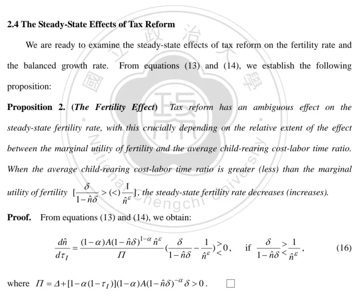
(25) reform there exists a unique steady-state growth equilibrium which is locally determinate. Proof.. At the steady-state growth equilibrium, the economy is characterized by xt  0 , and. xt and nt are at their steady-state values, namely, xˆ and nˆ . Hence, from equation (12) with xt  0 and equation (8), we have: xˆ  [1   (1   I )] A(1  nˆ  )1   ,. (13). xˆ  nˆ  [(1   I )(1   )A(1  nˆ )   1]  (   I ) A(1  nˆ  )1 .. (14). The xt  0 locus traces all combinations of ( xt , nt ) which satisfy (13) and the NN locus. 政治大 NN is upward sloping in the. traces all combinations of ( xt , nt ) which satisfy (14). As shown in Figure 1, locus xt  0. 立. is downward sloping, while locus. ( xt , nt ) space, i.e.:. ‧ 國. 學. dxt dxt | x t  0  [1   (1   I )](1   )A(1  nˆ  )   0 and | NN    0 . dnt dnt It is evident from Figure 1 that the xt  0 locus intersects the xt -coordinate at. y. . ), along the xt  0 locus xt has a lower bound, xt min   . On the other. sit. 1. Under the restriction of non-negative working. Nat. hours ( nt . ‧. [1   (1   I )] A    0 when nt  0 .. er. io. hand, Figure 1 indicates that the NN locus intersects the xt -coordinate at  (   I ) A  0. al. n. v i n xt   , theCfertility rate will converge to hengchi U. when nt  0 . For. nt . 1. .  0.. As is evident. from Figure 1, the steady-state growth equilibrium exists and is unique.7 By substituting equation (8) into (12) and expanding the resulting equation in the neighborhood of the steady state, we thus obtain the characteristic root of the dynamic system.  as follows:   xˆ {1  [1   (1   I )](1   ) A(1  nˆ )  n x }  0 .. (15). This implies that there is an upward-sloping xt locus in the ( xt , xt ) space in the phase 7. In effect, the x t  0 locus is concave in nt and the NN locus could be convex or concave in nt . Nevertheless, these cases do not affect the existence and uniqueness of our steady-state growth equilibrium.. 21.

(26) diagram of this dynamic system, as shown in Figure 2.. As documented by the literature on. dynamic rational expectations models, for example, Buiter (1984) and Turnovsky (2000b), if the number of unstable roots equals the number of jump variables, then there exists a unique perfect-foresight equilibrium solution.. Since xt is a jumping variable and the dynamic. system has one root with a positive real part, as indicated in equation (15), the economy has a □. unique steady-state growth equilibrium which is locally determinate.. 2.4 The Steady-State Effects of Tax Reform. 政治大. We are ready to examine the steady-state effects of tax reform on the fertility rate and the balanced growth rate.. Proposition 2. (The Fertility Effect). Tax reform has an ambiguous effect on the. ‧. ‧ 國. 學. proposition:. 立From equations (13) and (14), we establish the following. steady-state fertility rate, with this crucially depending on the relative extent of the effect. y. Nat. io. sit. between the marginal utility of fertility and the average child-rearing cost-labor time ratio.. utility of fertility [ 1  nˆ  Proof.. a l1. v i n  ( )  C ] , the steady-state fertility rate decreases (increases). hengchi U nˆ n. . er. When the average child-rearing cost-labor time ratio is greater (less) than the marginal. From equations (13) and (14), we obtain: (1   ) A(1  nˆ )1 nˆ  dnˆ  1   )0, (  d I  1  nˆ nˆ . where     [1   (1   I )](1   ) A(1  nˆ  )    0 .. if. .  1 ,  1  nˆ  nˆ . (16). □. A simple but intuitive explanation to the result of Proposition 2 is as follows. The tax reform involves a switch from a decrease in the income tax rate to an increase in the consumption tax rate so as to ensure a balanced budget. In response to a decrease in the income tax, the after-tax marginal productivity of labor increases and, accordingly, the wage 22.

(27) rate rises. The increase in the wage will raise the opportunity cost of child-rearing and, as a result, the equilibrium fertility rate will decline. On the other hand, under a revenue-neutral tax reform the decrease in the income tax should be associated with an increase in the consumption tax.. In contrast to the fertility effect of income tax, increasing the. consumption tax rate lowers the opportunity cost of fertility through the decline in the tax-adjusted shadow value of wealth, as shown in equation (4a). Thus, tax reform may result in an increase in the fertility rate.. To sum up, if the former effect is larger (smaller). than the latter one, the average child-rearing cost-labor time ratio will be greater (less) than the marginal utility of fertility. effect on the fertility rate.8. 政治大. As a result, tax reform will give rise to a harmful (favorable). 立. ‧ 國. 學. We now turn to a discussion of the growth effect of tax reform. Proposition 3. (The Growth Effect). Tax reform involving a shift away from an income tax. ‧. towards a consumption tax can lead to a deterioration, rather than an improvement, in the. Nat. sit. al. n. rate ˆ is given by:. er. It follows from equation (10) with ct  0 that the economy’s balanced growth. io. Proof.. y. balanced growth rate.. Ch. engchi. i n U. v. ˆ  (1   I )A(1  nˆ  )1    nˆ .. (17). Differentiating equation (17) with respect to  I , we then have: dˆ dnˆ    A(1  nˆ  )1  [1  (1   I ) (1   ) A(1  nˆ  )   ] 0. d I d I . (18). Equation (18) states that the effect of tax reform on the balanced growth rate is ambiguous,. 8. In fact, the secondary effect stemming from the change in the consumption-capital ratio will jointly affect the steady-state fertility rate. However, for ease of understanding, we roughly explain the intuition of the tax reform effect on the fertility rate by highlighting the direct effect of tax reform.. 23.

(28) □. being related to the steady-state fertility effect of tax reform.. The result reported in Proposition 3 sharply contradicts the common notion in the tax reform literature, as in Summers (1981), Auerbach et al. (1983), Chamley (1985), Pecorino (1993, 1994), Wen and Love (1998), and Turnovsky (2000a).. In addition to the. growth-improving effect by virtue of the increase in economic growth, the endogenous fertility creates an additional channel for tax reform to affect the steady-state growth rate. To be more specific, in our model tax reform affects the balanced growth rate through two channels when the endogenous fertility is considered. As shown in equation (18), the. 政治大. first channel (which recovers the traditional effect in the tax reform literature) is that tax. 立. balanced growth rate, i.e.,. dˆ 0. d I. 學. ‧ 國. reform directly raises the after-tax marginal productivity of capital and hence increases the The second channel captures the induced effect. ‧. stemming from the endogenous response of the steady-state fertility rate to tax reform,. Nat. sit. y. which alters the time allocation of household and the per capita capital stock distributed to. n. al. er. io. the newborn. In response to the tax shift away from an income tax towards a consumption tax, if the steady-state fertility rate falls (. Ch. v. dnˆ  0 ), the additional channel will reinforce the d I. engchi. i n U. growth-improving effect of tax reform. However, if the steady-state fertility rate rises (. dnˆ  0 ), the activities of child-rearing will reduce the time it has available for work and d I. more capital stock will be distributed to the newborn. Thus, the additional channel will be harmful to economic growth. Once the negative effect is substantially large, the balanced growth rate will decrease (i.e.,. dˆ  0 ), rather than increase, followed by tax reform. d I. 24.

(29) 2.5 Welfare Analysis. This section examines the effect of tax reform on welfare. Since our framework is the. AK model of endogenous growth and there is no transitional dynamics in response to an unanticipated permanent tax reform (referring to Figure 2), we deal with the lifetime utility attained on the balanced growth path along the lines of Yip and Zhang (1997). Along the steady-state growth equilibrium with a given initial private capital stock k0 , private consumption and capital grow at a common rate ˆ (which is a function of  I ). The time paths of private consumption and the capital stock are therefore given by:. 政治大立c  c e , and k  k e , ˆ t. t. ˆ t. t. 0. ‧ 國. With equation (19), we immediately have. 學. where c0 is endogenously determined.. (19). 0. c0  k 0 xˆ by using x  c k . As there is no transitional dynamics, the impact of tax reform. ‧. on c0 is equivalent to the steady-state effect of tax reform on xˆ . Moreover, the fertility Based on the. sit. y. Nat. rate is at its steady-state value nˆ (which is also a function of  I ).. io. al. n. function as follows:. er. above-mentioned information, equation (1) allows us to derive the equilibrium lifetime utility. Ch. 1 Wˆ  [ln xˆ  ln k 0 . . ˆ. 1 . nˆ. i U 1 n .. e n gc h1i . ]. v. (20). According to equation (20), we have: Proposition 4. (The Welfare Effect). In the presence of the endogenous fertility rate, tax. reform can decrease social welfare. Proof.. Differentiating equation (20) with respect to  I and manipulating the resulting. equation with the steady state effect derived above and the relation nˆ  from equation (14), we derive:. 25.

(30) dWˆ 1 1 1 dnˆ  0,  (  )A(1  nˆ  )1  d I  xˆ  d I . where   . 1. . {[. 1. . . (1   I ). (21). 1 1 ˆ  )  { [1   (1   I )]  (1   I )   A  n ] ( 1  )  ( 1 xˆ  xˆ  (   I ) A(1  nˆ  )1 1. xˆ  (   I ) A(1  nˆ )1. }} ..  0.. The Appendix provides a detailed deduction of the sign of □. Similar to the growth effect, except for the direct welfare-improving effect of tax reform, the endogenous fertility choice creates an induced effect for tax reform to affect social. 政治大 tax reform, which is independent of the steady-state fertility rate. 立. welfare. Equation (21) clearly indicates that the first term on the RHS is the direct effect of It reflects the components. ‧ 國. welfare.9. 學. of the efficiency gains and growth-improvement of tax reform, thereby improving social The second term on the RHS is the induced effect of tax reform stemming from a. ‧. change in the fertility rate. As shown in Proposition 2, the effect of tax reform on the. sit. y. Nat. steady-state fertility rate is ambiguous and hence the induced effect of tax reform on social. io. n. al. er. welfare is also ambiguous. If the fertility effect of tax reform is positive (. i n U. dnˆ  0 ) and is d I. v. substantial, the induced effect will dominate the direct effect and, consequently, tax reform. Ch. engchi. will be harmful, rather than beneficial, to social welfare. It is important to emphasize that while the previous studies in general refer to a favorable welfare effect, our results predict a mixed impact on social welfare. Therefore, it worth conducting a simple numerical analysis to further investigate under what conditions the harmful growth and welfare effects occur to which we now turn.. 9. The balanced growth condition (13) implies that (1 xˆ  1  )  0 .. 26. xˆ  . holds.. As a consequence, we have.

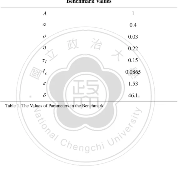
(31) 2.6 Numerical Analysis. In Sections 4 and 5, we have argued that tax reform can retard growth and decrease welfare. Meanwhile, we have also pointed out that the endogenous fertility rate is central in terms of governing the relationship between tax reform and growth (welfare). One may be interested in which parameters are the deterministic factors, how the results change with these parameter values, and whether or not the negative effect of tax reform on growth (welfare) can exist in practice. In this section we will conduct a simple numerical analysis to answer these questions.. 政治大. We first calibrate the values of parameters in our model. These benchmark values are. 立. summarized in Table 1. By following Pecorino (1994), we set the time preference rate as. ‧ 國. 學.   0.03 , the government transfer payment ratio as   0.22 , and the capital share as   0.4 (which is in the range specified in the common macro literature). For simplicity,. ‧. the technology parameter is specified as A  1 . In line with Chatterjee and Turnovsky. y. In addition, in the benchmark the growth. sit. Nat. (2007), the income tax rate is set as  I  0.15 .. n. al. er. io. rate is assumed to be   0.018 which accords with the average growth rate for the US from. i n U. v. 1890-1990, as reported in Barro and Sala-i-Martin (2004). According to the social statistic. Ch. engchi. data of OECD, the average fertility rate in America during 1997-2006 was about 0.0202. Thus, from equation (17), the time cost of child-rearing can be calibrated as   46.1 . Given that, equation (13) allows us to calculate the consumption-capital ratio as xˆ  0.1624 that satisfies the US data. Since the US consumption-output ratio is about 0.73 (see, for example, Christiano, 1988) and the capital-output ratio is in the range of 2.4 (Lucas, 1990) to 10.59 (Christiano, 1988), the reasonable consumption-capital ratio is allocated within the range of 0.07 to 0.3. Finally, from equations (7) and (14), we can calibrate   1.53 and. ˆc  0.0865 . The consumption tax rate we calibrate here is located within this reasonable range, namely, 5%~25%, for OECD countries in 2009. 27.

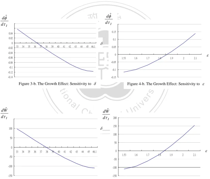
(32) . 1 holds true, tax 1  nˆ nˆ  dnˆ reform will give rise to an increasing effect on the fertility rate, i.e.,  0 and this may d I Propositions 2-4 clearly indicate that if the condition. generate a negative effect of tax reform on both growth (. . dWˆ dˆ  0 ) and welfare (  0 ). d I d I. Based on the benchmark parameters above, Figure 3-a shows that if the cost of child-rearing is substantially low, namely,   43.95 in our simulation, tax reform will increase the fertility rate. The revenue-neutral tax reform involves a reduction in income taxation with a. 政治大 the after-tax marginal productivity of labor and hence the wage rate, since a higher wage rate 立. move to consumption taxation. As noted in Proposition 2, a lower income tax rate increases. ‧ 國. effect on the equilibrium fertility rate.. 學. raises the opportunity cost of child-rearing and, as a result, tax reform gives rise to a negative However, the magnitude of the fertility effect is. ‧. lessened as the time cost of child-rearing,  , is relatively small.. A small value of . sit. y. Nat. implies that child-rearing is less time-consuming, which increases the available time for. io. rate.. er. households to work. The increase in the labor supply will decrease the equilibrium wage. al. Thus, the income tax effect on the fertility rate is offset. As a result, the consumption. n. v i n C hthe income tax effect, tax effect is more likely to dominate e n g c h i U resulting in an increase in the fertility rate.. Most previous studies, such as Summers (1981), Auerbach et al. (1983), Chamley (1985), Pecorino (1993, 1994), Wen and Love (1998), and Turnovsky (2000a), predict that tax reform in general has a beneficial effect on both economic growth and social welfare. However, in this study, we are cautioned that in the presence of endogenous fertility tax reform could be harmful, rather than beneficial, to growth and welfare. Therefore, in the numerical analysis that follows, we attempt to find out under what conditions the negative growth and welfare effects occur.. Figure 3-b shows that the relationship between tax. 28.

(33) reform and growth is negative as   36.34 .. By analogy, Figure 3-c shows that the. relationship between tax reform and growth turns out to be negative as   37.86 . As mentioned above, a lower  attenuates the fertility effect of income tax and, consequently, is more likely to result in an increase in the fertility rate. As the fertility rate is raised which decreases the household’s available time to work, both the growth and welfare effects of tax reform turn out to be negative. That is why the relationship between tax reform and growth (or welfare) becomes negative if  is relatively small, as shown in Figures 3-b and 3-c. Of importance, relative to the growth effect, is that there is an additional effect on welfare.. 政治大. Under the tax reform, consumption tax is raised, and this has a negative effect on welfare via. 立. a decrease in the initial level of consumption. Thus, a lower value of child-rearing  is. ‧ 國. 學. required to stimulate the fertility rate and create a negative growth effect of the tax reform. Similar logic can easily apply to examine how  (which measures the magnitude of the. ‧. marginal utility of fertility) affects the effect of tax reform on the fertility rate, growth, and Figure 4-a refers to a straightforward result: as  is relatively large, i.e.,. sit. y. Nat. welfare.. n. al. er. io.   1.668 , then the fertility rate rises, to be followed by the revenue-neutral tax reform.. i n U. v. Once the fertility rate is raised, the tax reform is more likely to lower the balanced-growth. Ch. engchi. rate and the level of social welfare. Specifically, Figures 4-b and 4-c indicate that, if.   1.864 (   1.845 ), we have a negative relationship between tax reform and growth (or welfare).. 2.7 Concluding Remarks. In this paper we have developed a simple Romer (1986)-type endogenous growth model embodying endogenous fertility choice and have used it to explore the role of endogenous fertility choice in terms of influencing the effects of tax reform on economic growth and. 29.

(34) social welfare. It has been found that the effects of tax reform on the steady-state fertility rate, the balanced growth rate, and social welfare are ambiguous. Specifically, the effect of tax reform on the steady-state fertility rate depends on the relative extent between the marginal utility of fertility and the average child-rearing cost-labor time ratio. Based on this ambiguity, we have pointed out that tax reform can serve to decrease, rather than increase, economic growth and social welfare.. This result not only contrasts with the existing. literature, but also provides a new insight into the policy implications.. 2.8 Future Extensions. 政治大. 立. Since the present framework is quite simple, we summary some future extensions in this. ‧ 國. 學. section. One obvious extension is to discuss the reform in the family-caring or child-caring. ‧. policies which can influence the fertility decision directly, such as specific cash transfers or subsidies, loans on preferential terms, or tax deductions to families with children.. Nat. y. Since low. io. sit. fertility is a common phenomenon in developing and developed countries, governments has. n. al. er. made many efforts to deal with it. It might be an interesting topic to investigate that how. Ch. i n U. v. the family-caring or child-caring policy reform affects the fertility choice, and thus the economic growth and social welfare.. engchi. Based on the complicated structure of the welfare function shown in equation (21), we do not directly solve the second-best optimal tax reform policy in that section.. Thus, the. first-best optimal tax reform policy can be another extension in which a more clear-cut result might be derived. Furthermore, we can also extend our framework to investigate the role of the usage of the tax revenues collected by a government under a given method of budget financing.. 30.

(35) Appendix In this appendix we provide the detailed procedures in deriving the sign of  in equation (21) in the text. As shown in equation (21),  is rewritten as follows:.  . 1. . {[. 1. . . . 1 1 . xˆ  (   I ) A(1  nˆ  ) (1   I ). xˆ  (   I ) A(1  nˆ )1. 1 1 ]  (1   )A(1  nˆ  )  { [1   (1   I )]  (1   I )  xˆ. }} .. There are two terms which govern the sign of  . In what follows, we will in turn judge the sign of the two terms. (i). 1 1 [ .  . 1. 立. xˆ  (   I ) A(1  nˆ  )1. 政治大 ]0. ‧ 國. 學. Since the balanced growth condition (13) implies that xˆ   and the balanced. ]0.. io. sit. (1   I ) 1 1 (1   )A(1  nˆ  )  { [1   (1   I )]  (1   I )  } 0   xˆ xˆ  (   I ) A(1  nˆ  )1 1. n. al. er. (ii). xˆ  (   I ) A(1  nˆ )1. Nat.  . 1. y. 1 1 [ . ‧. government budget constraint (7) implies that (   I ) A(1  nˆ )1  xˆ  0 , we have. i n U. We manipulate the items in the brackets as follows:. Ch. engchi. v. (1   I ) 1 1 [1   (1   I )]  (1   I )   xˆ xˆ  (   I ) A(1  nˆ  )1 . {xˆ (1   I )( xˆ   )  xˆ I   [    (1   I )( xˆ   )](   I ) A(1  nˆ  )1 } xˆ [ xˆ  (   I ) A(1  nˆ )1 ]. .. As xˆ   is true from the balanced growth condition and the balanced government budget constraint (7) implies that (   I ) A(1  nˆ )1  xˆ  0 , we find that the sign of the brackets is positive and hence item (ii) is positive. Together with (i) and (ii), we conclude that the sign of  in equation (21) of the text is positive.. 31.

(36) Figures and Tables. xt. x t  0. [1   (1   I )] A  .  0. 立. 1. nt. . NN. ‧ 國. 學. (   I ) A. 政治大. Figure 1. The Existence of the Steady-State Growth Equilibrium.. ‧. n. al. er. io. sit. y. Nat x t. Ch. engchi U. 0. v ni. xˆ. Figure 2. Phase Diagram. 32. x t. xt.

(37) Benchmark Values. A. 1. . 0.4. . 0.03. . 立. 0.22 0.15. ˆc. 學. 0.0865. . 1.53. ‧. ‧ 國. I. 政治大. . 46.1. n. al. er. io. sit. y. Nat. Table 1. The Values of Parameters in the Benchmark. Ch. engchi. 33. i n U. v.

(38) dnˆ d I0.005. dnˆ d I 0.002 0.001. 0 33. 34. 35. 36. 37. 38. 39. 40. 41. 42. 43. 44. 45 46.1. . . 0 -0.001. -0.005. 1.53. 1.6. 1.7. 1.8. 1.9. 2. 2.1. -0.002 -0.003. -0.01. -0.004 -0.005. -0.015. -0.006 -0.007. -0.02. -0.008. -0.025. -0.009. Figure 3-a. The Fertility Effect: Sensitivity to . 0.08. dˆ d I. 立. 0.06 0.04. 33. 34. 35. 36. 37. -0.04 -0.06 -0.1 -0.12. 40. 41. 42. 43. 44. 45 46.1. 0.1. . 0.05 0 1.53. 1.7. -0.1. 1.8. 1.9. 2. 2.1. . -0.15. Figure 3-b. The Growth Effect: Sensitivity to . sit. n. al. Figure 4-b. The Growth Effect: Sensitivity to . er. io. dWˆ d I. 1.6. -0.05. Nat. -0.14. 39. 0.15. ‧. -0.08. 38. 0.2. 學. 0. ‧ 國. 0.02 -0.02. 政 治大. y. dˆ d I. Figure 4-a. The Fertility Effect: Sensitivity to . 150. Ch. dWˆ d I. i n U. engchi 150. . 100. 200. v. 100. 50 50. 0 33. 34. 35. 36. 37. 38. 39. 40. 41. 42. 43. 44. . 0. 45 46.1. 1.53. -50. 1.6. 1.7. 1.8. 1.9. 2. 2.1. -50. -100. -100. -150. -150. Figure 4-c. The Welfare Effect: Sensitivity to . Figure 3-c. The Welfare Effect: Sensitivity to . 34.

(39) References Abel, A. B. and Blanchard, O. J., 1983, “An Intertemporal Model of Saving and Investment,”. Econometrica 51, 675-692. Auerbach, A. J., Kotlikoff, L. J. and Skinner, J., 1983, “The Efficiency Gains from Dynamic Tax Reform,” International Economic Review 24, 81-100. Barro, R. J. and Sala-i-Martin, X., 2004, Economic Growth, 2nd Ed., Cambridge, MA: MIT Press. Batina, R. G., 1987, “The Consumption Tax in the Presence of Altruistic Cash and Human. 政治大. Capital Bequests with Endogenous Fertility Decisions,” Journal of Public Economics 34,. 立. 329-354.. ‧ 國. 學. Buiter, W. H., 1984, “Saddlepoint Problems in Continuous Time Rational Expectations Models: A General Method and Some Macroeconomic Examples,” Econometrica 52,. ‧. 665-680.. y. Nat. Chamley, C., 1985, “Efficient Tax Reform in a Dynamic Model of General Equilibrium,”. er. io. sit. Quarterly Journal of Economics 100, 335-356.. Chatterjee, S. and Turnovsky, S. J., 2007, “Foreign Aid and Economic Growth: The Role of. n. al. Ch. i n U. v. Flexible Labor Supply,” Journal of Development Economics 84, 507-533.. engchi. Christiano, L. J. 1988, “Why Does Inventory Investment Fluctuate So Much?” Journal of. Monetary Economics 21, 247-280. Eckstein, Z. and Wolpin, K. I., 1985, “Endogenous Fertility and Optimal Population Size,”. Journal of Public Economics 27, 93-106. Eckstein, Z., Stern, S. and Wolpin, K. I., 1988, “Fertility Choice, Land, and the Malthusian Hypothesis,” International Economic Review 29, 353-361. Ermisch, J., 1986, “Impacts of Policy Actions on the Family and Household,” Journal of. Pubic Policy 6, 297-318.. 35.

(40) Grant, J. et al., 2004, “Low Fertility and Population Ageing: Causes, Consequences, and Policy Options,” Santa Monica: RAND. Kobayashi, Y., 1996, “Endogenous Fertility and the Consumption Tax,” Japanese Economic. Review 47, 313-321. Lucas, R. E. Jr., 1988, “On the Mechanics of Economic Development,” Journal of Monetary. Economics 22, 3-42. Lucas, R. E. Jr., 1990, “Supply-Side Economics: An Analytical Review,” Oxford Economic. Papers 42, 293-316.. 政治大 Convergence,” Journal of Economic Dynamics and Control 19, 1489-1510. 立. Palivos, T., 1995, “Endogenous Fertility, Multiple Growth Paths, and Economic. ‧ 國. 學. Palivos, T. and Yip, C. K., 1993, “Optimal Population Size and Endogenous Growth,”. Economics Letters 41, 107-110.. ‧. Pecorino, P., 1993, “Tax Structure and Growth in a Model with Human Capital,” Journal of. sit. y. Nat. Public Economics 52, 251-271.. io. 492-502.. er. Pecorino, P., 1994, “The Growth Rate Effects of Tax Reform,” Oxford Economic Papers 26,. al. n. v i n C h“An Intergenerational Razin, A. and Ben-Zion, U., 1975, e n g c h i U Model of Population Growth,” American Economic Review 65, 923-933.. Romer, P. M., 1986, “Increasing Returns and Long-Run Growth,” Journal of Political. Economy 94, 1002-1037. Sleebos, J. E., 2003, “Low Fertility Rates in OECD countries: Facts and Policy Responses,”. OECD Social, Employment, and Migration Working Papers 15. Summers, L. H., 1981, “Capital Taxation and Accumulation in a Life Cycle Growth Model,”. American Economic Review 71, 533-544. Turnovsky, S. J., 2000a, “Fiscal Policy, Elastic Labor Supply, and Endogenous Growth,”. 36.

(41) Journal of Monetary Economics 45, 185-210. Turnovsky, S. J., 2000b, Methods of Macroeconomic Dynamics, 2nd Ed., Cambridge, MA: MIT Press. Wang, P., Yip, C. K. and Scotese, C. A., 1994, “Fertility Choice and Economic Growth: Theory and Evidence,” Review of Economics and Statistics 76, 255-266. Wen, J. and Love, D. R. F., 1998, “Evaluating Tax Reforms in a Monetary Economy,”. Journal of Macroeconomics 20, 487-508. Yip, C. K. and Zhang, J., 1996, “Population Growth and Economic Growth: A. 政治大. Reconsideration,” Economics Letters 52, 319-324.. 立. Yip, C. K. and Zhang, J., 1997, “A Simple Endogenous Growth Model with Endogenous. ‧. ‧ 國. 學. Fertility: Indeterminacy and Uniqueness,” Journal of Population Economics 10, 97-110.. n. er. io. sit. y. Nat. al. Ch. engchi. 37. i n U. v.

(42) Chapter 3. Consumption Tax, Seigniorage Tax, and Tax Switch Policy in a Cash-in-Advance Economy of Endogenous Growth 3.1 Introduction. Taxations, such as capital and labor income taxes, are regarded as essential tools for. 政治大 Therefore, a taxation which can maintain the operation of government, avoid the distortions, 立. government policies, but their distortionary effects always make them more undesirable.. and even stimulate the economic growth is broadly and intensively discussed in. ‧ 國. 學. macroeconomics and public finance.. ‧. In the past decades, consumption taxation is proposed to be an alternative to substitute. sit. y. Nat. for the existing income taxation to finance government expenditure, since it may eliminate. io. er. the bias against investment and savings inherent in the income tax system, encouraging capital accumulation (or enhancing economic growth), and improving social welfare [see, for. al. n. v i n example, Auerbach, Kotlikoff, andCSkinner Chamley (1985), Pecorino (1993), (1994), U h e n(1983), i h gc and Turnovsky (2000a)].. Summers (1981), Abel and Blanchard (1983), Auerbach and. Kotlikoff (1987), and Itaya (1991) show that consumption tax can affect neither the capital stock nor consumption in the steady state if the tax revenue collected is rebated to households as a lump-sum transfer in the neoclassical growth model without labor-leisure choice. By developing endogenous growth models, Rebelo (1991) and Milesi-Ferreti and Roubini (1998) conclude that this so-called neutrality of consumption tax is also valid in the growth-rate sense. Recently, by going beyond these studies, Itaya (1998) and Kaneko and Matsuzaki (2009) extend a real economy model to a monetary economy model and re-examine the. 38.